Generalized Holographic Dark Energy and its Observational Constraints
Abstract
In the original holographic dark energy (HDE) model, the dark energy density is proposed to be , with is a dimensionless constant characterizing the properties of the HDE. In this work, we propose the generalized holographic dark energy (GHDE) model by considering the parameter as a redshift-dependent function . We derive all the physical quantities of the GHDE model analytically, and fit the by trying four kinds of parametrizations. The cosmological constraints of the are obtained from the joint analysis of the present SNLS3+BAO+CMB+ data. We find that, compared with the original HDE model, the GHDE models can provide a better fit to the data. For example, the GHDE model with JBP-type can reduce the of the HDE model by 2.16. We also find that, unlike the original HDE model with a phantom-like behavior in the future, the GHDE models can present many more different possibilities, i.e., it allows the GHDE in the future to be either quintessence like, cosmological constant like, or phantom like, depending on the forms of .
pacs:
98.80.-k, 95.36.+x.I Introduction
Since its discovery in 1998 [1], dark energy (DE) [2] has become one of the most popular research areas in modern cosmology. Numerous theoretical models have been proposed in the last decade [3, 4, 5, 6, 7, 8, 9, 10]. However, the nature of DE still remains a mystery.
A popular and interesting approach to the nature of DE is considering it as an issue of quantum gravity [11]. Since there is no complete theory of quantum gravity now, we usually consider some effective theories, in which some fundamental principles are taken into account, such as the commonly believed holographic principle [12]. In 1999, based on the effective quantum field theory, Cohen et al. [13] pointed out that the quantum zero-point energy of a system with size should not exceed the mass of a black hole with the same size, i.e.,
| (1) |
here is the ultraviolet (UV) cutoff, which is closely related to the quantum zero-point energy density, and is the reduced Planck mass. In this way, the UV cutoff of a system is related to its infrared (IR) cutoff. It means that the vacuum energy related to this holographic principle may be viewed as DE when we take the whole universe into account (its energy density is denoted as hereafter). The largest IR cutoff is chosen by saturating the inequality, so that we get the holographic dark energy (HDE) density
| (2) |
where is a dimensionless model parameter. If we take as the size of the current universe, for instance the Hubble radius , then the DE density will be close to the observational result. However, Hsu [14] pointed out that this choice yields a wrong equation of state (EOS) for DE. For this reason, Li [15] suggested to choose the future event horizon of the universe as the IR cutoff, defined as,
| (3) |
This choice gives a reasonable value for the DE density, and also leads to an accelerated universe. The HDE model based on this ansatz has been proved to be a competitive and promising DE candidate. It can theoretically explain the coincidence problem [15], and is proven to be perturbational stable [16] (see [17, 18, 19, 20, 21] for more theoretical studies). It is also found that this original HDE model is much more favored by the observational data [22], even compared with other holographic dark energy models with different IR cutoffs [23][24]( see [25, 26, 27, 28, 29, 30] for more researches).
The parameter in Eq. (2) plays an essential role in characterizing the dark energy properties in the HDE model, e.g. with the value of being bigger or smaller than 1, the behavior of HDE in the far future would be phantom-like or quintessence-like, which means giving very different ultimate fates for the universe (see Sec. V for detail). In the previous works, is always treated as a constant. However, since there are no confirmed evidence at present telling us that shall be a constant, it is worthwhile, and somehow natural, to treat this parameter as a variable (a similar idea has been applied on the holographic ricci dark energy in [31]). Motivated by this idea, in this paper, we generalize the original HDE model by treating the parameter as a free function of redshift , i.e.,
| (4) |
Hereafter, we will denote it as “GHDE” (generalized holographic dark energy) model. Not having a theory to fix the form of at present,it is helpful to take some trial functions to characterize it. As a test, we consider four parametrizations of here, i.e.,
| (5) | |||||
| (6) | |||||
| (7) | |||||
| (8) |
These choices are inspired by those parametrizations proposed to study the EoS of DE, known as Chevallier-Polarski-Linder parametrization (CPL) [32], Jassal-Bagla-Padmanabhan (JBP) parametrization [33], Wetterich parametrization [34], and Ma-Zhang parametrization [35], respectively. The original HDE model can be recovered when we take in all these four parametrizations.
In this work, we study the observational constraints for these GHDE models, by fitting the cosmological data from the recently released SNLS3 sample of 472 type Ia supernovae [36], the cosmic microwave background anisotropy data from the Wilkinson Microwave Anisotropy Probe 7-yr observations [37], the baryon acoustic oscillation results from the Sloan Digital Sky Survey data release 7 [38], and the Hubble constant measurement from the Wide Field Camera 3 on the Hubble Space Telescope [39]. The original HDE model is also investigated for a comparison.
This paper is organized as follows. In Sec. II, we derive the basic equations for the GHDE model. In Sec. III, by fitting data, we investigate the cosmological constraints on four GHDE models each with one form of listed in Eq. (5). In Sec. IV, we discuss the different fates of the universe in both the HDE and GHDE models. At last, we give some concluding remarks in Sec. V. The methodology used in this work is listed in Appendix.
II Generalized Holographic Dark Energy Model
In this section, we derive the basic equations for the GHDE model. We will begin with the basic FRW cosmology, and then introduce the GHDE model subsequently.
II.1 The FRW cosmology
In a spatially flat isotropic and homogeneous Friedmann-Robertson-Walker (FRW) universe (the assumption of flatness is motivated by the inflation scenario), the Friedmann equations read
| (9) | |||||
| (10) |
where is the Hubble parameter, and is the total energy density of the universe, including the components of matter , radiation and dark energy . For simplicity, we will not consider the case with interaction between dark matter and DE in this work. So we have energy conservation equation for each component,
| (11) |
| (12) |
| (13) |
Combining with Eqs.(11) and (12), the first Friedmann equation Eq. (9) can be rewritten as,
| (14) |
Here is the Hubble constant, is the fractional dark energy density, given by,
| (15) |
and and are the present values of fractional density for matter and radiation, respectively. From the WMAP observations, is [37],
| (16) |
where is the present fractional photon density, is the reduced Hubble parameter, and is the effective number of neutrino species.
II.2 The evolution of GHDE
Now let us introduce the HDE scenario into the cosmology. Since the original HDE model with constant is a subset of the GHDE model, we can start straightforwardly with the GHDE model.
First of all, let us derive the effective DE EoS of the GHDE model. Taking derivative for Eq. (4) with respect to , and making use of Eq. (3), we get
| (17) |
Combining Eqs. (13) and (17), it follows the DE EoS,
| (18) |
Compared with the original HDE model, there is an additional term due to the redshift dependent of . This additional term means that not only the value, but also the differential of plays an important role in the evolution of DE. In the next sections, we will find this additional term make GHDE model obviously different with the original HDE model.
Now let us have a look at the property of the GHDE fraction , which influences the expansion history of the universe. To do this, we shall solve out the unknown in Eq. (14). Directly taking derivative for , and using Eq. (3), we get
| (19) |
where . From Eqs. (10) and (18), we have
| (20) |
Thus, with , we have the equation of motion, a differential equation, for ,
| (21) |
Also, we see an additional term in the bracket due to the redshift-dependent in the GHDE model. In the data analysis procedure, this useful Eq. (21) can be solved numerically. And once we have , the Hubble parameter can be obtained directly through Eq. (14).
III Observational Constraints on the GHDE Models
In this section, we will place the cosmological constraints on the GHDE models discussed above. Hereafter we consider four kinds of parametrizitions of listed in Eq. (5) respectively.
III.1 GHDE1: the CPL type
For this case, takes the form
| (22) |
To be more accurate, this parametrization satisfies: i.e. smoothly varied from to from the past to present. If we assume that the GHDE has positive energy density (), we can obtain the following constraints on the parameters,
| (23) |
Taking derivatives for Eq. (22), it follows that
| (24) |
Substituting this equation to Eq. (18) and Eq. (21), one can get the EOS and Friedmann equations in the GHDE1 model.
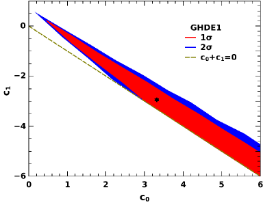
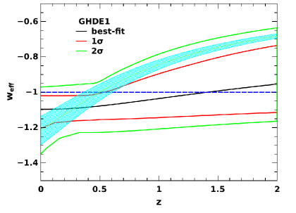
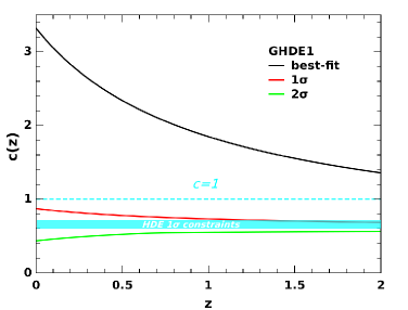
In the left panel of Fig. 1, we plot the 1 and 2 contours for the GHDE1 model in the plane. It is noticeable that the constraints of Eq. (23) (plotted in the black dashed line) is automatically satisfied by the results of the numerical simulation. Another feature of this model is that there is a strong degeneracy between the parameter and . The constrained parameter space distributes roughly along the line .
In the right panel of Fig. 1, we show the evolution of of this model( the of the original HDE model is also showed). Unlike the original HDE model which significant deviates from the CDM model at , here we find that the line lies in roughly the 1 error of the evolution of , with only small deviations in the low redshift region. We also find that the 1 constraints of the CDM and HDE models all lie in the 2 error of the , so they are all consistent with the GHDE1 model in the 2 CL.
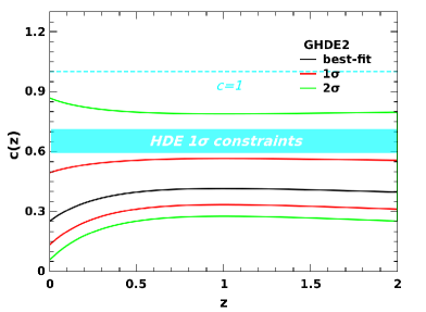
III.2 GHDE2: the JBP type
The “JBP-typ” GHDE model has the following form of :
| (25) |
And it follows directly that,
| (26) |
From Eq. (25), we get: Like the CPL-type parametrization, the JBP parametrization is also unable to describe the behavior of HDE in the future.
In this model, the constraint gives,
| (27) |
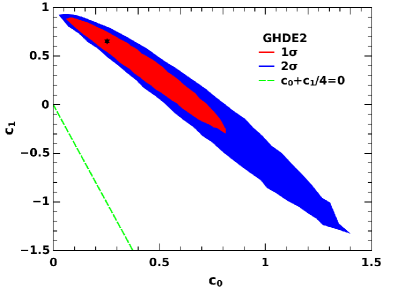
In the left panel of Fig. 2, we plot the 1 and 2 contours for the GHDE2 model in the plane. Again, the requirement of is automatically satisfied. The evolution of of this model is plotted in the right panel of Fig. 2. Like the GHDE1 model, here we also found that both the of the original HDE model and the cosmological constant roughly lie in the 2 error of the evolution of .

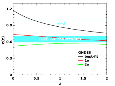
III.3 GHDE3: the Wetterich type
The third parametrization considered is the “Wetterich-type” parametrization, having the following form of ,
| (28) |
It has the property: And it is also straightforward to have
| (29) |
The condition reduces to,
| (30) |
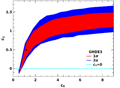
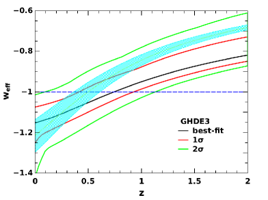
The contours of this model are plotted in the left panel of Fig. 3. Here we find that the requirement of is slightly violated at the small value region of plane. The evolution of of this model is plotted in the right panel of Fig. 3. Unlike the GHDE1 and the GHDE2 model, here we found that both at the very low () and high () redshift regions, the behavior of GHDE deviates from the cosmological constant, while the original HDE model is still consistent with this GHDE model in the 2 CL.
III.4 GHDE4: the Ma-Zhang type
A common short-coming of the above three parametrizations is that they all diverge when the redshift approaches , so we are unable to investigate the future behavior of GHDE in these models. In this section, to overcome this, we consider the following form of , which is proposed in [35]:
| (31) |
It follows directly that
| (32) |
| (33) |
We can find that the of this parametrization is constrained in a finite value even in the future of the universe evolution. Thus this model can have a well-defined property in the far future evolution of the universe, just as the original HDE model which possesses a constant c.
In this model, the requirement of is reduced to,
| (34) |
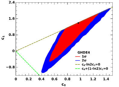
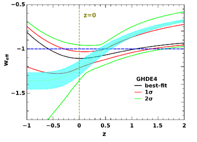
In the left panel of Fig. 4, we plot the 1 and 2 contours for the GHDE4 model in the plane. The constraints of Eq. (34) are automatically satisfied by the numerical simulation results. We also plot the evolution of of this model in the right panel of Fig. 4. A most striking property we find in this model is that the future behavior of could be completely different: while in the original model the behavior of DE is phantom-like in the future, the GHDE in this model can behave like a quintessence, cosmological constant, or phantom. All these possibilities are allowed according to the 2 constraint of the data (see Sec. IV for detailed discussion).
III.5 A Summary of the GHDE Models Considered
In the above subsections, we study four GHDE models with special s. A brief summary of these models are shown in Table 1, where the models, model parameters (together with their best-fit values and 1 uncertainties), and s are given. To make a comparison, the results of the original HDE model and the CDM model (see Ref. [40]) are also listed. Here some nuisance parameters, such as , and mentioned in the appendix, are not shown since they are not model parameters with significant meanings.
From the , we can see that all these models can provide a nice fit to the observational data. Especially, the GHDE2 model showed that the inclusion of the extra parameter can reduce the of the original HDE model by 2.16.
| Model | ||||
|---|---|---|---|---|
| CDM | 424.911 | |||
| HDE | (fixed) | 424.855 | ||
| GHDE1 | 423.369 | |||
| GHDE2 | 422.696 | |||
| GHDE3 | 423.735 | |||
| GHDE4 | 423.407 |
By fitting the observational data, we also get the constraints for those four special forms, which are plotted in Fig. 5. It is found that both the best-fit and the constraint regions of are different among the four GHDE models. As mentioned in Sec. II.2, plays an essential role in characterizing the evolution of DE in the GHDE models. Thus the difference can be interpreted by the different forms of s in these models.
We also find that, although all the ’s best-fits of these four GHDE models distinctly deviate from ’s 1 region of the original HDE model, the 1 constraint of the original HDE model lies well in the 2 region of each GHDE models considered in this work. So we conclude that there are not enough information to determine the form of in the GHDE scenario based on the current cosmological observation data.

IV The Fate of the Universe in the GHDE Scenario
The fate of the universe is always a fascinating issue[41]. In this section, we discuss the fate of the universe in the GHDE scenario. First we study the fate in the original HDE model as a comparison.
IV.1 The fate in the original HDE model
As studied in Sec. II, the behavior of HDE is essentially determined by the parameter . In the original HDE model, the parameter is proposed as a constant, thus the Eq. (18) reduces to,
| (35) |
From the discussion in Sec. II.1, we can find that in the far future, the DE will be the dominated composite of the universe, i.e., . From Eq. (35), we have,
| (36) |
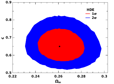
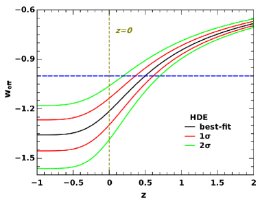
From Eq. (36) the relation between and the fate of the universe can be seen clearly. If , in the far future HDE will behave like a cosmological constant; if , then always we have and HDE behaves as a quintessence; and if , we will have in the future, leading to a phantom universe with big rip as its ultimate fate.
Based on the joint analysis from the SNLS3+BAO+CMB+ data, in the left panel of Fig. 6, the 1 and 2 contours for the HDE model in the plane are plotted. In the 2 CL, we obtain
| (37) |
showing that is significantly favored by the data, which implies that, for the orginal HDE model, there will be in the far future (see the right panel of Fig. 6). Thus, in the orginal HDE model the behavior of HDE is phantom like at last, and the universe will probably end up with a big rip[41].
IV.2 The fate in the GHDE models
In the GHDE scenario, the parameter is not a constant but a function of the redshit . This makes the variety of the HDE behavior increases, and thus let the GHDE model present many more different possibilities for the fate of the universe.
We can focus on the GHDE4 model for a typical demonstration. From Fig. 4, it is interesting to see that various possibilities emerge even in 1 region: the behavior of GHDE in the future evolution can be either quintessence-like or phantom-like, which means the big rip can either happen or not.
Inspired by this fact, one may wonder what forms of can make the HDE processing a purely quintessence-like, phantom-like, or even cosmological-constant-like behavior. This issue is to some extent equivalent with another issue, that is, how to reconstruct a given form of DE component in the GHDE scenario.
For a most general form of DE component, we can describe it by the DE density function ,
| (38) |
Combining with Eqs. (3) and (4), we have
| (39) |
So indeed we can utilizing the GHDE model to reconstruct a DE component with arbitrary from, once given its energy density function .
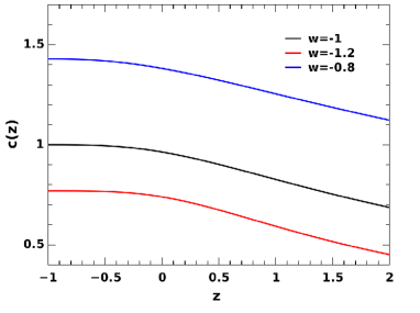
As an example, let us consider the case that the DE component with a constant , i.e. . Neglecting the small , thus
| (40) |
A demonstration is shown in Fig. 7. We take the value and , which correspond to a purely quintessence-like, phantom-like, and cosmological constant behavior, respectively. By numerically integrating the Eq. (40), we get the evolution of for these s. Especially, the case gives the well-known CDM model. Thus, by choosing different forms of s, we can reconstruct a DE component with various behaviors.
As already discussed in the above section, that we can not confirm the form of based on the current cosmological observation data. So, in the GHDE scenario, the fate of the universe remains a mystery.
V Concluding Remarks
In this work, we investigate the generalized holographic dark energy models by considering a redshift-dependent . In all, we consider four parametrizations of , including the CPL type, JBP type, Wetterich type and Ma-Zhang type parametrizations. By performing the joint data analysis, it is shown that all these models can give a nice fit to the data. Among them, the JBP-type GHDE model can even lead to a reduction in the of 2.16.
From the fitting results we also find that the generalization of increase the variety of the HDE model. However, the evolutions of in these models are all consistent with that of the original HDE model in 2 CL. That means, we do not see clear evidence for the evolution of based on the current observational data.
The fate of the universe is always a fascinating issue. Unlike the original HDE model predicting a probably big-rip in the far future, we find that the GHDE model, with the form of undetermined by the current data, lay this issue back to a mystery. Thus for the GHDE model, big-rip or not, it continues to be a question.
At the end, we hope that the method of considering the parameter of the HDE as a redshift-dependent function may provide us some clues to understand the DE problem. In all, more studies about this scenario are needed in the future.
Acknowledgements
We would like to thank Xin Zhang for helpful discussions. This work was supported by the NSFC under Grant Nos. 10535060, 10975172 and 10821504, and by the 973 program (Grant No. 2007CB815401) of the Ministry of Science and Technology of China.
VI Appendix: Observational Data and Methodology
In this work, we adopt the statistic to estimate the model parameters. For a physical quantity with experimentally measured value , standard deviation and theoretically predicted value , the takes the form
| (41) |
The total is the sum of all s, i.e.
| (42) |
One can determine the best-fit model parameters by minimizing the total . Moreover, by calculating , one can determine the 1 and the 2 confidence level (CL) ranges of a specific model. Statistically, for models with different (denoting the number of free model parameters), the 1 and 2 CL correspond to different . In Table 2, we list the relationship between and from to .
In this work, we determine the best-fit parameters and the 1 and 2 CL ranges by using the Monte Carlo Markov chain (MCMC) technique. We modify the publicly available CosmoMC package [42] and generate samples for each set of results presented in this paper. We also verify the reliability and accuracy of the code by using the Mathematica program [43].
| 1 | ||
| 2 | ||
| 3 | ||
| 4 | ||
| 5 | ||
| 6 | ||
| 7 | ||
| 8 | ||
| 9 |
For data, we use the SNLS3 SNIa sample [36], the CMB anisotropy data from the WMAP7 observations [37], the BAO results from the SDSS DR7 [38], and the Hubble constant measurement from the WFC3 on the HST [39]. In the following, we briefly describe how these data are included into the analysis.
VI.1 The SNIa data
Here we use the SNLS3 SNIa dataset released in [36]. This combined sample consists of 472 SN at , including 242 SN over from SNLS 3-yr observations [36], 123 SN at low redshifts [44][45], 93 SN at intermediate redshifts from the SDSS-II SN search [46], and 14 SN at from HST [47]. The systematic uncertainties of the SNIa data were nicely handled [36]. The total data of the SNLS3 sample can be downloaded from [48].
The of the SNIa data is
| (43) |
where C is a covariance matrix capturing the statistic and systematic uncertainties of the SNIa sample, and is a vector of model residuals of the SNIa sample. Here is the rest-frame peak band magnitude of the SNIa, and is the predicted magnitude of the SNIa given by the cosmological model and two other quantities (stretch and color) describing the light-curve of the particular SNIa. The model magnitude is given by
| (44) |
Here is the Hubble-constant free luminosity distance, which takes the form
| (45) |
where and are the CMB frame and heliocentric redshifts of the SN, is the stretch measure for the SN, and is the color measure for the SN. and are nuisance parameters which characterize the stretch-luminosity and color-luminosity relationships, respectively. Following [36], we treat and as free parameters and let them run freely.
The quantity in Eq. (44) is a nuisance parameter representing some combination of the absolute magnitude of a fiducial SNIa and the Hubble constant. In this work, we marginalize following the complicated formula in the Appendix C of [36]. This procedure includes the host-galaxy information [49] in the cosmological fits by splitting the samples into two parts and allowing the absolute magnitude to be different between these two parts.
The total covariance matrix C in Eq. (44) captures both the statistical and systematic uncertainties of the SNIa data. One can decompose it as [36],
| (46) |
where is the purely diagonal part of the statistical uncertainties, is the off-diagonal part of the statistical uncertainties, and is the part capturing the systematic uncertainties. It should be mentioned that, for different and , these covariance matrices are also different. Therefore, in practice one has to reconstruct the covariance matrix for the corresponding values of and , and calculate its inversion. For simplicity, we do not describe these covariance matrices one by one. One can refer to the original paper [36] and the public code [48] for more details about the explicit forms of the covariance matrices and the details of the calculation of .
VI.2 The CMB data
Here we use the “WMAP distance priors” given by the 7-yr WMAP observations [37]. The distance priors include the “acoustic scale” , the “shift parameter” , and the redshift of the decoupling epoch of photons . The acoustic scale , which represents the CMB multipole corresponding to the location of the acoustic peak, is defined as [37]
| (47) |
Here is the proper angular diameter distance, given by
| (48) |
and is the comoving sound horizon size, given by
| (49) |
where and are the present baryon and photon density parameters, respectively. In this paper, we adopt the best-fit values, and (for K), given by the 7-yr WMAP observations [37]. The fitting function of was proposed by Hu and Sugiyama [50]:
| (50) |
where
| (51) |
In addition, the shift parameter is defined as [51]
| (52) |
This parameter has been widely used to constrain various cosmological models [52].
VI.3 The BAO data
Here we use the distance measures from the SDSS DR7 [38]. One effective distance measure is the , which can be obtained from the spherical average [53]
| (55) |
where is the proper angular diameter distance. In this work we use two quantities and . The expression of is given in Eq.(49), and denotes the redshift of the drag epoch, whose fitting formula is proposed by Eisenstein and Hu [54]
| (56) |
where
| (57) | |||||
| (58) |
Following [38], we write the for the BAO data as,
| (59) |
where
| (60) |
and the inverse covariance matrix takes the form
| (61) |
VI.4 The Hubble constant data
The precise measurements of will be helpful to break the degeneracy between it and the DE parameters [55]. When combined with the CMB measurement, it can lead to precise mesure of the DE EOS [56]. Recently, using the WFC3 on the HST, Riess et al. obtained an accurate determination of the Hubble constant [39]
| (62) |
corresponding to a uncertainty. So the of the Hubble constant data is
| (63) |
VI.5 The total
Since the SNIa, CMB, BAO and are effectively independent measurements, we can combine them by simply adding together the functions, i.e.,
| (64) |
References
- [1] A. G. Riess et al., AJ. 116, 1009 (1998); S. Perlmutter et al., ApJ. 517, 565 (1999).
- [2] V. Sahni and A. Starobinsky, IJMP D9, 373 (2000); P. J. E. Peebles and B. Ratra, Rev. Mod. Phys. 75, 559 (2003); T. Padmanabhan, Phys. Rept. 380, 235 (2003); E. J. Copeland, M. Sami and S. Tsujikawa, Int. J. Mod. Phys. D 15, 1753 (2006); A. Albrecht et al., astro-ph/0609591; J. Frieman, M. Turner and D. Huterer, Ann. Rev. Astron. Astrophys 46, 385 (2008); S. Tsujikawa, arXiv:1004.1493; M. Li et al., Commun. Theor. Phys. 56, 525 (2011).
- [3] B. Ratra and P. J. E. Peebles, Phys. Rev. D 37, 3406 (1988); P. J. E. Peebles and B. Ratra, ApJ 325, L17 (1988); C. Wetterich, Nucl. Phys. B302, 668 (1988); I. Zlatev, L. Wang and P. J. Steinhardt, Phys. Rev. Lett. 82, 896 (1999).
- [4] B. Boisseau et al., Phys. Rev. Lett. 85, 2236 (2000); R. R. Caldwell, Phys. Lett. B 545, 23 (2002); S. M. Carroll, M. Hoffman and M. Trodden, Phys. Rev. D 68, 023509 (2003).
- [5] C. Armendariz-Picon, T. Damour and V. Mukhanov, Phys. Lett. B 458, 209 (1999); C. Armendariz-Picon, V. Mukhanov and P. J. Steinhardt, Phys. Rev. D 63, 103510 (2001); T. Chiba, T. Okabe and M. Yamaguchi, Phys. Rev. D 62, 023511 (2000).
- [6] A. Y. Kamenshchik, U. Moschella and V. Pasquier, Phys. Lett. B 511, 265 (2001); M. C. Bento, O. Bertolami and A. A. Sen, Phys. Rev. D 66, 043507 (2002); X. Zhang, F. Q. Wu and J. Zhang, JCAP 0601, 003 (2006); S. Li, Y. G. Ma and Y. Chen, Int. J. Mod. Phys. D 18, 1785 (2009).
- [7] T. Padmanabhan, Phys. Rev. D 66, 021301 (2002); J. S. Bagla, H. K. Jassal, and T. Padmanabhan, Phys. Rev. D 67, 063504 (2003).
- [8] H. Wei, R. G. Cai and D. F. Zeng, Class. Quant. Grav. 22, 3189 (2005); H. Wei and R. G. Cai, Phys. Rev. D 72, 123507 (2005).
- [9] Y. Zhang, T. Y. Xia and W. Zhao, Class. Quant. Grav. 24, 3309 (2007); T. Y. Xia and Y. Zhang, Phys. Lett. B 656, 19 (2007); S. Wang, Y. Zhang and T. Y. Xia, JCAP 10, 037 (2008); S. Wang and Y. Zhang, Phys. Lett. B 669, 201 (2008).
- [10] V. K. Onemli and R. P. Woodard, Class. Quant. Grav. 19, 4607 (2002); V. K. Onemli and R. P. Woodard, Phys. Rev. D 70, 107301 (2004); E. O. Kahya and V. K. Onemli, Phys. Rev. D 76, 043512 (2007); E. O. Kahya, V. K. Onemli and R. P. Woodard, Phys. Rev. D 81, 023508 (2010).
- [11] E. Witten, arXiv:hep-ph/0002297.
- [12] G. ’t Hooft, gr-qc/9310026; L. Susskind, J. Math. Phys. 36, 6377 (1995); J. D. Bekenstein, Phys. Rev. D 7, 2333 (1973); J. D. Bekenstein, Phys. Rev. D 9, 3292 (1974); J. D. Bekenstein, Phys. Rev. D 23, 287 (1981); J. D. Bekenstein, Phys. Rev. D 49, 1912(1994); S. W. Hawking, Commun. Math. Phys. 43, 199 (1975); S. W. Hawking, Phys. Rev. D 13, 191 (1976).
- [13] A. G. Cohen, D. B. Kaplan and A. E. Nelson, Phys. Rev. Lett. 82, 4971 (1999).
- [14] S. D. H. Hsu, Phys. Lett. B 594, 13 (2004).
- [15] M. Li, Phys. Lett. B 603, 1 (2004).
- [16] M. Li, C. S. Lin and Y. Wang, JCAP 0805, 023 (2008).
- [17] M. Li, R. X. Miao and Y. Pang, Phys. Lett. B 689, 55 (2010); M. Li, R. X. Miao and Y. Pang, Opt. Express 18, 9026 (2010).
- [18] C. J. Hogan, astro-ph/0703775; arXiv:0706.1999.
- [19] J. W. Lee, J. Lee and H. C. Kim, JCAP 0708, 005 (2007).
- [20] M. Li and Y. Wang, Phys. Lett. B 687, 243 (2010).
- [21] M. Li et al., Commun. Theor. Phys. 51, 181 (2009).
- [22] M. Li, X. D. Li, S. Wang and X. Zhang, JCAP 0906, 036 (2009).
- [23] H. Wei and R. G. Cai, Phys. Lett. B 655, 1 (2007); R. G. Cai, Phys. Lett. B 657, 228 (2007); H. Wei and R. G. Cai, Phys. Lett. B 660 113 (2008); H. Wei and R. G. Cai, Phys. Lett. B 663, 1 (2008); J. Zhang, X. Zhang and H. Liu, Eur. Phys. J. C 54, 303 (2008); J. P. Wu, D.Z. Ma and Y. Ling, Phys. Lett. B 663, 152 (2008).
- [24] S. Nojiri and S. D. Odintsov, Gen. Rel. Grav. 38, 1285 (2006); C. Gao, F. Wu, X. Chen and Y. G. Shen, Phys. Rev. D 79, 043511 (2009); C. J. Feng, Phys. Lett. B 670, 231 (2008); C. J. Feng, Phys. Lett. B 672, 94 (2009); L. N. Granda and A. Oliveros, Phys. Lett. B 669, 275 (2008); X. Zhang, Phys. Rev. D 79, 103509 (2009); C. J. Feng and X. Zhang, Phys. Lett. B 680, 399 (2009).
- [25] Q. G. Huang and Y. G. Gong, JCAP 0408, 006 (2004); X. Zhang and F. Q. Wu, Phys. Rev. D 72, 043524 (2005); B. Wang, E. Abdalla and R. K. Su, Phys. Lett. B 611, 21 (2005); B. Wang, C. Y. Lin and E. Abdalla, Phys. Lett. B 637, 357 (2006); J. Zhang, X. Zhang and H. Y. Liu, Eur. Phys. J. C 52, 693 (2007); C. J. Feng, Phys. Lett. B 633, 367 (2008); Y. Z. Ma, Y. Gong and X. L. Chen, Eur. Phys. J. C 60, 303 (2009); M. Li et al., JCAP 0912, 014 (2009).
- [26] Q. G. Huang and M. Li, JCAP 0408, 013 (2004).
- [27] Q. G. Huang and M. Li, JCAP 0503, 001 (2005); X. Zhang, Int. J. Mod. Phys. D 14, 1597 (2005); Phys. Lett. B 648, 1 (2007); Phys. Rev. D 74, 103505 (2006); B. Chen, M. Li and Y. Wang, Nucl. Phys. B 774, 256 (2007); J. F. Zhang, X. Zhang and H. Y. Liu, Phys. Lett. B 651, 84 (2007); H. Wei and S. N. Zhang, Phys. Rev. D 76, 063003 (2007); Y. Z. Ma and X. Zhang, Phys. Lett. B 661, 239 (2008); B. Nayak and L. P. Singh, Mod. Phys. Lett. A 24, 1785 (2009); K. Y. Kim, H. W. Lee and Y. S. Myung, Mod. Phys. Lett. A 24, 1267 (2009); Y. G. Gong and T. J. Li, Phys. Lett. B 683, 241 (2010); L. N. Granda, A. Oliveros and W. Cardona, Mod. Phys. Lett. A 25, 1625 (2010); Z. P. Huang and Y. L. Wu, arXiv:1202.4228.
- [28] X. Zhang and F. Q. Wu, Phys. Rev. D 76, 023502 (2007); Z. Chang, F. Q. Wu and X. Zhang, Phys. Lett. B 633, 14 (2006); J. Y. Shen, B. Wang, E. Abdalla and R. K. Su, Phys. Lett. B 609, 200 (2005); Z. L. Yi and T. J. Zhang, Mod. Phys. Lett. A 22, 41 (2007); L. X. Xu et al., Mod. Phys. Lett. A 25, 1441 (2010); Z. P. Huang and Y. L. Wu, arXiv:1202.3517.
- [29] H. M. Sadjadi and M. Honardoost, Phys. Lett. B 647, 231 (2007); K. Y. Kim, H. W. Lee and Y. S. Myung, Mod. Phys. Lett. A 22, 2631 (2007); B. Wang, C. Y. Lin, D. Pavon and E. Abdalla, Phys. Lett. B 662, 1 (2008); J. Zhang, X. Zhang and H. Liu, Phys. Lett. B 659, 26 (2008).
- [30] X. Zhang, Phys. Lett. B 683, 81 (2010).
- [31] H. Wei, Nucl. Phys. B 819, 210 (2009).
- [32] M. Chevallier and D. Polarski, Int. J. Mod. Phys. 10, 213 (2001); E.V. Linder, Phys. Rev. Lett. 90, 091301 (2003).
- [33] H. K. Jassal, J. S. Bagla and T. Padmanabhan, MNRAS. 356, 11 (2005).
- [34] C. Wetterich, Phys. Lett. B 594, 17 (2004); Y. G. Gong, Class. Quantum Grav. 22, 2121(2005).
- [35] J. Z. Ma and X. Zhang, Phys. Lett. B 699, 233 (2011); H. Li and X. Zhang, Phys. Lett. B 703,2 (2011).
- [36] A. Conley et al., ApJS. 192, 1 (2011).
- [37] E. Komatsu et al., ApJS. 192, 18 (2011).
- [38] W. J. Percival et al., MNRAS 401, 2148 (2010).
- [39] A. G. Riess et al., ApJ. 730, 119 (2011).
- [40] X. D. Li et al., JCAP 07, 011 (2011).
- [41] A. A. Starobinsky, Grav. Cosmol. 6, 157 (2000); R. R. Caldwell, M. Kamionkowski and N. N. Weinberg, Phys. Rev. Lett. 91, 071301 (2003).
- [42] A. Lewis and S. Bridle, Phys. Rev. D 66, 103511 (2002).
- [43] http://www.wolfram.com
- [44] M. Hamuy et al., AJ. 112, 2408 (1996); A. G. Riess et al., AJ. 117, 707 (1999); S. Jha et al., AJ. 131, 527 (2006); C. Contreras et al., AJ. 139, 519 (2010).
- [45] M. Hicken, et al., ApJ. 700, 1097 (2009); M. Hicken, et al., ApJ. 700, 331 (2009).
- [46] J. A. Holtzman et al., AJ. 136, 2306 (2008).
- [47] A. G. Riess et al., ApJ. 659, 98 (2007).
- [48] https://tspace.library.utoronto.ca/handle/1807/24512
- [49] M. Sullivan et al., MNRAS 406, 782 (2010).
- [50] W. Hu and N. Sugiyama, ApJ 471, 542 (1996).
- [51] J. R. Bond, G. Efstathiou and M. Tegmark, MNRAS 291, L33 (1997).
- [52] R. Lazkoz, R. Maartens and E. Majerotto, Phys. Rev. D 74, 083510 (2006); O. Elgaroy and T. Multamaki, astro-ph/0702343; M. Li, X. D. Li and S. Wang, arXiv:0910.0717; M. X. Lan, M. Li, X. D. Li and S. Wang, Phys. Rev. D 82, 023516 (2010); S. Wang, X. D. Li, and M. Li, Phys. Rev. D 82, 103006 (2010); H. Wei, JCAP 1008, 020 (2010).
- [53] D. J. Eisenstein et al., ApJ 633, 560 (2005).
- [54] D. J. Eisenstein and W. Hu, ApJ. 496, 605 (1998).
- [55] W. L. Freedman and B. F. Madore, arXiv:1004.1856.
- [56] W. Hu, ASP Conf. Ser. 339, 215 (2005).