Translocation of a polymer chain driven by a dichotomous noise

Abstract

We consider the translocation of a one-dimensional polymer through a pore channel helped by a motor driven by a dichotomous noise with time exponential correlation. We are interested in the study of the translocation time, mean velocity and stall force of the system as a function of the mean driving frequency. We find a monotonous translocation time, in contrast with the mean velocity which shows a pronounced maximum at a given frequency. Interestingly, the stall force shows a nonmonotonic behavior with the presence of a minimum. The influence of the spring elastic constant to the mean translocation times and velocities is also presented.

1 Introduction

Translocation features of polymers through natural and artificial pores is a current active research topic in biophysics and nanotechnology [1, 2, 3]. Motivated by many broad interest experimental results, different models have been introduced to describe and study in a simple way this and related problems. For instance, single barrier potentials [4], as well as flashing ratchet models [5], have been studied to describe the polymer translocation and polymer transport dynamics. The passage of small molecules through passive cell channels can be also modeled by stochastic and rachetlike forces [6]. In some cases the transport phenomena involves not translocation through pores, but also molecular motors, whose complex action has been recently addressed at high attention [7, 8]. In addition, nanotechnological applications try to emulate the complex biological process related to the translocation dynamics [9, 10].

Recently, we have studied different models for the 1d translocation of a spring-bead polymer helped by a motor using a sinusoidal force [11]. The introduction of a time dependent driving force imposes a new time scale on the system, and provides new and richer phenomenology: for sinusoidal driving, the translocation time shows an oscillatory behavior as a function of the frequency.

In order to introduce stochasticity in the motor action and motivated by the relevant role played by dichotomous noise in biological problems, in this manuscript we consider the case of a polymer driven by a two-state force: constant force which pushes the polymer chain in one direction during the activity of the motor, and zero force which leaves the polymer to diffuse freely otherwise. This pure dichotomous mechanism constitutes a first approach in describing a machine working dichotomously between two on-off states [12, 13].

The motor modeled in [12, 13] acts during a fixed time, while the waiting times are exponentially distributed with a mean time depending on the ATP concentration. In the present work a simpler dichotomous mechanism which can well point out, by contrast, the specific behavior of the ATP based machines is studied.

On the other hand, pure dichotomous driving makes sense in the nanotechnological context as well as in the biophysical one. In the first case the passage of a polymer can be induced through a graphene pore or solid state channeling [14, 15] by applying a dichotomous force between the two sides of the layer. In the second case, the model can describe the translocation of a linear molecule through a cell membrane gate having a chemical potential difference between their two sides. The driving is in this case induced by the typical open/close mechanism which follow the purely dichotomous switching largely used in literature [6, 16, 17].

The purpose of our work is to model phenomenologically the possible physical systems described above. We want to stress here the qualitative specific results connected to the purely dichotomous driving.

Thus, differently from the sinusoidal case, no special behavior is observed in the mean translocation time of the polymer for the case here studied. However, for this problem, another observable parameter can be studied. In fact, single molecule experiments are able to detect and use the instantaneous velocity in order to quantify the translocation process in forced systems [7]. Remarkably, we find a non trivial behavior of the polymer translocation velocity as a function of the mean frequency $\nu$ of the driving with the presence of a maximum, even if the translocation time shows only a monotonic behavior. This difference reveals the importance of dealing with several measures to explore the complex behavior of the polymer translocation.

The dependence of the stall force $F_{stall}$ of the machine is also calculated. We find, again, a strong nonmonotonic behavior of $F_{stall}$ with the frequency, similar to the one found in [11].

The paper is organized as follows: first we present the model for polymer and the properties of the stochastic driving force. The main properties of the translocation process are then calculated: translocation time, mean velocity and stall force. Finally, we analyze the dependence of the above properties with the chain stiffness.

2 The model

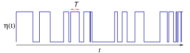
Figure 1: Scheme of a linear chain driven by a dichotomous force restricted to a small space region (width $L_{M}$). $T$ is the mean time during which the force maintains a same value $\{0,F_{M}\}$.

The polymer is modeled as a unidimensional chain of $N$ dimensionless monomers connected by harmonic springs [20].

1d models are suitable in order to describe the dynamics of polymers constrained to move in confined channels [15]. Also, in many experimental situations [7] the polymer is stretched, thus removing the dimensionality dependence of the measured quantities. Moreover, in this work, we want to fix our attention to the motor activity in the translocation more than the delay given by other effects, such as entropic contributions.

The total potential energy is

$$V_{\rm har}=\frac{k}{2}\sum_{i=1}^{N}(x_{i+1}-x_{i}-d_{0})^{2},$$ (1)

where $k$ is the elastic constant, $x_{i}$ the position of the $i$-th particle, and $d_{0}$ the equilibrium distance between adjacent monomers.

The translocation is helped by the presence of a motor which is activated dichotomously. The machine has a spatial working width $L_{M}$ and the position $x=0$ represents the right edge of its action (see Fig. 1). Thus the monomers $i$ such that $x_{i}\in[-L_{M},0]$ experience a force made by the motor. We define $\eta(x,t)$ to represent the dichotomous force, which fluctuates between two values $0$ (no force) and $F_{M}$. Thus

$${\langle\eta(t)\rangle}=\frac{F_{M}}{2}\;\;\,\;{\rm and}\;\;\;{\langle\eta(t)\eta(t^{\prime})\rangle}=\frac{F_{M}^{2}}{4}(1+e^{-2\frac{(t^{\prime}-t)}{T}})$$ (2)

Here $T$ gives the mean residence time in each state. With respect to the spatial dependence

$$\eta(x)=\left\{\begin{array}[]{lr}F_{M}&x\in[-L_{M},0]\vspace{0.2cm}\\ 0&otherwise\end{array}\right.$$ (3)

The dynamics of the $i^{\rm th}$ monomer of the chain is then described by the following overdamped Langevin equations:

$$\dot{x}_{i}=-\frac{\partial{V_{har}}}{\partial{x_{i}}}+\eta(t,x_{i})+\xi_{i}(t)$$ (4)

where the viscosity parameter for each monomer is included in the normalized time units. $\xi_{i}(t)$ stands for Gaussian uncorrelated thermal fluctuation and follows the usual statistical properties $\langle\xi_{i}(t)\rangle=0$ and $\langle\xi_{i}(t)\xi_{j}(t^{\prime})\rangle=2D\delta_{ij}\delta(t^{\prime}-t)$.

3 Results

We performed a set of $N_{exp}=20,000$ numerical experiment with a stochastic Runge-Kutta algorithm, using a time step of $dt=0.01$. The polymer is compound by $N$ monomers and starts with all the spring at the rest length ($d_{0}=1$), and the last monomer of the chain lies at ($x_{N}=0$), just in the final action range of the dichotomous force. The noise intensity is held fixed at the value $D=0.001$, $L_{M}=5.5$, and $N=12$. The choice of the number of monomers $N$, or equivalently the length $L$, is arbitrary and this small number has been used for computational convenience. We note that in a previous work [11], also with 1d chain, it was found that $\tau$ scales with $L^{2}=(N-1)^{2}$. Similarly we find that $v$ scales with $1/N$.

In this first part, the elastic constant $k$ is held equal to 1, a meaningful choice that corresponds to a not too rigid approximation for the polymer. We will study the main observables of the system as a function of the mean frequency transition $\nu=1/T$.

3.1 Translocation times

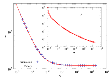
Figure 2: Polymer translocation time $\tau$ as a function of the frequency $\nu$ of the fluctuating force. The solid line shows the theoretical prediction of Eq. 6. In the inset is shown the standard deviation of the exit times distribution.

The translocation time $\tau$ is computed as a mean first passage time of the center of mass of the polymer: the average over the $N_{exp}$ realizations of the time spent by the center of mass of the chain to reach the position $x=0$. In Fig. 2 we see the value of $\tau$ plotted as function of the mean frequency of the driving, and, in the inset, the standard deviation $\sigma$ whose values are of the same order of magnitude than the mean time values, as expected. We find that $\tau$ is a monotonic function of $\nu$. This result is different from that for a periodic force (sinusoidal or square wave ones) where it is observed a minimum in the translocation for $\nu\sim 10^{-2}$ and an oscillating behavior for higher frequencies [11].

In contrast with the behavior of the translocation time, as we will see, the velocity is not a monotonic function of $\nu$ and a maximum is found in this function for $\nu\sim 10^{-2}$ (see Fig. 3). Both effects (minimum translocation time [11] or maximum mean velocity) reveal some interesting similarities with the resonant activation phenomenon [18, 19].

We can make a simple analytical prediction for $\tau(\nu)$ in the low frequency region which however is found to be valid in a broad frequency range (see solid line in Fig. 2). Let $\tau_{on}$ be the value of the exit time when a constant force $F_{M}$ is applied during all the dynamics. In the $\nu\to 0$ limit we have to distinguish between two cases depending on the initial value of the force, $F_{M}$ or $0$. In the first case the translocation time is $\tau_{on}$ corrected in a first approximation by a long waiting time $T$ if the system switches to the off state before $\tau_{on}$, which occurs with a probability $p_{s}=1-e^{\tau_{on}/T}$. This correction gives a contribution of $\tau_{on}(1-p_{s})+(T+\tau_{on})p_{s}$ to the total time. In the second case there is an additional time $T$ in the off state for escaping. Thus the total translocation time is

$$\tau\simeq\frac{1}{2}(\tau_{on}+T(1-e^{\tau_{on}/T}))+\frac{1}{2}(\tau_{on}+T+T(1-e^{\tau_{on}/T}))$$ (5)

Since this equation is derived in the low frequency limit where $1-e^{\tau_{on}/T}\simeq\tau_{on}/T$ we have

$$\tau\simeq 2\tau_{on}+T/2$$ (6)

The intermediate frequency region is characterized by the presence of the constant force alternated by the absence of the force (diffusive dynamics) with an average time ratio between them different for different values of the mean frequency. Surprisingly, Eq. (6) also describes in a good way that frequency region. The third region is instead characterized by a high frequency switching rate between the two force states. There the translocation time is much smaller than $T$, the polymer experiences a mean force $F_{M}/2$, and $\tau\simeq 2\tau_{on}$. A careful observation of our numerical results show that in this high frequency regime

$$\tau\simeq 2\tau_{on}+T,$$ (7)

not observable in Fig.2.

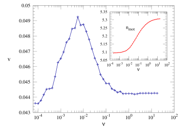
Figure 3: Mean velocity and number of monomers inside the motor while in its active state (inset) as a function of the mean frequency $\nu$ of the fluctuating force.

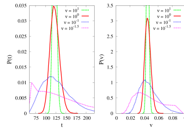
Figure 4: First passage time (left) and velocity (right) probability distributions at four frequency values.

3.2 Mean velocity

Fig. 3 shows the mean velocity $v$ of the polymer as a function of $\nu$. The inset of the figure shows the average number of monomers inside the motor during the active states, $n_{mot}$. We can see that this number is not constant for different values of the mean frequency $\nu$, at least for the value of the elastic constant $k=1$ used in those calculations.

The main result in the velocity curves is the presence of a well pronounced maximum, which put in evidence the qualitative difference between the calculation of the mean first passage time and the mean velocity. In fact, the velocity is computed as $v_{cm}=1/N_{exp}\sum_{i}^{N_{exp}}L/t_{i}$, where $t_{i}$ is the escape time in the $i$-th realization.

As visible in Fig. 4, the exit times distribution changes in shape by changing the mean driving frequency $\nu$. For high values of $\nu$, the time distribution is very narrow around its mean value $\tau$. The corresponding probability distribution function for the velocity is also a narrow function. Decreasing the value of $\nu$, the distributions are more asymmetric and the width increases. The maximum of the time distribution moves toward lower values of time, but the asymmetry changes and higher and higher values of translocation times are involved. That’s why in that region the mean first passage time $\tau$ increases, although the time of the $P(t)$’s maximum decreases. The distribution of the velocity change as well; but because of the increased width of the time distribution, the mean value of the velocity in that region does not follow the relation $v_{med}=1/\tau$ and increases with respect to the high frequency limit, in opposite direction as the one expected from the time behavior. The reason of this effect is that in the average, the smaller times have a higher weight in the inverse $1/t_{i}$ than bigger ones. Thus the mean velocity increases up to a maximum. Decreasing $\nu$ in the low frequency region, the average of the times continues rising up, because the distribution involves higher and higher times. The velocity, however, now decreases since the very high times escapes do not contribute importantly to the mean velocity.

In a first approach the translocation velocity in the high frequency limit is given by

$$v_{l}=\frac{F_{M}}{2}\frac{n_{mot}}{N},$$ (8)

a fraction of monomers given by $n_{mot}/N$ experience a force $F_{M}/2$. Then, the corresponding translocation time is $2\tau_{on}$ (remind that $\tau_{on}$ is the escape time if the motor is always working). On the contrary, in the low frequency limit one half of the realizations give a very long escape time (and velocity goes to zero) and another half give $\tau_{on}$. Thus for low frequencies we obtain the same value of the velocity that for high frequencies.

However, we can see in Fig. 3 that the low frequency limit of the mean velocity does not satisfy the relationship just derived, being lower than the high frequency value $v_{l}$. This happens because the force exerted on the polymer is affected by the number of monomers inside the motor which, as shown in the inset of the figure, also depends on $\nu$. We will see below a confirmation of the given relation by using a strong elastic constant between the monomers, which guarantees a constant number of monomers inside the motor nevertheless the dynamical conditions are (see Fig. 7).

From Eq. (4) it is easy to derive the following equation for the mean velocity

$$v=\frac{1}{N}\frac{1}{N_{exp}}\sum_{i=1}^{N_{exp}}\langle\eta_{i}(t)\rangle_{T}=\frac{F_{M}}{N}\frac{1}{N_{exp}}\sum_{i=1}^{N_{exp}}\frac{n_{\rm mot,i}^{\rm on}(\nu)t^{on}_{i}}{t_{i}},$$ (9)

where, for each experiment $i$, $n_{\rm mot,i}^{\rm on}(\nu)$ is the average number of particles inside the motor when the motor is $on$, $t^{on}_{i}$ is the total motor working time, and $t_{i}$ is the translocation time of each realization.

At high frequency, $t_{i}^{on}=\frac{1}{2}t_{i}$. However, decreasing the frequency for most of the cases, $t_{i}^{on}>\frac{1}{2}t_{i}$, during the translocation the motor spends more time activated that deactivated since most translocations happen during the activation stage of the motor. Thus both, the translocation time and the mean velocity increase. This behavior changes when $1/\nu\sim\tau_{on}$. Then $t_{i}^{on}$ remains constant in Eq. (9), $t_{i}$ increases when $\nu$ decreases and the velocity also decreases towards the expected $v_{l}$ value moderate by the mean number of monomers in the motor in the low frequency limit. This explains the presence of the maximum in the velocity.

A rough estimation of $n_{\rm mot}$ is given by the fixed value $n_{\rm mot}=5.5$, corresponding to the distribution of monomer inside the motor in the case that they maintain the same relative distance, equal to the rest, over all the dynamics. This condition will be completely satisfied for high values of the elastic constant $k$ (rigid chain limit), when $n_{mot}$ becomes independent on $\nu$. As we will see below, both the high and low frequency limits for the mean velocity take in that case the same value (see the inset of Fig. 7)

$$v_{l,theor}=\frac{0.2\cdot 5.5}{2\cdot 12}=0.04583,$$

which is slightly higher than the limit value $v_{l}$ shown in the inset of Fig. 2 because $n_{mot}(k=1)<5.5$.

3.3 Stall Force

The stall force $F_{stall}$ is the force that we need to apply against the motor in order to stop the polymer translocation. It is a measure of the strength of the motor and, in this model, it depends on the frequency of the driving.

Figure 5: A force pull is applied at the first monomer to measure the motor stall force.

A set of simulations have been performed by applying a pull force $F_{p}$ (see Fig. 5) on the left extremum of the chain, in opposite direction to the motor driving force.  The initial condition for the chain has been fixed with the polymer center of mass in the center of the motor. Then, the velocity of the center of mass is measured waiting for the exit on the left or on the right of the motor region. That way, the force for which the mean velocity is zero gives $F_{stall}$.

Fig. 6 shows the stall force as a function of the frequency. As shown in the lower inset, for a given frequency the mean velocity decreases linearly with $F_{p}$. The upper inset, shows that for pull forces of the order of the stall force the velocity presents a minimum, contrary to the behavior at $F_{p}=0$ (Fig. 3). Then the stall force, which presents a similar trend, shows a clear minimum in the same frequency region.

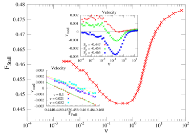
Figure 6: Stall force as a function of the frequency $\nu$ of the driving. The upper inset shows the mean velocity as a function of $\nu$ for the three pull force values $F_{p}=0.447,0.454,0.465$. The bottom  inset shows the linear behavior of the mean velocity as a function of the pull force for the three frequency values $\nu=0.032,0.02,0.1$. The other parameters are the same of Fig. 2.

As in the oscillating case [11], the scale variation of the stall force is small (around $7.5\%$), and an experimental verification of its behavior with the mean frequency the minimum could be not immediately simple to perform.

3.4 Elastic constant dependence

Finally, we investigate the dependence of translocation time and velocity on the elastic constant $k$ of the polymer. A magnitude that strongly depends on $k$ is the mean number of monomer inside the motor during the pushing cycle, $n_{mot}$. This number modules the velocity as it is show in Eq (9). Results are plotted in Fig. 7, where the translocation time and velocity (in the inset) are presented for different value of $k$.

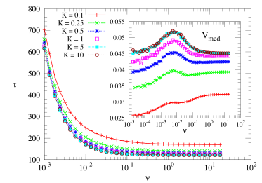
Figure 7: Translocation time and mean velocity (in the inset) of the polymer chain for different values of the elastic constant $k$.

We can see that notable differences (especially visible in the mean velocity plot) are evident by changing the value of $k$. For the case $k=0.1$ the velocity looses the maximum, which is always present for the higher values of $k$. As expected, a clear saturating behavior of the whole curve is evident by increasing $k$ when the chain behaves like a rigid bar. As announced before in the text, in this limit the mean velocity in the cases of both high and low switching frequency gives the expected value $v_{l,theor}$ given above. This limit is already fulfilled for $k=5$.

4 Conclusions

The interest in the introduction of simple models is that they can capture the more relevant features of different processes. In that way, they can result to be very useful for a coarse-grain description of different systems.

The model described here studies the translocation process of a polymer driven by a simple motor which exerts a dichotomous force. We analyze the dependence of the translocation time with the mean frequency of the driving field, and find an analytical expression for the low frequency regime. In spite of the monotonic behavior of the translocation time, the velocity presents a clear maximum at a resonant value of the mean frequency. We argue that this maximum comes from the optimization of the ”on states” duration of the driving forces with the corresponding translocation time. The detection of this maximum, (also seen in the periodic case) could be tackled with the recent single molecule experimental techniques.

The stall force able to stop the polymer translocation against the motor has been also evaluated, finding in our calculations results very close to the oscillating driving, previously studied. The stall force show a very clear minimum at a resonant mean frequency of the driving.

The model can have application in artificial nanotechnological devices driven by dichotomously fluctuating fields, as well as biological pore membrane with intrinsic noise.

This work has been supported by the project FIS2008-01240 of the Spain MICINN.

References

- [1] J. J. Kasianowicz, E. Brandin, D. Branton, and D. W. Deamer, Proc. Natl. Acad. Sci. USA 93, 13770 (1996)
- [2] M.Zwolak and M. Di Ventra, Rev. Mod. Phys 80, 141 (2008)
- [3] G. F. Schneider et al., Nano Lett. 10 3163 (2010).
- [4] N. Pizzolato, A. Fiasconaro, B. Spagnolo, Int. J. Bifurc. Chaos 18, 2871 (2008); N. Pizzolato, A. Fiasconaro, and B. Spagnolo, J. Stat. Mech: Theory and Exp. P01011 (2009).
- [5] M.T. Downton, M.J.Zuckermann, E.M.Craig, M.Plischke, H.Linke, Phys. Rev. E 73, 011909 (2006); E.M.Craig, M.J.Zuckermann, H.Linke, Phys. Rev. E 73, 051106 (2006)
- [6] I. Kosztin and K. Schulten. Phys. Rev. Lett. 93, 238102 (2004)
- [7] D. E. Smith, S. J. Tans, S. B. Smith, S. Grimes, D. L. Anderson, and C. Bustamante, Nature 413, 748 (2001)
- [8] J. R. Moffitt, Y. R. Chemla, K.Aathavan, S. Grimes, P. J. Jardine, D. L. Anderson, and C. Bustamante, Nature 457, 446 (2009).
- [9] M. Mickler, E. Schleiff, and T. Hugel Chem. Phys. Chem. 9, 1503 (2008).
- [10] E. B. Starikov, D. Henning, H. Yamada, R. Gutierrez, B. Norden, and G. Cuniberti, Biophys. Rev. and Lett. 4(3), 209 (2009)
- [11] A. Fiasconaro, F. Falo, and J.J. Mazo, Phys. Rev. E 82, 031803 (2010).
- [12] A. Gomez-Marin and J. M. Sancho, Eur. Phys. Lett. 86, 40002 (2009)
- [13] A. Fiasconaro, F. Falo, and J.J. Mazo. New Journal of Physics 14, 023004 (2012).
- [14] J. Han, S. W. Turner, and H. G. Craighead, Phys. Rev. Lett. 83, 1688 (1999).
- [15] B. Luan, H. Peng, S. Polonsky, S. Rossnagel, G. Stolovitzky, and G. Martyna, Phys. Rev. Lett. 104, 238103 (2010)
- [16] M. M. Millonas,and D. R. Chialvo, Phys. Rev. Lett. 76, 550 (1996).
- [17] A. Kargol and K. Kabza, Physical Biology 5, 026003 (2008).
- [18] N. Pizzolato, A. Fiasconaro, D. Persano Adorno, B. Spagnolo, Physical Biology 7, 034001 (2010).
- [19] C.R. Doering, and J. C. Gadoua, Phys. Rev. Lett. 69, 2318 (1992); M. Bier, and R.D. Astumian, Phys. Rev. Lett. 71, 1649 (1993).
- [20] P. E. J. Rouse, J. Chem. Phys. 21, 1272 (1953).