A Novel MCMC Based Receiver for Large-Scale Uplink
Multiuser MIMO Systems

Abstract

In this paper, we propose low complexity algorithms based on Markov chain Monte Carlo (MCMC) technique for signal detection and channel estimation on the uplink in large scale multiuser multiple input multiple output (MIMO) systems with tens to hundreds of antennas at the base station (BS) and similar number of uplink users. A BS receiver that employs a randomized sampling method (which makes a probabilistic choice between Gibbs sampling and random sampling in each iteration) for detection and a Gibbs sampling based method for channel estimation is proposed. The algorithm proposed for detection alleviates the stalling problem encountered at high SNRs in conventional MCMC algorithm and achieves near-optimal performance in large systems. A novel ingredient in the detection algorithm that is responsible for achieving near-optimal performance at low complexities is the joint use of a randomized MCMC (R-MCMC) strategy coupled with a multiple restart strategy with an efficient restart criterion. Near-optimal detection performance is demonstrated for large number of BS antennas and users (e.g., 64, 128, 256 BS antennas/users). The proposed MCMC based channel estimation algorithm refines an initial estimate of the channel obtained during pilot phase through iterations with R-MCMC detection during data phase. In time division duplex (TDD) systems where channel reciprocity holds, these channel estimates can be used for multiuser MIMO precoding on the downlink. Further, we employ this receiver architecture in the frequency domain for receiving cyclic prefixed single carrier (CPSC) signals on frequency selective fading between users and the BS. The proposed receiver achieves performance that is near optimal and close to that with perfect channel knowledge.

Keywords – Large-scale multiuser MIMO, Markov chain Monte Carlo technique, Gibbs sampling, stalling problem, randomized sampling, multiple restarts, detection, channel estimation, cyclic prefixed single carrier system.

I Introduction

Capacity of multiple-input multiple-output (MIMO) wireless channels is known to increase linearly with the minimum of the number of transmit and receive antennas [1]-[5]. Large-scale MIMO systems with tens to hundreds of antennas have attracted much interest recently [6]-[17]. The motivation to consider such large-scale MIMO systems is the potential to practically realize the theoretically predicted benefits of MIMO, in terms of very high spectral efficiencies/sum rates, increased reliability and power efficiency through the exploitation of large spatial dimensions. Use of large number of antennas is getting recognized to be a good approach to fulfill the increased throughput requirements in future wireless systems. Particularly, large multiuser MIMO wireless systems where the base station (BS) has tens to hundreds of antennas and the users have one or more antennas are widely being investigated [9],[12]-[17]. Communications on the uplink [13],[16] as well as on the downlink [9],[14],[15] in such large systems are of interest. Key issues in large multiuser MIMO systems on the downlink include low complexity precoding strategies and pilot contamination problem encountered in using non-orthogonal pilot sequences for channel estimation in multi-cell scenarios [14]. In large multiuser MIMO systems on the uplink, users with one or more antennas transmit simultaneously to the BS with large number of antennas, and their signals are separated at the BS using the spatial signatures of the users. Sophisticated signal processing is required at the BS receiver to extract the signal of each user from the aggregate received signal [4]. Use of large number of BS antennas has been shown to improve the power efficiency of uplink transmissions in multiuser MIMO using linear receivers at the BS [16]. Linear receivers including matched filter (MF) and minimum mean square error (MMSE) receivers are shown to be attractive for very large number of BS antennas [13]. Our focus in this paper is on achieving near-optimal receiver performance at the BS in large multiuser MIMO systems on the uplink at low complexities. The receiver functions we consider include signal detection and channel estimation. The approach we adopt for both detection as well as channel estimation is Markov chain Monte Carlo (MCMC) approach.

The uplink multiuser MIMO architecture can be viewed as a point-to-point MIMO system with co-located transmit antennas with adequate separation between them (so that there is no or negligible spatial correlation among them), and no cooperation among these transmit antennas [4]. Because of this, receiver algorithms for point-to-point MIMO systems are applicable for receiving uplink multiuser MIMO signals at the BS receiver. Recently, there has been encouraging progress in the development of low-complexity near-optimal MIMO receiver algorithms that can scale well for large dimensions [8],[10],[18]-[25]. These algorithms are based on techniques from local neighborhood search including tabu search [8],[10],[18]-[21], probabilistic data association [22], and message passing on graphical models including factor graphs and Markov random fields [23],[24],[25].

Another interesting class of low-complexity algorithms reported in the context of CDMA and MIMO detection is based on Markov chain Monte Carlo (MCMC) simulation techniques [26]-[33]. MCMC techniques are computational techniques that make use of random numbers [34]. MCMC methods have their roots in the Metropolis algorithm, an attempt by physicists to compute complex integrals by expressing them as expectations for some distribution and then estimating this expectation by drawing samples from that distribution [35],[36]. In MCMC methods, statistical inferences are developed by simulating the underlying processes through Markov chains. By doing so, it becomes possible to reduce exponential detection complexity to linear/polynomial complexities. An issue with conventional MCMC based detection, however, is the stalling problem, due to which performance degrades at high SNRs [27]. Stalling problem arises because transitions from some states to other states in a Markov chain can occur with very low probability [27]. Our first contribution in this paper is that we propose an MCMC based detection algorithm that alleviates the stalling problem encountered in conventional MCMC and achieves near-optimal performance in large systems. A key idea that is instrumental in alleviating the stalling problem is a randomized sampling strategy that makes a probabilistic choice between Gibbs sampling and random sampling in each iteration. An efficient stopping criterion aids complexity reduction. This randomized sampling strategy, referred to as randomized MCMC (R-MCMC) strategy, is shown to achieve near-optimal performance in multiuser MIMO systems with 16 to 256 BS antennas and same number of uplink users for 4-QAM [37]. However, we find that this randomized sampling strategy alone is not adequate to achieve near-optimal performance at low complexities for higher-order QAM (e.g., 16-QAM, 64-QAM). We show that near-optimal performance is achieved in higher-order QAM also if a multiple restart strategy is performed in conjunction with R-MCMC. We refer to this strategy as ‘R-MCMC with restarts’ (R-MCMC-R) strategy. Here again, an efficient restart criterion aids complexity reduction. The joint use of both randomized sampling as well as multiple restart strategies is found to be crucial in achieving near-optimal performance for higher-order QAM in large systems. To our knowledge, the closeness to optimal performance achieved by the proposed R-MCMC-R algorithm for tens to hundreds of BS antennas/users with higher-order QAM has not been reported so far using other MCMC based algorithms in the literature.

Channel estimation at the BS is an important issue in large multiuser MIMO systems on the uplink. While channel estimation at the BS is needed for uplink signal detection, in TDD systems where channel reciprocity holds, the estimated channel can also be used for precoding purposes on the downlink avoiding the need for feeding back channel estimates from the users. Our second contribution in this paper is that we propose an MCMC based uplink channel estimation algorithm at the BS receiver. The algorithm employs Gibbs sampling to refine an initial estimate of the channel obtained during the pilot phase, through iterations with R-MCMC-R detection during the data phase. The algorithm is shown to yield good mean square error (MSE) and bit error rate (BER) performance in large multiuser MIMO systems (e.g., 128 BS antennas/users). BER Performance close to that with perfect channel knowledge is achieved. Finally, we employ the proposed MCMC based algorithms for equalization and channel estimation in frequency selective fading between the users and BS. Because of $i)$ their advantage of avoiding the peak-to-average power ratio (PAPR) problem that is encountered in multicarrier systems and $ii)$ their good performance, cyclic prefixed single carrier (CPSC) transmissions [39]-[41] from the uplink users are considered. The proposed MCMC algorithms are shown to work well in receiving uplink CPSC transmissions in frequency selective fading as well.

The rest of the paper is organized as follows. The uplink multiuser MIMO system model on frequency non-selective fading is presented in Section II. The proposed R-MCMC algorithm without and with multiple restarts and its performance/complexity results in frequency non-selective fading are presented in Section III. Section IV presents the proposed MCMC based channel estimation algorithm and its performance. Section V presents the proposed receiver for frequency domain equalization of CPSC signals and channel estimation in frequency selective fading. Conclusions are presented in Section VI.

II System Model

Consider a large-scale multiuser MIMO system on the uplink consisting of a BS with $N$ receive antennas and $K$ homogeneous uplink users with one transmit antenna each, $K\leq N$ (Fig. 1). Extension to system model with non-homogeneous users where different users can have different number of transmit antennas is straightforward. $N$ and $K$ are in the range of tens to hundreds. All users transmit symbols from a modulation alphabet $\mathbb{B}$. It is assumed that synchronization and sampling procedures have been carried out, and that the sampled base band signals are available at the BS receiver. Let $x_{k}\in\mathbb{B}$ denote the transmitted symbol from user $k$. Let ${\bf x}_{c}=[x_{1},x_{2},\cdots,x_{K}]^{T}$ denote the vector comprising of the symbols transmitted simultaneously by all users in one channel use. Let ${\bf H}_{c}\in\mathbb{C}^{N\times K}$, given by ${\bf H}_{c}=[{\bf h}_{1},{\bf h}_{2},\cdots,{\bf h}_{K}]$, denote the channel gain matrix, where ${\bf h}_{k}=[h_{1k},h_{2k},\cdots,h_{Nk}]^{T}$ is the channel gain vector from user $k$ to BS, and $h_{jk}$ denotes the channel gain from $k$th user to $j$th receive antenna at the BS. Assuming rich scattering and adequate spatial separation between users and BS antenna elements, $h_{jk},\forall j$ are assumed to be independent Gaussian with zero mean and $\sigma_{k}^{2}$ variance such that $\sum_{k}\sigma_{k}^{2}=K$. $\sigma_{k}^{2}$ models the imbalance in received powers from different users, and $\sigma_{k}^{2}=1$ corresponds to the perfect power control scenario. This channel gain model amounts to assuming that the multipath fading between a user and BS is frequency non-selective. Frequency selective fading is considered in Section V. Now, the received signal vector at the BS in a channel use, denoted by ${\bf y}_{c}\in\mathbb{C}^{N}$, can be written as

$${\bf y}_{c} = {\bf H}_{c}{\bf x}_{c}+{\bf n}_{c},$$ (1)

where ${\bf n}_{c}$ is the noise vector whose entries are are modeled as i.i.d. ${\mathbb{C}}{\mathcal{N}}(0,\sigma^{2})$. We will work with the real-valued system model corresponding to (1), given by

$${\bf y}_{r} = {\bf H}_{r}\,{\bf x}_{r}+{\bf n}_{r},$$ (2)

where ${\bf x}_{r}\in\mathbb{R}^{2K}$, ${\bf H}_{r}\in\mathbb{R}^{2N\times 2K}$, ${\bf y}_{r}\in\mathbb{R}^{2N}$, ${\bf n}_{r}\in\mathbb{R}^{2N}$ given by

$${\bf H}_{r}=\left[\begin{array}[]{cc}\Re({\bf H}_{c})\hskip 5.69054pt-\Im({\bf H}_{c})\\ \Im({\bf H}_{c})\hskip 14.22636pt\Re({\bf H}_{c})\end{array}\right],\quad{\bf y}_{r}=\left[\begin{array}[]{c}\Re({\bf y}_{c})\\ \Im({\bf y}_{c})\end{array}\right],\quad{\bf x}_{r}=\left[\begin{array}[]{c}\Re({\bf x}_{c})\\ \Im({\bf x}_{c})\end{array}\right],\quad{\bf n}_{r}=\left[\begin{array}[]{c}\Re({\bf n}_{c})\\ \Im({\bf n}_{c})\end{array}\right].$$

Dropping the subscript $r$ in (2) for notational simplicity, the real-valued system model is written as

$${\bf y} = {\bf H}{\bf x}+{\bf n}.$$ (3)

For a QAM alphabet ${\mathbb{B}}$, the elements of ${\bf x}$ will take values from the underlying PAM alphabet ${\mathbb{A}}$, i.e., ${\bf x}\in\mathbb{A}^{2K}$. The symbols from all the users are jointly detected at the BS. The maximum likelihood (ML) decision rule is given by

$${\bf x}_{ML} = {\arg\min_{{\bf x}\in{\mathbb{A}}^{2K}}}\|{\bf y}-{\bf H}{\bf x}\|^{2}\,\,=\,\,{\arg\min_{{\bf x}\in{\mathbb{A}}^{2K}}}\,f({\bf x}),$$ (4)

where $f({\bf x})\stackrel{{\scriptstyle\triangle}}{{=}}{\bf x}^{T}{\bf H}^{T}{\bf H}{\bf x}-2{\bf y}^{T}{\bf H}{\bf x}$ is the ML cost. While the ML detector in (4) is exponentially complex in $K$ (which is prohibitive for large $K$), the MCMC based algorithms we propose in the next section have quadratic complexity in $K$ and they achieve near-ML performance as well.

III Proposed Randomized-MCMC Algorithm for Detection

The ML detection problem in (4) can be solved by using MCMC simulations [34]. We consider Gibbs sampler, which is an MCMC method used for sampling from distributions of multiple dimensions. In the context of MIMO detection, the joint probability distribution of interest is given by

$$p(x_{1},\cdots,x_{2K}|\bf{y},\bf{H}) \propto \exp\Big{(}-\frac{\parallel\bf{y}-\bf{H}\bf{x}\parallel^{2}}{\sigma^{2}}\Big{)}.$$ (5)

We assume frequency non-selective fading and perfect knowledge of channel gain matrix ${\bf H}$ at the BS receiver in this section. We will relax the perfect channel knowledge assumption by proposing a MCMC based channel estimation algorithm in section IV.

III-A Conventional MCMC algorithm

In conventional Gibbs sampling based detection, referred to as conventional MCMC algorithm, the algorithm starts with an initial symbol vector, denoted by ${\bf x}^{(t=0)}$. In each iteration of the algorithm, an updated symbol vector is obtained by sampling from distributions as follows:

$${x}^{(t+1)}_{1} \thicksim p(x_{1}|x^{(t)}_{2},{x}^{(t)}_{3},\cdots,x^{(t)}_{2K}),$$

$$x^{(t+1)}_{2} \thicksim p(x_{2}|x^{(t+1)}_{1},x^{(t)}_{3},\cdots,x^{(t)}_{2K}),$$

$$x^{(t+1)}_{3} \thicksim p(x_{3}|x^{(t+1)}_{1},x^{(t+1)}_{2},x^{(t)}_{4},\cdots,x^{(t)}_{2K}),$$

$$\vdots$$

$$x^{(t+1)}_{2K} \thicksim p(x_{2K}|x^{(t+1)}_{1},x^{(t+1)}_{2},\cdots,x^{(t+1)}_{2K-1}).$$ (6)

The detected symbol vector in a given iteration is chosen to be that symbol vector which has the least ML cost in all the iterations up to that iteration. Another MCMC algorithm that uses a temperature parameter $\alpha$ and the following joint distribution is presented in [33]:

$$p(x_{1},\cdots,x_{2K}|\bf{y},\bf{H}) \propto \exp\Big{(}-\frac{\parallel\bf{y}-\bf{H}\bf{x}\parallel^{2}}{\alpha^{2}\sigma^{2}}\Big{)}.$$ (7)

The algorithm uses a fixed value of $\alpha$ in all the iterations, with the property that after the Markov chain is mixed, the probability of encountering the optimal solution is only polynomially small (not exponentially small). This algorithm and the conventional MCMC algorithm (which is a special case of $\alpha=1$) face stalling problem at high SNRs; a problem in which the BER performance gets worse at high SNRs [27].

III-B Proposed R-MCMC algorithm

It is noted that the stalling problem occurs due to MCMC iterations getting trapped in poor local solutions, beyond which the ML cost does not improve with increasing iterations for a long time. Motivated by this observation, we propose a simple, yet effective, randomization strategy to avoid such traps. The key idea behind the proposed randomized MCMC (R-MCMC) approach is that, in each iteration, instead of updating $x_{i}^{(t)}$’s as per the update rule in (6) with probability 1 as in conventional MCMC, we update them as per (6) with probability $(1-q_{i})$ and use a different update rule with probability $q_{i}=\frac{1}{2K}$. The different update rule is as follows. Generate $|{\mathbb{A}}|$ probability values from uniform distribution as

$$p(x_{i}^{(t)}=j)\thicksim U[0,1],\quad\forall j\in{\mathbb{A}}$$

such that $\sum\limits_{j=1}^{|{\mathbb{A}}|}p(x_{i}^{(t)}=j)=1$, and sample $x_{i}^{(t)}$ from this generated pmf.

III-B1 Proposed stopping criterion

A suitable termination criterion is needed to stop the algorithm. A simple strategy is to terminate the algorithm after a fixed number of iterations. But a fixed value of number of iterations may not be appropriate for all scenarios. Fixing a large value for the number of iterations can yield good performance, but the complexity increases with the number of iterations. To address this issue, we develop a dynamic stopping criterion that yields good performance without unduly increasing the complexity. The criterion works as follows. A stalling is said to have occurred if the ML cost remains unchanged in two consecutive iterations. Once such a stalling is identified, the algorithm generates a positive integer $\Theta_{s}$ (referred to as the stalling limit), and the iterations are allowed to continue in stalling mode (i.e., without ML cost change) up to a maximum of $\Theta_{s}$ iterations from the occurrence of stalling. If a lower ML cost is encountered before $\Theta_{s}$ iterations, the algorithm proceeds with the newly found lower ML cost; else, the algorithm terminates. If termination does not happen through stalling limit as above, the algorithm terminates on completing a maximum number of iterations, MAX-ITER.

The algorithm chooses the value of $\Theta_{s}$ depending on the quality of the stalled ML cost, as follows. A large value for $\Theta_{s}$ is preferred if the quality of the stalled ML cost is poor, because of the available potential for improvement from a poor stalled solution. On the other hand, if the stalled ML cost quality is already good, then a small value of $\Theta_{s}$ is preferred. The quality of a stalled solution is determined in terms of closeness of the stalled ML cost to a value obtained using the statistics (mean and variance) of the ML cost for the case when ${\bf x}$ is detected error-free. Note that when ${\bf x}$ is detected error-free, the corresponding ML cost is nothing but $\|{\bf n}\|^{2}$, which is Chi-squared distributed with $2N$ degrees of freedom with mean $N\sigma^{2}$ and variance $N\sigma^{4}$. We define the quality metric to be the difference between the ML cost of the stalled solution and the mean of $\|{\bf n}\|^{2}$, scaled by the standard deviation, i.e., the quality metric of vector $\hat{\bf x}$ is defined as

$$\phi({\hat{\bf x}})=\frac{\|{\bf y}-{\bf H}\hat{{\bf x}}\|^{2}-N\sigma^{2}}{\sqrt{N}\sigma^{2}}.$$ (8)

We refer to the metric in (8) as the standardized ML cost of solution vector $\hat{\bf x}$. A large value of $\phi(\hat{\bf x})$ can be viewed as an indicator of increased closeness of $\hat{\bf x}$ to ML solution. Therefore, from the previous discussion, it is desired to choose the stalling limit $\Theta_{s}$ to be an increasing function of $\phi({\hat{\bf x}})$. For this purpose, we choose an exponential function of the form

$$\Theta_{s}(\phi(\hat{{\bf x}}))=c_{1}\exp(\phi(\hat{{\bf x}})).$$ (9)

Also, we allow a minimum number of iterations ($c_{min}$) following a stalling. Based on the above discussion, we adopt the following rule to compute the stalling count:

$$\Theta_{s}(\hat{\bf x})=\left\lceil\max\left(c_{min},c_{1}\exp\left(\phi(\hat{{\bf x}})\right)\right)\right\rceil.$$ (10)

The constant $c_{1}$ is chosen depending upon the QAM size; a larger $c_{1}$ is chosen for larger QAM size. As we will see in the performance and complexity results, the proposed randomization in the update rule and the stopping criterion are quite effective in achieving low complexity as well as near-optimal performance. A complete listing of the proposed R-MCMC algorithm incorporating the randomized sampling and stopping criterion ideas is given in the next page.

Algorithm 1 Proposed randomized-MCMC algorithm

1:  input: ${\bf y}$, ${\bf H}$, ${\bf x}^{(0)};$ ${\bf{x}}^{(0)}:$ initial vector $\in{\mathbb{A}}^{2K}$;    MAX-ITER: max. # iterations;

2:  $t=0$;    ${\bf z}={\bf x}^{(0)}$;    $S=\{1,2,\cdots,2K\}$;    $S:$ index set;

3:  $\beta=f({\bf{x}}^{(0)});\quad f(.):$ ML cost function;    $\Theta_{s}(.):$ stalling limit function;

4:  while $t<$ MAX-ITER do

5:     for $i=1$ to $2K$ do

6:        randomly choose an index $k$ from the set $S$;

7:        if $(i\neq k)$ then

8:           ${x}^{(t+1)}_{i}\thicksim p(x_{i}|{x}^{(t+1)}_{1},\cdots,{x}^{(t+1)}_{i-1},{x}^{(t)}_{i+1},\cdots,{x}^{(t)}_{2K})$

9:        else

10:           generate pmf $p(x_{i}^{(t+1)}=j)\thicksim U[0,1],\,\,\forall j\in{\mathbb{A}}$

11:           sample $x_{i}^{(t)}$ from this pmf

12:        end if

13:     end for

14:     $\gamma=f({\bf{x}}^{(t+1)});$

15:     if $(\gamma\leq\beta)$ then

16:        ${\bf z}={\bf x}^{(t+1)};$     $\beta=\gamma$;

17:     end if

18:     $t=t+1;$

19:     $\beta_{v}^{(t)}=\beta;$

20:     if $\beta_{v}^{(t)}==\beta_{v}^{(t-1)}$ then

21:        calculate $\Theta_{s}({\bf z})$;

22:        if $\Theta_{s}<t$ then

23:           if $\beta_{v}^{(t)}==\beta_{v}^{\left(t-\Theta_{s}\right)}$ then

24:              goto step 29

25:           end if

26:        end if

27:     end if

28:  end while

29:  output: ${\bf z}.\qquad{\bf z}:$ output solution vector

III-B2 Performance and complexity of the R-MCMC algorithm

The simulated BER performance and complexity of the proposed R-MCMC algorithm in uplink multiuser MIMO systems with 4-QAM are shown in Figs. 2 to 6. The following R-MCMC parameters are used in the simulations: $c_{min}=10$, $c_{1}=20$, MAX-ITER $=16K$. Figures 2 to 5 are for the case where there is no imbalance in the received powers of all users, i.e., $\sigma_{k}^{2}=0$ dB $\forall\,k$. Perfect channel knowledge at the BS is assumed. The performance of R-MCMC in multiuser MIMO with $K=N=16$ is shown in Fig. 2. The performance of the MCMC algorithm using the distribution in (7) with temperature parameter values $\alpha=1,1.5,2,3$ are also plotted. $16K$ iterations are used in the MCMC algorithm with temperature parameter. Sphere decoder performance is also shown for comparison. It is seen that the performance of MCMC with temperature parameter is very sensitive to the choice of the value of $\alpha$. For example, for $\alpha=1,1.5$, the BER is found to degrade at high SNRs due to stalling problem. For $\alpha=2$, the performance is better at high SNRs but worse at low SNRs. The proposed R-MCMC performs better than MCMC with temperature parameter (or almost the same) at all SNRs and $\alpha$ values shown. In fact, the performance of R-MCMC is almost the same as the sphere decoder performance. The R-MCMC complexity is, however, significantly lower than the sphere decoding complexity. While sphere decoder gets exponentially complex in $K$ at low SNRs, the R-MCMC complexity (in average number of real operations per bit) is only $O(K^{2})$ as can be seen in Fig. 3. Because of this low complexity, the R-MCMC algorithm scales well for large-scale systems with large values of $K$ and $N$. This is illustrated in Fig. 4 and 5 where performance plots for systems up to $K=N=128$ and 256 are shown. While Fig. 4 shows the BER as a function of SNR, Fig. 5 shows the average received SNR required to achieve a target BER of $10^{-3}$ as a function of $K=N$. Since sphere decoder complexity is prohibitive for hundreds of dimensions, we have plotted unfaded single-input single-output (SISO) AWGN performance as a lower bound on ML performance for comparison. It can be seen that R-MCMC achieves performance which is very close to SISO AWGN performance for large $K=N$, e.g., close to within 0.5 dB at $10^{-3}$ BER for $K=N=128$ and 256. This illustrates the achievability of near-optimal performance using R-MCMC for large systems. Figure 6 shows the BER performance in multiuser MIMO systems with received power imbalance among different users. The imbalance is simulated by choosing different $\sigma_{k}^{2}$ for different users, with $\sigma_{k}^{2}$ being uniformly distributed between -3 dB to 3 dB. Performance in systems with $K=N=16$ and 128 are plotted with and without power imbalance. It is seen that even with power imbalance R-MCMC achieves almost the same performance as that of sphere decoder for $K=N=16$.

III-C Multi-restart R-MCMC algorithm for higher-order QAM

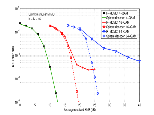
Although the R-MCMC algorithm is very attractive in terms of both performance as well as complexity for 4-QAM, its performance for higher-order QAM is far from optimal. This is illustrated in Fig. 7, where R-MCMC is seen to achieve sphere decoder performance for 4-QAM, whereas for 16-QAM and 64-QAM it performs poorly compared to sphere decoder. This observation motivates the need for ways to improve R-MCMC performance in higher-order QAM. Interestingly, we found that use of multiple restarts coupled with R-MCMC is able to significantly improve performance and achieve near-ML performance in large systems with higher-order QAM.

III-C1 Effect of restarts in R-MCMC and conventional MCMC

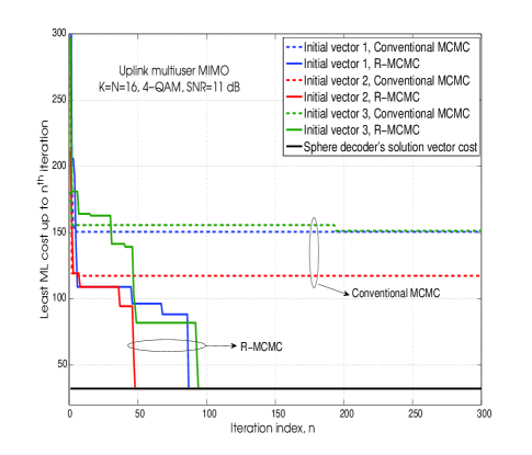
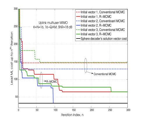
In Figs. 8(a) and 8(b), we compare the effect of multiple random restarts in R-MCMC and conventional MCMC algorithms for 4-QAM and 16-QAM, respectively. For a given realization of ${\bf x},{\bf H}$ and ${\bf n}$, we ran both algorithms for three different random initial vectors, and plotted the least ML cost up to $n$th iteration as a function of $n$. We show the results of this experiment for multiuser MIMO with $K=N=16$ at 11 dB SNR for 4-QAM and 18 dB SNR for 16-QAM (these SNRs give about $10^{-3}$ BER with sphere decoding for 4-QAM and 16-QAM, respectively). The true ML vector cost (obtained through sphere decoder simulation for the same realization) is also plotted. It is seen that R-MCMC achieves much better least ML cost compared to conventional MCMC. This is because conventional MCMC gets locked up in some state (with very low state transition probability) for long time without any change in ML cost in subsequent iterations, whereas the randomized sampling strategy in R-MCMC is able to exit from such states quickly and give improved ML costs in subsequent iterations. This shows that R-MCMC is preferred over conventional MCMC. Even more interestingly, comparing the least ML costs of 4-QAM and 16-QAM (in Figs. 8(a) and (b), respectively), we see that all the three random initializations could converge to almost true ML vector cost for 4-QAM within 100 iterations, whereas only initial vector 3 converges to near true ML cost for 16-QAM and initial vectors 1 and 2 do not. Since any random initialization works well with 4-QAM, R-MCMC is able to achieve near-ML performance without multiple restarts for 4-QAM. However, it is seen that 16-QAM performance is more sensitive to the initialization, which explains the poor performance of R-MCMC without restarts in higher-order QAM. MMSE vector can be used as an initial vector, but it is not a good initialization for all channel realizations. This points to the possibility of achieving good initializations through multiple restarts to improve the performance of R-MCMC in higher-order QAM.

III-C2 R-MCMC with multiple restarts

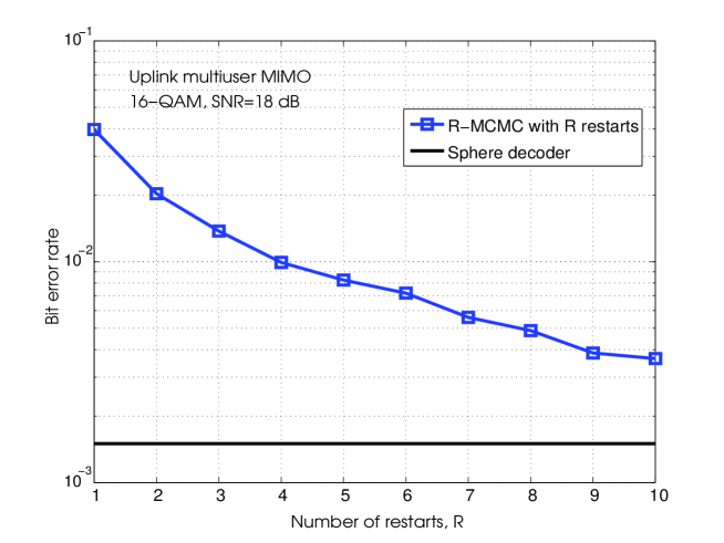
In R-MCMC with multiple restarts, we run the basic R-MCMC algorithm multiple times, each time with a different random initial vector, and choose that vector with the least ML cost at the end as the solution vector. Figure 9 shows the improvement in the BER performance of R-MCMC as the number of restarts ($R$) is increased in multiuser MIMO with $K=N=16$ and 16-QAM at SNR = 18 dB. 300 iterations are used in each restart. It can be observed that, though BER improves with increasing $R$, much gap still remains between sphere decoder performance and R-MCMC performance even with $R=10$. A larger $R$ could get the R-MCMC performance close to sphere decoder performance, but at the cost of increased complexity. While a small $R$ results in poor performance, a large $R$ results in high complexity. So, instead of arbitrarily fixing $R$, there is a need for a good restart criterion that can significantly enhance the performance without incurring much increase in complexity. We devise one such criterion below.

III-C3 Proposed restart criterion

At the end of each restart, we need to decide whether to terminate the algorithm or to go for another restart. To do that, we propose to use

• the standardized ML costs (given by (8)) of solution vectors, and

• the number of repetitions of the solution vectors.

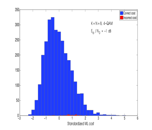
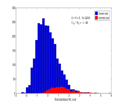
Nearness of the ML costs obtained so far to the error-free ML cost in terms of its statistics can allow the algorithm to get near ML solution. Checking for repetitions can allow restricting the number of restarts, and hence the complexity. In particular, we define multiple thresholds that divide the range of the distribution of $\|{\bf n}\|^{2}$ (i.e., $\mathbb{R}^{+}$) into multiple regions, and define one integer threshold for each of these regions for the purpose of comparison with number of repetitions. We use the minimum standardized ML cost obtained so far and its number of repetitions to decide the credibility of the solution. In Fig 10, we plot histograms of the standardized ML cost of correct and incorrect solution vectors at the output of R-MCMC with restarts in multiuser MIMO with $K=N=8$ and 4-/16-QAM. We judge the correctness of the obtained solution vector from R-MCMC output by running sphere decoder simulation for the same realizations. It can be observed in Fig. 10 that the incorrect standardized ML cost density does not stretch into negative values. Hence, if the obtained solution vector has negative standardized ML cost, then it can indeed be correct with high probability. But as the standardized ML cost increases in the positive domain, the reliability of that vector decreases and hence it would require more number of repetitions for it to be trusted as the final solution vector. It can also be observed from Fig. 10 that the incorrect density in case of 16-QAM is much more than that of 4-QAM for the same SNR. So it is desired that, for a standardized ML cost in the positive domain, the number of repetitions needed to declare as the final solution should increase with the QAM size. Accordingly, the number of repetitions needed for termination ($P$) is chosen as per the following expression:

$$P=\left\lfloor\max\left(0,c_{2}\phi(\tilde{{\bf x}})\right)\right\rfloor+1,$$ (11)

where $\tilde{{\bf x}}$ is the solution vector with minimum ML cost so far. Now, denoting $R_{max}$ to be the maximum number for restarts, the proposed R-MCMC with restarts algorithm (we refer to this as the R-MCMC-R algorithm) can be stated as follows.

• Step 1: Choose an initial vector.

• Step 2: Run the basic R-MCMC algorithm in Sec. III-B.

• Step 3: Check if $R_{max}$ number of restarts have been completed. If yes, go to Step 5; else go to Step 4.

• Step 4: For the solution vector with minimum ML cost obtained so far, find the required number of repetitions needed using (11). Check if the number of repetitions of this solution vector so far is less than the required number of repetitions computed in Step 4. If yes, go to Step 1, else go to Step 5.

• Step 5: Output the solution vector with the minimum ML cost so far as the final solution.

III-C4 Performance and complexity of the R-MCMC-R Algorithm

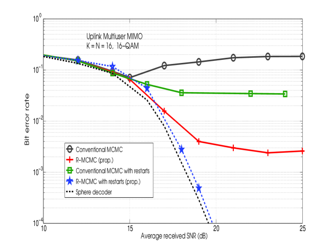
The BER performance and complexity of the R-MCMC-R algorithm are evaluated through simulations. The following parameters are used in the simulations of R-MCMC and R-MCMC-R: $c_{min}=10$, $c_{1}=10\log_{2}M$ (i.e., $c_{2}=20,40,60$ for 4-/16-/64-QAM, respectively), MAX-ITER = $8K\sqrt{M}$, $R_{max}=50$, and $c_{2}=0.5\log_{2}M$. In Fig. 11, we compare the BER performance of conventional MCMC, R-MCMC, R-MCMC-R and sphere decoder in multiuser MIMO with $K=N=16$ and 16-QAM. In the first restart, MMSE solution vector is used as the initial vector. In the subsequent restarts, random initial vectors are used. For 64-QAM, the randomized sampling is applied only to the one-symbol away neighbors of the previous iteration index; this helps to reduce complexity in 64-QAM. From Fig. 11, it is seen that the performance of conventional MCMC, either without or with restarts, is quite poor. That is, using restarts in conventional MCMC is not of much help. This shows the persistence of the stalling problem. The performance of R-MCMC (without restarts) is better than conventional MCMC with and without restarts, but its performance still is far from sphere decoder performance. This shows that R-MCMC alone (without restarts) is inadequate the alleviate the stalling problem in higher-order QAM. However, the randomized sampling in R-MCMC when used along with restarts (i.e., R-MCMC-R) gives strikingly improved performance. In fact, the proposed R-MCMC-R algorithm achieves almost sphere decoder performance (close to within 0.4 dB at $10^{-3}$ BER). This points to the important observations that application of any one of the two features, namely, randomized sampling and restarts, to the conventional MCMC algorithm is not adequate, and that simultaneous application of both these features is needed to alleviate the stalling problem and achieve near-ML performance in higher-order QAM.

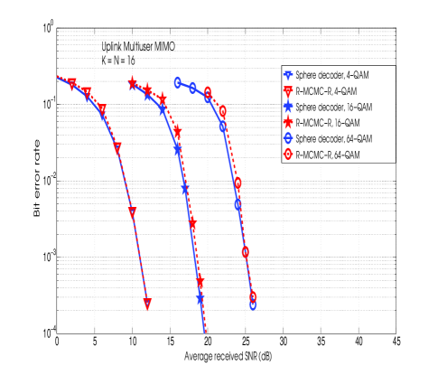
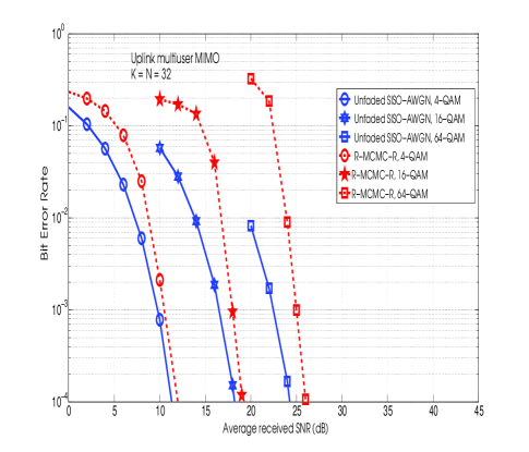
Figure 12(a) shows that the R-MCMC-R algorithm is able to achieve almost sphere decoder performance for 4-/16-/64-QAM in multiuser MIMO with $K=N=16$. Similar performance plots for 4-/16-/64-QAM for $K=N=32$ are shown in Fig. 12(b), where the performance of R-MCMC-R algorithm is seen to be quite close to unfaded SISO-AWGN performance, which is a lower bound on true ML performance.

III-C5 Performance/complexity comparison with other detectors

In Table-I, we present a comparison of the BER performance and complexity of the proposed R-MCMC-R algorithm with those of other detectors in the literature. Comparisons are made for systems with $K=N=16,32$ and 4-/16-/64-QAM. Detectors considered for comparison include: $i)$ random-restart reactive tabu search (R3TS) algorithm reported recently in [21], which is a local neighborhood search based algorithm, and $ii)$ fixed-complexity sphere decoder (FSD) reported in [38], which is a sub-optimal variant of sphere decoder whose complexity is fixed regardless of the operating SNR. Table-I shows the complexity measured in average number of real operations at a BER of $10^{-2}$ and the SNR required to achieve $10^{-2}$ BER for the above three detection algorithms. It can be seen that both R-MCMC-R and R3TS perform better than FSD. Also, R-MCMC-R achieves the best performance at the lowest complexity compared to R3TS and FSD for $K=N=16$ with 16-QAM and 64-QAM. In 4-QAM and in $K=N=32$, R-MCMC-R achieves same or slightly better performance than R3TS at some increased complexity compared to R3TS.

IV Proposed MCMC based channel estimation

In the previous section, we assumed perfect channel knowledge at the BS receiver. In this section, we relax the perfect channel knowledge assumption and propose an MCMC based channel estimation algorithm.

IV-A System model

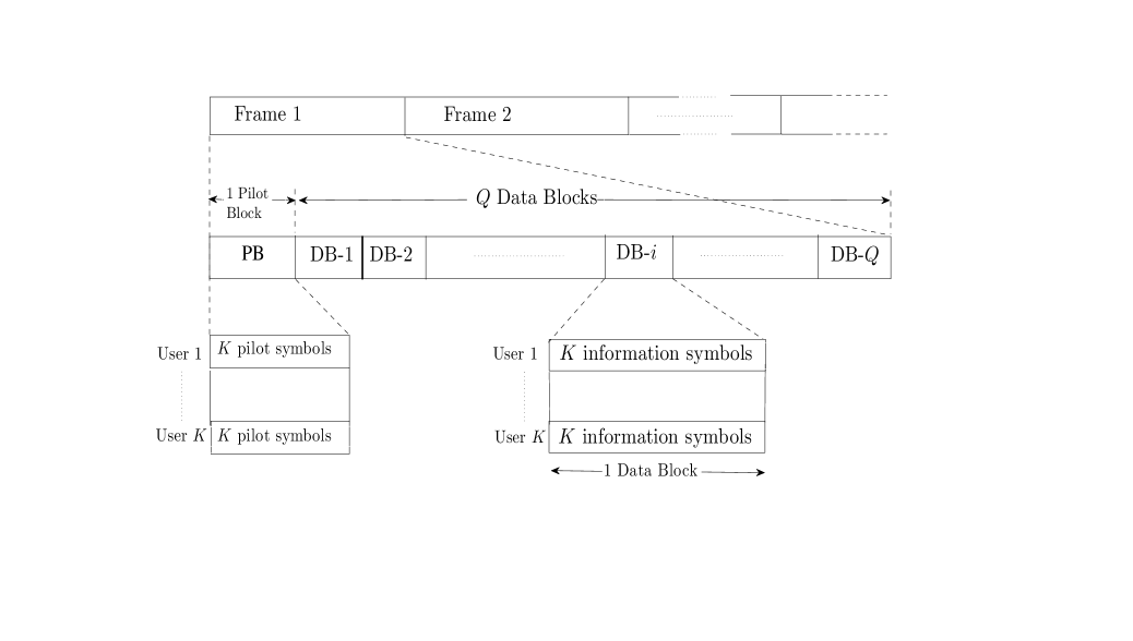
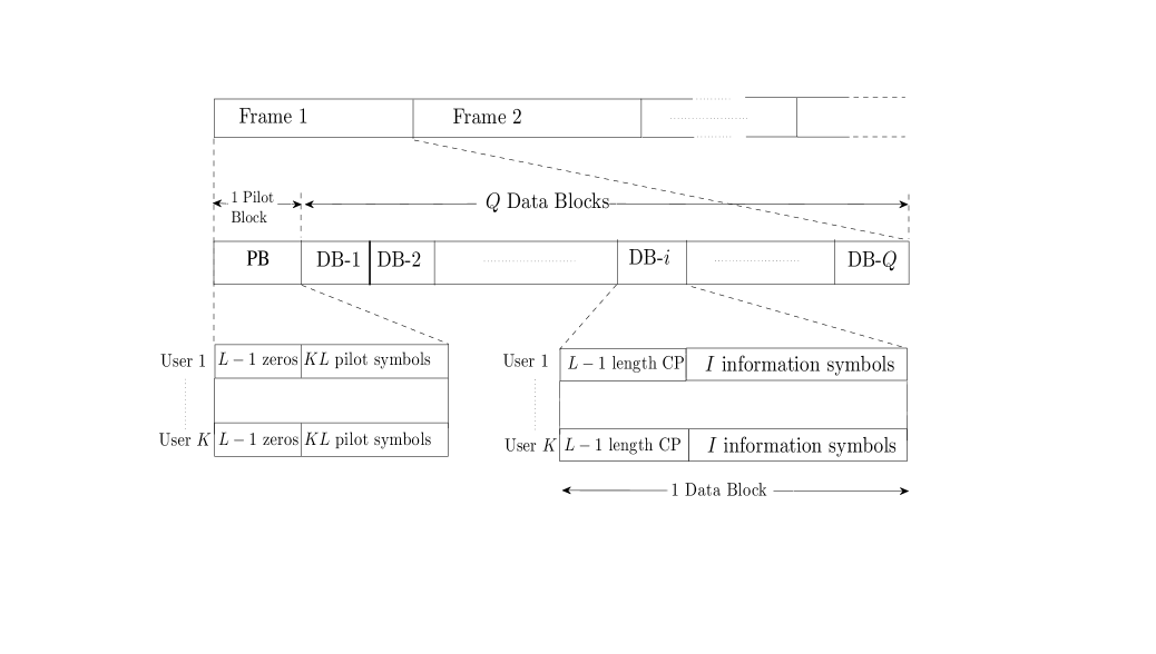
Consider the uplink multiuser MIMO system model in (1). As in Sec. II, perfect synchronization among users’ transmissions is assumed. But the assumption of perfect knowledge of the channel matrix at the BS is relaxed here. The channel matrix is estimated based on a pilot based channel estimation scheme. Transmission is carried out in frames, where each frame consists of several blocks as shown in Fig. 13. A slow fading channel (typical with no/low mobility users) is assumed, where the channel is assumed to be constant over one frame duration. Each frame consists of a pilot block (PB) for the purpose of initial channel estimation, followed by $Q$ data blocks (DB). The pilot block consists of $K$ channel uses in which a $K$-length pilot symbol vector comprising of pilot symbols transmitted from $K$ users (one pilot symbol per user) is received by $N$ receive antennas at the BS. Each data block consists of $K$ channel uses, where $K$ number of $K$-length information symbol vectors (one data symbol from each user) are transmitted. Taking both pilot and data channel uses into account, the total number of channel uses per frame is $(Q+1)K$. Data blocks are detected using the R-MCMC-R algorithm using an initial channel estimate. The detected data blocks are iteratively used to refine the channel estimates during data phase using the proposed MCMC based channel estimation algorithm.

IV-B Initial channel estimate during pilot phase

Let ${\bf x}_{\text{P}}^{k}=[x_{\text{P}}^{k}(0),x_{\text{P}}^{k}(1),\cdots,x_{\text{P}}^{k}(K-1)]$ denote the the pilot symbol vector transmitted from user $k$ in $K$ channel uses in a frame. Let ${\bf X}_{\text{P}}=[({\bf x}_{\text{P}}^{1})^{T},({\bf x}_{\text{P}}^{2})^{T},\cdots,({\bf x}_{\text{P}}^{K})^{T}]^{T}$ denote the $K\times K$ pilot matrix formed by the pilot symbol vectors transmitted by the users in the pilot phase. The received signal matrix at the BS, ${\bf Y}_{\text{P}}$, of size $N\times K$ is given by

$${\bf Y}_{\text{P}}={\bf H}_{c}{\bf X}_{\text{P}}+{\bf N}_{\text{P}},$$ (12)

where ${\bf N}_{\text{P}}$ is the $N\times K$ noise matrix at the BS. We use the pilot sequence given by

$$\mathbf{\bf x}_{\text{P}}^{k}=[\mathbf{0}_{(k-1)\times 1}\quad p\quad\mathbf{0}_{(K-k)\times 1}].$$ (13)

We choose $p=\sqrt{KE_{s}}$, where $E_{s}$ is the average symbol energy. Using the scaled identity nature of ${\bf x}_{\text{P}}$, an initial channel estimate $\widehat{{\bf H}}_{c}$ is obtained as

$$\widehat{{\bf H}}_{c}={\bf Y}_{\text{P}}/p.$$ (14)

IV-C Data detection using initial channel estimate

Let ${\bf x}_{i}^{k}=[x_{i}^{k}(0),x_{i}^{k}(1),\cdots,x_{i}^{k}(K-1)]$ denote the data symbol vector transmitted from user $k$ in $K$ channel uses during the $i$th data block in a frame. Let ${\bf X}_{i}=[({\bf x}_{i}^{1})^{T},({\bf x}_{i}^{2})^{T},\cdots,({\bf x}_{i}^{K})^{T}]^{T}$ denote the $K\times K$ data matrix formed by the data symbol vectors transmitted by the users in the $i$th data block during data phase, $i=1,2,\cdots,Q$. The received signal matrix at the BS in the $i$th data block, ${\bf Y}_{i}$ of size $N\times K$, is given by

$${\bf Y}_{i}={\bf H}_{c}{\bf X}_{i}+{\bf N}_{i},$$ (15)

where ${\bf N}_{i}$ is the $N\times K$ noise matrix at the BS during $i$th data block. We perform the detection on a vector by vector basis using the independence of data symbols transmitted by the users. Let ${\bf y}_{i}^{(t)}$ denote the $t$th column of ${\bf Y}_{i}$, $t=0,2,\cdots,K-1$. Denoting the $t$th column of ${\bf X}_{i}$ as ${\bf x}_{i}^{(t)}=[x_{i}^{1}(t),x_{i}^{2}(t),\cdots,x_{i}^{K}(t)]^{T}$, we can rewrite the system equation (12) as

$${\bf y}_{i}^{(t)}={\bf H}_{c}{\bf x}_{i}^{(t)}+{\bf n}_{i}^{(t)},$$ (16)

where ${\bf n}_{i}^{(t)}$ is the $t$th column of ${\bf N}_{i}$. The initial channel estimate $\widehat{{\bf H}}_{c}$ obtained from (14) is used to detect the transmitted data vectors using the R-MCMC-R algorithm presented in Sec. III.

From (12) and (14), we observe that $\widehat{{\bf H}}_{c}={\bf H}_{c}+{\bf N}_{\text{P}}/p$. This knowledge about imperfection of channel estimates is used to calculate the statistics of error-free ML cost required in the R-MCMC-R algorithm. In Sec. III, we have observed that in case of perfect channel knowledge, the error-free ML cost is nothing but $\|{\bf n}^{2}\|$. In case of imperfect channel knowledge at the receiver, at channel use $t$,

$$\|{\bf y}_{i}^{(t)}-\widehat{{\bf H}}_{c}{\bf x}_{i}^{(t)}\|^{2}=\|{\bf n}_{i}^{(t)}-{\bf N}_{\text{P}}{\bf x}_{i}^{(t)}/p\|^{2}.$$

Each entry of the vector ${\bf n}_{i}^{(t)}-{\bf N}_{\text{P}}{\bf x}_{i}^{(t)}/p$ has mean zero and variance $2\sigma^{2}$. Using this knowledge at the receiver, we detect the transmitted data using R-MCMC-R algorithm and obtain ${\bf\widehat{x}}_{i}^{(t)}$. Let the detected data matrix in data block $i$ be denoted as ${\bf\widehat{X}}_{i}$ = $[{\bf\widehat{x}}_{i}^{(0)}$, ${\bf\widehat{x}}_{i}^{(1)}$, $\cdots$, ${\bf\widehat{x}}_{i}^{(K-1)}]$.

IV-D Channel estimation using MCMC algorithm in data phase

Let ${\bf Y}_{tot}=[{\bf Y}_{\text{P}}\,{\bf Y}_{1}\,{\bf Y}_{2}\,\cdots\,{\bf Y}_{Q}]$, ${\bf X}_{tot}=[{\bf X}_{\text{P}}\,{\bf X}_{1}\,{\bf X}_{2}\,\cdots\,{\bf X}_{Q}]$, and ${\bf N}_{tot}=[{\bf N}_{\text{P}}\,{\bf N}_{1}\,{\bf N}_{2}\,\cdots\,{\bf N}_{Q}]$ denote the matrices corresponding to one full frame. We can express ${\bf Y}_{tot}$ as

$${\bf Y}_{tot}={\bf H}_{c}{\bf X}_{tot}+{\bf N}_{tot}.$$ (17)

This system model corresponding to the full frame is converted into a real-valued system model as done in Sec. II. That is, (17) can be written in the form

$${\bf Y}={\bf H}{\bf X}+{\bf N},$$ (18)

where

$${\bf Y}=\left[\begin{array}[]{cc}\Re({\bf Y}_{tot})\hskip 5.69054pt-\Im({\bf Y}_{tot})\\ \Im({\bf Y}_{tot})\hskip 14.22636pt\Re({\bf Y}_{tot})\end{array}\right],\quad{\bf H}=\left[\begin{array}[]{cc}\Re({\bf H}_{c})\hskip 5.69054pt-\Im({\bf H}_{c})\\ \Im({\bf H}_{c})\hskip 14.22636pt\Re({\bf H}_{c})\end{array}\right],$$

$${\bf X}=\left[\begin{array}[]{cc}\Re({\bf X}_{tot})\hskip 5.69054pt-\Im({\bf X}_{tot})\\ \Im({\bf X}_{tot})\hskip 14.22636pt\Re({\bf X}_{tot})\end{array}\right],\quad{\bf N}=\left[\begin{array}[]{cc}\Re({\bf N}_{tot})\hskip 5.69054pt-\Im({\bf N}_{tot})\\ \Im({\bf N}_{tot})\hskip 14.22636pt\Re({\bf N}_{tot})\end{array}\right].$$

Equation (18) can be written as

$${\bf Y}^{T}={\bf X}^{T}{\bf H}^{T}+{\bf N}^{T}.$$ (19)

Vectorizing the matrices ${\bf Y}^{T}$, ${\bf H}^{T}$, and ${\bf N}^{T}$, we define

$${\bf r}\stackrel{{\scriptstyle\triangle}}{{=}}vec({\bf Y}^{T}),\quad{\bf g}\stackrel{{\scriptstyle\triangle}}{{=}}vec({\bf H}^{T}),\quad{\bf z}\stackrel{{\scriptstyle\triangle}}{{=}}vec({\bf N}^{T}).\quad$$

With the above definitions, (19) can be written in vector form as

$${\bf r}=\underbrace{{\mathbf{I}}_{2N}\otimes{\bf X}^{T}}_{\stackrel{{\scriptstyle\triangle}}{{=}}\,{\mathbf{S}}}\,{\bf g}+{\bf z}.$$ (20)

Now, our goal is to estimate ${\bf g}$ knowing ${\bf r}$, estimate of ${\mathbf{S}}$ and the statistics of ${\bf z}$ using an MCMC approach. The estimate of ${\mathbf{S}}$ is obtained as

$$\widehat{{\bf S}}={\mathbf{I}}_{2N}\otimes{\bf\widehat{X}}^{T},$$

where $\widehat{{\bf X}}=\left[\begin{array}[]{cc}\Re(\widehat{{\bf X}}_{tot})\hskip 5.69054pt-\Im(\widehat{{\bf X}}_{tot})\\ \Im(\widehat{{\bf X}}_{tot})\hskip 14.22636pt\Re(\widehat{{\bf X}}_{tot})\end{array}\right]$ and ${\bf\widehat{X}}_{tot}=[{\bf X}_{\text{P}}\,{\bf\widehat{X}}_{1}\,{\bf\widehat{X}}_{2}\,\cdots\,{\bf\widehat{X}}_{Q}]$. The initial vector for the MCMC algorithm is obtained as

$$\widehat{{\bf g}}^{(0)}=vec(\widehat{{\bf H}}^{T}),$$ (21)

where

$$\widehat{{\bf H}}=\left[\begin{array}[]{cc}\Re(\widehat{{\bf H}}_{c})\hskip 5.69054pt-\Im(\widehat{{\bf H}}_{c})\\ \Im(\widehat{{\bf H}}_{c})\hskip 14.22636pt\Re(\widehat{{\bf H}}_{c})\end{array}\right].$$ (22)

IV-D1 Gibbs sampling based estimation

The vector ${\bf g}$ is of length $4KN\times 1$. To estimate ${\bf g}$, the algorithm starts with an initial estimate, takes samples from the conditional distribution of each coordinate in ${\bf g}$, and updates the estimate. This is carried out for a certain number of iterations. At the end of the iterations, a weighted average of the previous and current estimates are given as the output.

Let the $i$th coordinate in ${\bf g}$ be denoted by $g_{i}$, and let ${\bf g}_{-i}$ denote all elements in ${\bf g}$ other than the $i$th element. Let $\widehat{\bf s}_{q}$ denote the $q$th column of $\widehat{{\bf S}}$. The conditional probability distribution for the $i$th coordinate is given by

$$p\left(g_{i}|{\bf r},{\bf\widehat{S}},{\bf g}_{-i}\right) \propto p(g_{i}).\,p\left({\bf r}|g_{i},{\bf\widehat{S}},{\bf g}_{-i}\right)$$ (23)

$$\propto \exp\left(-|g_{i}|^{2}\right)\exp\left(-\frac{\|{\bf r}-\sum_{q=1,q\not=i}^{4KN}g_{q}{\bf\widehat{s}}_{q}-g_{i}{\bf\widehat{s}}_{i}\|^{2}}{\sigma^{2}}\right)$$ (24)

$$= \exp\left(-|g_{i}|^{2}-\frac{\|{\widetilde{\bf r}}^{(i)}-g_{i}{\bf\widehat{s}}_{i}\|^{2}}{\sigma^{2}}\right)$$ (25)

$$= \exp\left(-\frac{\|\bar{{\bf r}}^{(i)}-g_{i}{\bf\bar{s}}_{i}\|^{2}}{\sigma^{2}}\right),$$ (26)

where ${\widetilde{\bf r}}^{(i)}={\bf r}-\sum_{q=1,q\not=i}^{4KN}g_{q}{\bf\widehat{s}}_{q}$, $\bar{{\bf r}}^{(i)}=[{\widetilde{\bf r}}^{(i)},\,0]^{T}$, and ${\bf\bar{s}}_{i}=[{\bf\widehat{s}}_{i},\,\sigma]^{T}$. The quantity $\|\bar{{\bf r}}^{(i)}-g_{i}{\bf\bar{s}}_{i}\|^{2}$ in (26) is minimized for $g_{i}=\frac{\left(\bar{{\bf r}}^{(i)}\right)^{T}{\bf\bar{s}}_{i}}{\|\bar{{\bf s}}_{i}\|^{2}}$. Hence, we can write

$$\|\bar{{\bf r}}^{(i)}-g_{i}{\bf\bar{s}}_{i}\|^{2} = \|\bar{{\bf r}}^{(i)}-\left(\frac{\left(\bar{{\bf r}}^{(i)}\right)^{T}{\bf\bar{s}}_{i}}{\|\bar{{\bf s}}_{i}\|^{2}}+g_{i}-\frac{\left(\bar{{\bf r}}^{(i)}\right)^{T}{\bf\bar{s}}_{i}}{\|\bar{{\bf s}}_{i}\|^{2}}\right){\bf\bar{s}}_{i}\|^{2}$$ (27)

$$= \|\bar{{\bf r}}^{(i)}-\frac{\left(\bar{{\bf r}}^{(i)}\right)^{T}{\bf\bar{s}}_{i}}{\|\bar{{\bf s}}_{i}\|^{2}}{\bf\bar{s}}_{i}\|^{2}+\left(g_{i}-\frac{\left(\bar{{\bf r}}^{(i)}\right)^{T}{\bf\bar{s}}_{i}}{\|\bar{{\bf s}}_{i}\|^{2}}\right)^{2}\|{\bf\bar{s}}_{i}\|^{2}.$$

Hence,

$$p\left(g_{i}|{\bf r},{\bf\widehat{S}},{\bf g}_{-i}\right) \propto \exp\left(-\frac{\Big{(}g_{i}-\frac{\left(\bar{{\bf r}}^{(i)}\right)^{T}{\bf\bar{s}}_{i}}{\|\bar{{\bf s}}_{i}\|^{2}}\Big{)}^{2}}{\frac{\sigma^{2}}{\|{\bf s}_{i}\|^{2}}}\right).$$ (28)

This distribution is Gaussian with mean

$$\mu_{g_{i}}=\frac{\left(\bar{{\bf r}}^{(i)}\right)^{T}{\bf\bar{s}}_{i}}{\|\bar{{\bf s}}_{i}\|^{2}},$$ (29)

and variance

$$\sigma_{g_{i}}^{2}=\frac{\sigma^{2}}{2\|{\bf s}_{i}\|^{2}}.$$ (30)

Let $MAX$ denote the number of MCMC iterations. In each MCMC iteration, for each coordinate, the probability distribution specified by its mean and variance has to be calculated to draw samples. Let the mean and variance in $r$th MCMC iteration and $i$th coordinate be denoted as $\mu_{g_{i}}^{(r)}$ and ${\sigma_{g_{i}}^{2}}^{(r)}$, respectively, where $r=1,2,\cdots,MAX$ and $i=1,2,\cdots,4KN$. We use $\widehat{{\bf g}}^{(0)}$in (21), which is the estimate from the pilot phase, as the initial estimate. In the $r$th MCMC iteration, we obtain $\widehat{{\bf g}}^{(r)}$ from $\widehat{{\bf g}}^{(r-1)}$ as follows:

• Take $\widehat{{\bf g}}^{(r)}=\widehat{{\bf g}}^{(r-1)}$.

• Update the $i$th coordinate of $\widehat{{\bf g}}^{(r)}$ by sampling from $\mathcal{N}\Big{(}\mu_{g_{i}}^{(r)}$, ${\sigma_{g_{i}}^{2}}^{(r)}\Big{)}$ for all $i$. Let $\widehat{g}^{(r)}_{i}$ denote the updated $i$th coordinate of ${\bf g}^{(r)}$.

• Compute weights $\alpha_{i}^{(r)}=\exp\left(-\frac{\left(\widehat{g}^{(r)}_{i}-\mu_{g_{i}}^{(r)}\right)^{2}}{2{\sigma_{g_{i}}^{2}}^{(r)}}\right)$ for all $i$. This gives more weight to samples closer to the mean.

After $MAX$ iterations, we compute the final estimate of the $i$th coordinate, denoted by $g_{i}^{*}$, to be the following weighted sum of the estimates from previous and current iterations:

$$g_{i}^{*}=\frac{\sum_{r=1}^{MAX}\alpha_{i}^{(r)}\widehat{g}^{(r)}_{i}}{\sum_{r=1}^{MAX}\alpha_{i}^{(r)}}.$$ (31)

Finally, the updated $2N\times 2K$ channel estimate ${\widehat{{\bf H}}}$ is obtained by restructuring ${\bf g}^{*}=[g_{1}^{*},g_{2}^{*},\cdots,g_{4KN}^{*}]^{T}$ as follows:

$${\widehat{{\bf H}}}(p,q)=g_{n}^{*},\quad p=1,2,\cdots,2N,\quad q=1,2,\cdots,2K,$$ (32)

where $n=2N(p-1)+q$ and $\widehat{{\bf H}}(p,q)$ denotes the element in the $p$th row and $q$th column of $\widehat{{\bf H}}$. A complete listing of the proposed MCMC algorithm for channel estimation is given in the next page.

The matrix $\widehat{{\bf H}}$ obtained thus is used for data detection using R-MCMC-R algorithm. This ends one iteration between channel estimation and detection. The detected data matrix is fed back for channel estimation in the next iteration, whose output is then used to detect the data matrix again. This iterative channel estimation and detection procedure is carried out for a certain number of iterations.

Algorithm 2 Proposed MCMC algorithm for channel estimation

1:  input: ${\bf r}$, , $\widehat{{\mathbf{S}}}$, $\sigma^{2}$, $\widehat{{\bf g}}^{(0)}:$ initial vector $\in{\mathbb{R}}^{4KN}$;    $MAX$: max. # iterations;

2:  $r=1$;    $g^{*}(0)=\widehat{{\bf g}}^{(0)}$;    $\alpha_{i}^{(0)}=0$, $\forall i=1,2,\cdots,4KN$;

3:  while $r<MAX$ do

4:      $\widehat{{\bf g}}^{(r)}=\widehat{{\bf g}}^{(r-1)}$;

5:     ${\widetilde{\bf r}}^{*}={\bf r}-\widehat{{\mathbf{S}}}\widehat{{\bf g}}^{(r)}$;

6:     for $i=1$ to $4KN$ do

7:        Compute ${\widetilde{\bf r}}^{(i)}={\widetilde{\bf r}}^{*}+\widehat{g}_{i}^{(r)}{\bf\widehat{s}}_{i}$, $\bar{{\bf r}}^{(i)}=[{\widetilde{\bf r}}^{(i)},\,0]^{T}$, and ${\bf\bar{s}}_{i}=[{\bf\widehat{s}}_{i},\,\sigma]^{T}$;

8:        Compute $\mu_{g_{i}}^{(r)}=\frac{\left(\bar{{\bf r}}^{(i)}\right)^{T}{\bf\bar{s}}_{i}}{\|\bar{{\bf s}}_{i}\|^{2}}$ and ${\sigma_{g_{i}}^{2}}^{(r)}=\frac{\sigma^{2}}{2\|{\bf s}_{i}\|^{2}}$;

9:        Sample $\widehat{g}_{i}^{(r)}\thicksim\mathcal{N}\Big{(}\mu_{g_{i}}^{(r)}$, ${\sigma_{g_{i}}^{2}}^{(r)}\Big{)}$;

10:        ${\widetilde{\bf r}}^{*}={\widetilde{\bf r}}^{(i)}-\widehat{g}_{i}^{(r)}{\bf\widehat{s}}_{i}$;

11:        Compute $\alpha_{i}^{(r)}=\exp\left(-\frac{\left(\widehat{g}^{(r)}_{i}-\mu_{g_{i}}^{(r)}\right)^{2}}{2{\sigma_{g_{i}}^{2}}^{(r)}}\right)$;

12:        $g_{i}^{*}(r)=\frac{\alpha_{i}^{(r)}\widehat{g}^{(r)}_{i}+\left(\sum_{z=o}^{r-1}\alpha_{i}^{(z)}\right)g_{i}^{*}(r-1)}{\sum_{z=0}^{r}\alpha_{i}^{(z)}}$;

13:     end for

14:     $r=r+1$;

15:  end while

16:  output: ${\bf g}^{*}={\bf g}^{*}(MAX).\qquad{\bf g}^{*}:$ output solution vector

IV-E Performance Results

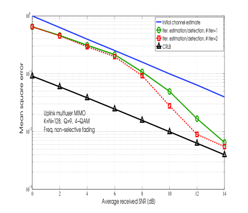
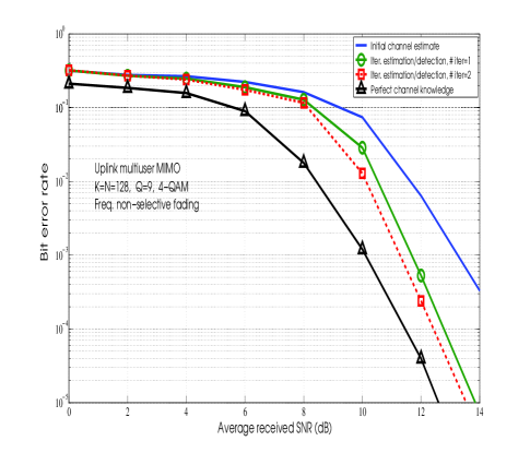
In Fig. 14(a), we plot the mean square error performance (MSE) of the iterative channel estimation/detection scheme using proposed MCMC based channel estimation and R-MCMC-R based detection with 4-QAM for $K=N=128$ and $Q=9$. In the simulations, the R-MCMC-R algorithm parameter values used are the same as in Sec. III-C4. For the MCMC channel estimation algorithm, the value of MAX used is 2. The MSEs of the initial channel estimate, and the channel estimates after 1 and 2 iterations between channel estimation and detection are shown. For comparison, we also plot the Cramer-Rao lower bound (CRLB) for this system. It can be seen that in the proposed scheme results in good MSE performance with improved MSE for increased number of iterations between channel estimation and detection. For the same set of system and algorithm parameters in Fig. 14(a), we plot the BER performance curves in Fig. 14(b). For comparison, we also plot the BER performance with perfect channel knowledge. It can be seen that with two iterations between channel estimation and detection the proposed MCMC based algorithms can achieve $10^{-3}$ BER within about 1 dB of the performance with perfect channel knowledge.

V Equalization/Channel Estimation in Frequency Selective Fading

In the previous sections, we considered frequency non-selective fading. In this section, we consider equalization and channel estimation in frequency selective fading. Multicarrier techniques like OFDM can transform a frequency selective channel into several narrow-band frequency non-selective channels. The MCMC based algorithms proposed in the previous sections can be employed for signal detection and channel estimation on the resulting narrow-band channels. However, multicarrier systems face the peak-to-average power ratio (PAPR) problem. Single carrier (SC) block transmission schemes are considered as good alternatives to address the PAPR issue that arises in multicarrier systems [39]-[45]. We consider cyclic prefixed single-carrier (CPSC) signaling, where the overall channel includes a Fourier transform (FFT) operation so that the transmitted symbols are estimated from the received frequency-domain signal [39],[40],[41]. In [46], the optimal training sequence that minimizes the channel estimation mean square error of the linear channel estimator is shown to be of length $KL$ per transmit antenna. Blind/semi-blind channel estimation methods can be considered, but they require long data samples and the complexity is high [47],[48]. Here, we consider channel estimation using uplink pilots and iterations between channel estimation and equalization in multiuser MIMO CPSC systems.

V-A Multiuser MIMO CPSC system model

Consider the uplink multiuser MIMO system shown in Fig. 1. The channel between each pair of user transmit antenna and BS receive antenna is assumed to be frequency selective with L multipath components. Let $h^{(j,k)}(l)$ denote the channel gain between $k$th user and $j$th receive antenna at the BS on the $l$th path, which is modeled as $\mathcal{CN}(0,\Omega_{l}^{2})$. As in Sec. II, perfect synchronization among users’ transmissions is assumed. Transmission is carried out in frames, where each frame consists of several blocks as shown in Fig. 15. As in IV-A, the channel is assumed to be constant over one frame duration. Each frame consists of a pilot block for the purpose of initial channel estimation, followed by $Q$ data blocks. The pilot block consists of $(L-1)+KL$ channel uses. In the first $L-1$ channel uses in the pilot block, padding of $L-1$ zeros is used to avoid inter-frame interference. In each of the remaining $KL$ channel uses, a $K$-length pilot symbol vector comprising of pilot symbols transmitted from $K$ users (one pilot symbol per user) is received by $N$ receive antennas at the BS. Each data block consists of $I+L-1$ channel uses, where $I$ number of $K$-length information symbol vectors (one data symbol from each user) preceded by $(L-1)$-length cyclic prefix from each user (to avoid inter-block interference) are transmitted. With $Q$ data blocks in a frame, the number of channel uses in the data part of the frame is $(I+L-1)Q$. Taking both pilot and data channel uses into account, the total number of channel uses per frame is $(L+1)K+(I+L-1)Q-1$. Data blocks are detected using the R-MCMC-R algorithm using an initial channel estimate. The detected data blocks are then iteratively used to refine the channel estimates during data phase. The padding of $L-1$ zeros at the beginning of the pilot block makes the transmitters silent during the first $L-1$ channel uses in a frame. The channel output in these channel uses are ignored at the receiver. Accordingly, the 0th channel use in a frame at the receiver is taken to be the channel use in which the first pilot symbol in the frame is sent.

V-B Initial channel estimate during pilot phase

Let $\mathbf{b}^{k}=[b^{k}(0),b^{k}(1),\cdots,b^{k}(KL-1)]$ denote the pilot symbol vector transmitted from user $k$ in $KL$ channel uses in a frame. The signal received by the $j$th receive antenna at the BS during pilot phase in the $n$th channel use is given by

$$y_{\text{P}}^{j}(n)=\sum_{k=1}^{K}\sum_{l=0}^{L-1}h^{(j,k)}(l)b^{k}(n-l)+{q}_{\text{P}}^{j}(n),$$ (33)

$j=1,2\cdots,N$, $n=0,1,\cdots,KL-1$, where the subscript P in ${y}_{\text{P}}^{j}(n)$ and ${q}_{\text{P}}^{j}(n)$ denotes pilot phase. $\{{q}_{\text{P}}^{j}(n)\}$ are noise samples modeled as i.i.d. $\mathcal{CN}(0,\sigma^{2})$. We use the training sequence given by

$$\mathbf{b}^{k}=[\mathbf{0}_{(k-1)L\times 1}\quad b\quad\mathbf{0}_{(K-(k-1))L-1)\times 1}].$$ (34)

Writing (33) in matrix notation after substituting (34), we get

$$\mathbf{y}_{\text{P}}^{j}=\mathbf{B}_{\text{P}}\mathbf{h}^{j}+\mathbf{q}_{\text{P}}^{j},\quad j=1,2,\cdots,N,$$ (35)

where

$$\mathbf{y}_{\text{P}}^{j}=[y_{\text{P}}^{j}(0),y_{\text{P}}^{j}(1),\cdots,y_{\text{P}}^{j}(KL-1)]^{T},\quad\quad\mathbf{h}^{j}=[(\mathbf{h}^{(j,1)})^{T},\cdots,(\mathbf{h}^{(j,k)})^{T},\cdots,(\mathbf{h}^{(j,K)})^{T}]^{T},$$

$$\mathbf{h}^{(j,k)}=[h^{(j,k)}(0),h^{(j,k)}(1),\cdots,h^{(j,k)}(L-1)]^{T},\quad\quad\mathbf{q}_{\text{P}}^{j}=[q_{\text{P}}^{j}(0),q_{\text{P}}^{j}(1),\cdots,q_{\text{P}}^{j}(KL-1)]^{T},$$

$$\mathbf{B}_{\text{P}}=[\mathbf{B}_{{\text{p}}_{1}}\mathbf{B}_{{\text{P}}_{2}}\cdots\mathbf{B}_{{\text{P}}_{K}}],\quad\quad\mathbf{B}_{{\text{P}}_{k}}=[\mathbf{0}_{L\times(k-1)L}\quad b\mathbf{I}_{L}\quad\mathbf{0}_{L\times(K-k)L}]^{T}.$$

We use $b=\sqrt{KE_{s}\left(\sum_{l=0}^{L-1}\Omega_{l}^{2}\right)}$ to maintain the same average receive SNR in both pilot phase and data phase.

From the signal observed at the $j$th receive antenna from time $0$ to $KL-1$ during pilot phase, we obtain an initial estimate the channel vector ${\bf h}^{j}$ using the scaled identity nature of $\mathbf{B}_{\text{P}}$, as

$$\mathbf{\widehat{h}}^{j}=\mathbf{y}_{\text{P}}^{j}/b,\quad j=1,2,\cdots,N.$$ (36)

These initial channel estimates are used to detect the data vectors in the data phase.

V-C Equalization using initial channel estimates

In the data phase, let $\mathbf{a}_{i}^{k}=[{a}_{i}^{k}(0),{a}_{i}^{k}(1),\cdots,{a}_{i}^{k}(I+L-2)]^{T}$ denote the data vector of size $(I+L-1)\times 1$, which includes $(L-1)$ cyclic prefix symbols and $I$ information symbols transmitted from $k$th user during $i$th data block, $i=1,2,\cdots,Q$. The signal received at $j$th receive antenna at $n$th channel use of $i$th data block is given by

$$y_{i}^{j}(n)=\sum_{k=1}^{K}\sum_{l=0}^{L-1}h^{(j,k)}(l)a^{k}_{i}(n-l)+q_{i}^{j}(n),$$ (37)

$j=1,2\cdots,N,\,n=0,1,\cdots,I+L-2$, where ${q}_{i}^{j}(n)$ is the noise sample modeled as i.i.d. $\mathcal{CN}(0,\sigma^{2})$. Define the following vectors and matrices: $\mathbf{y}_{i}^{j}\stackrel{{\scriptstyle\triangle}}{{=}}[y_{i}^{j}(L-1),y_{i}^{j}(L),\cdots,y_{i}^{j}(I+L-2)]^{T}$, $\mathbf{q}_{i}^{j}\stackrel{{\scriptstyle\triangle}}{{=}}[q_{i}^{j}(L-1),q_{i}^{j}(L),\cdots,q_{i}^{j}(I+L-2)]^{T}$, $\mathbf{x}_{i}^{k}\stackrel{{\scriptstyle\triangle}}{{=}}[{a}_{i}^{k}(L-1),{a}_{i}^{k}(L),\cdots,{a}_{i}^{k}(I+L-2)]^{T}$, and $\mathbf{H}^{j,k}$ as a $(I+L)\times I$ circulant matrix with $[h^{(j,k)}(0),h^{(j,k)}(1),\cdots,h^{(j,k)}(L-1),0,\cdots,0]^{T}$ as the first column. With these definitions, (37) can be written in the form

$$\mathbf{y}_{i}^{j}=\sum_{k=1}^{K}\mathbf{H}^{j,k}\mathbf{x}_{i}^{k}+\mathbf{q}_{i}^{j},\quad j=1,2,\cdots,N.$$ (38)

We can write (38) as

$$\mathbf{y}_{i}=\mathbf{H}\mathbf{x}_{i}+\mathbf{q}_{i},\quad i=1,2,\cdots,Q,$$ (39)

where $\mathbf{y}_{i}=[(\mathbf{y}_{i}^{1})^{T},(\mathbf{y}_{i}^{2})^{T},\cdots,(\mathbf{y}_{i}^{N})^{T}]^{T}$, $\mathbf{x}_{i}=[(\mathbf{x}_{i}^{1})^{T},(\mathbf{x}_{i}^{2})^{T},\cdots,(\mathbf{x}_{i}^{K})^{T}]^{T}$, $\mathbf{q}_{i}=[(\mathbf{q}_{i}^{1})^{T},(\mathbf{q}_{i}^{2})^{T},\cdots,(\mathbf{q}_{i}^{N})^{T}]^{T}$, and

$$\mathbf{H}=\left[\begin{array}[]{ccc}\mathbf{H}^{1,1}&\mathbf{H}^{1,2}\cdots&\mathbf{H}^{1,K}\\ \mathbf{H}^{2,1}&\mathbf{H}^{2,2}\cdots&\mathbf{H}^{2,K}\\ \vdots&\vdots&\vdots\\ \mathbf{H}^{N,1}&\mathbf{H}^{N,2}\cdots&\mathbf{H}^{N,K}\\ \end{array}\right].$$

V-C1 Equalization using R-MCMC-R method

The R-MCMC-R algorithm proposed in Sec. III is employed in the frequency domain using FFT based processing for equalization. The circulant matrix $\mathbf{{H}}^{j,k}$ can be decomposed as

$$\mathbf{H}^{j,k}=\mathbf{F}_{I}^{H}\mathbf{D}^{j,k}\mathbf{F}_{I},$$ (40)

where $\mathbf{F}_{I}$ is $I\times I$ DFT matrix, and $\mathbf{D}^{j,k}$ is a diagonal matrix with its diagonal elements to be the DFT of the vector $[h^{(j,k)}(0),h^{(j,k)}(1),\cdots,h^{(j,k)}(L-1),0,\cdots,0]^{T}$. Taking the DFT of $\mathbf{{y}}_{i}^{j}$ in (38), we get

$$\mathbf{z}_{i}^{j}=\mathbf{F}_{I}\mathbf{{y}}_{i}^{j}=\sum_{k=1}^{K}\mathbf{D}^{j,k}\mathbf{{b}}_{i}^{k}+\mathbf{w}_{i}^{j},\quad j=1,2,\cdots,N,$$ (41)

where $\mathbf{z}_{i}^{j}=[z_{i}^{j}(0),z_{i}^{j}(1),\cdots,z_{i}^{j}(I-1)]^{T}$,  $\mathbf{{b}}_{i}^{k}\stackrel{{\scriptstyle\triangle}}{{=}}\mathbf{F}_{I}\mathbf{x}_{i}^{k}=[b_{i}^{k}(0),b_{i}^{k}(1),\cdots,b_{i}^{k}(I-1)]^{T}$, and $\mathbf{w}_{i}^{j}\stackrel{{\scriptstyle\triangle}}{{=}}\mathbf{F}_{I}\mathbf{{q}}_{i}^{j}=[w_{i}^{j}(0),w_{i}^{j}(1),\cdots,w_{i}^{j}(I-1)]^{T}$. Writing (41) in matrix form, we get

$$\mathbf{z}_{i}=\mathbf{D}\mathbf{{b}}_{i}+\mathbf{w}_{i},\quad i=1,2,\cdots,Q,$$ (42)

where $\mathbf{z}_{i}=[(\mathbf{z}_{i}^{1})^{T},(\mathbf{z}_{i}^{2})^{T},\cdots,(\mathbf{z}_{i}^{N})^{T}]^{T}$, $\mathbf{{b}}_{i}=[(\mathbf{{b}}_{i}^{1})^{T},(\mathbf{{b}}_{i}^{2})^{T},\cdots,(\mathbf{{b}}_{i}^{K})^{T}]^{T}$, $\mathbf{w}_{i}=[(\mathbf{w}_{i}^{1})^{T},(\mathbf{w}_{i}^{2})^{T},\cdots,(\mathbf{w}_{i}^{N})^{T}]^{T}$, and

$$\mathbf{D}=\left[\begin{array}[]{ccc}\mathbf{D}^{1,1}&\mathbf{D}^{1,2}\cdots&\mathbf{D}^{1,K}\\ \mathbf{D}^{2,1}&\mathbf{D}^{2,2}\cdots&\mathbf{D}^{2,K}\\ \vdots&\vdots&\vdots\\ \mathbf{D}^{N,1}&\mathbf{D}^{N,2}\cdots&\mathbf{D}^{N,K}\\ \end{array}\right].$$

Rearranging the terms, we can also write (42) as

$$\mathbf{\bar{z}}_{i}=\mathbf{\bar{D}}\mathbf{\bar{b}}_{i}+\mathbf{\bar{w}}_{i},\quad i=1,2,\cdots,Q,$$ (43)

where

$$\mathbf{\bar{z}}_{i}=\left[\begin{array}[]{c}\mathbf{\bar{z}}_{i}(0)\\ \mathbf{\bar{z}}_{i}(1)\\ \vdots\\ \mathbf{\bar{z}}_{i}(I-1)\end{array}\right]\mathrm{,}\,\,\mathbf{\bar{b}}_{i}=\left[\begin{array}[]{c}\mathbf{\bar{b}}_{i}(0)\\ \mathbf{\bar{b}}_{i}(1)\\ \vdots\\ \mathbf{\bar{b}}_{i}(I-1)\end{array}\right],\,\,\mathbf{\bar{D}}=\left[\begin{array}[]{ccc}\mathbf{\bar{D}}(0)&\cdots&0\\ \vdots&\ddots&\vdots\\ 0&\cdots&\mathbf{\bar{D}}(I-1)\\ \end{array}\right]\mathrm{,}\,\,\mathbf{\bar{w}}_{i}=\left[\begin{array}[]{c}\mathbf{\bar{w}}_{i}(0)\\ \mathbf{\bar{w}}_{i}(1)\\ \vdots\\ \mathbf{\bar{w}}_{i}(I-1)\end{array}\right],$$

$\mathbf{\bar{z}}_{i}(m)=[{z}_{i}^{1}(m),{z}_{i}^{2}(m),\cdots,{z}_{i}^{N}(m)]^{T}$, $\mathbf{\bar{b}}_{i}(m)=[{b}_{i}^{1}(m),{b}_{i}^{2}(m),\cdots,{b}_{i}^{N}(m)]^{T}$,
$\mathbf{\bar{w}}_{i}(m)=[{w}_{i}^{1}(m),{w}_{i}^{2}(m),\cdots,{w}_{i}^{N}(m)]^{T}$, and

$$\mathbf{\bar{D}}(m)=\left[\begin{array}[]{ccc}\mathbf{D}^{1,1}(m)&\mathbf{D}^{1,2}(m)\cdots&\mathbf{D}^{1,K}(m)\\ \mathbf{D}^{2,1}(m)&\mathbf{D}^{2,2}(m)\cdots&\mathbf{D}^{2,K}(m)\\ \vdots&\vdots&\vdots\\ \mathbf{D}^{N,1}(m)&\mathbf{D}^{N,2}(m)\cdots&\mathbf{D}^{N,K}(m)\\ \end{array}\right].$$

$\mathbf{D}^{j,k}(m)$ is the $m$th diagonal element of the matrix $\mathbf{D}^{j,k}$. Also, $\mathbf{\bar{b}}_{i}=\mathbf{{\bar{F}}}\mathbf{\bar{x}}_{i}$, where $\mathbf{{\bar{F}}}\stackrel{{\scriptstyle\triangle}}{{=}}\mathbf{F}_{I}\otimes\mathbf{I}_{K}$, $\mathbf{\bar{x}}_{i}=[a_{i}^{1}(L-1)\cdots a_{i}^{K}(L-1),a_{i}^{1}(L)\cdots a_{i}^{K}(L),\cdots,a_{i}^{1}(I+L-2)\cdots a_{i}^{K}(I+L-2)]^{T}$. Now, we have

$$\mathbf{\bar{z}}_{i} = \mathbf{\bar{D}}\mathbf{{\bar{F}}}\mathbf{\bar{x}}_{i}+\mathbf{\bar{w}}_{i}$$ (44)

$$= \mathbf{{\bar{H}}}\mathbf{\bar{x}}_{i}+\mathbf{\bar{w}}_{i},\quad i=1,2,\cdots,Q,$$

where $\mathbf{{\bar{H}}}\stackrel{{\scriptstyle\triangle}}{{=}}\mathbf{\bar{D}}\mathbf{{\bar{F}}}$.

For each $i$ in (44), we run R-MCMC-R detection algorithm and detect the information symbols in the $i$th block. In the first iteration of data detection, we use the channel estimates from (36) to calculate $\mathbf{\widehat{{\bar{H}}}}$, an estimate of $\mathbf{{\bar{H}}}$. Each coordinate of the vector $(\mathbf{\bar{z}}_{i}-\mathbf{\widehat{{\bar{H}}}}\mathbf{\bar{x}}_{i})$ has zero mean and $2\sigma^{2}$ variance. Using this knowledge, the statistics of the ML cost of error-free vectors are recalculated in the R-MCMC-R algorithm. R-MCMC-R detector outputs are denoted by $\hat{{\bf x}}_{i}^{k}$, $k=1,\cdots,K$,   $i=1,\cdots,Q$. These output vectors are then used to improve the channel estimates through iterations between equalization and channel estimation. The channel estimation in these iterations is based on MCMC approach presented next.

V-D MCMC based channel estimation in data phase

Consider (41), which can be rewritten as

$$\mathbf{z}_{i}^{j}=\sum_{k=1}^{K}\mathbf{{B}}_{i}^{k}\mathbf{d}^{j,k}+\mathbf{w}_{i}^{j},\quad j=1,2,\cdots,N,$$ (45)

where $\mathbf{{B}}_{i}^{k}=diag(\mathbf{{b}}_{i}^{k})$, $\mathbf{d}^{j,k}$ is a vector consisting of the diagonal elements of matrix $\mathbf{D}^{j,k}$, which is the $I$-point DFT of $\mathbf{h}^{(j,k)}$ (zero padded to length $I$), i.e., $\mathbf{d}^{j,k}=\tilde{\mathbf{F}}_{I\times L}\mathbf{h}^{(j,k)}$, where $\tilde{\mathbf{F}}_{I\times L}$ is the matrix with the first $L$ columns of $\mathbf{F}_{I}$. Now, (45) can be written as

$$\mathbf{z}_{i}^{j}=\sum_{k=1}^{K}\mathbf{{B}}_{i}^{k}\tilde{\mathbf{F}}_{I\times L}\mathbf{h}^{(j,k)}+\mathbf{w}_{i}^{j}.$$ (46)

Defining $\mathbf{{A}}_{i}^{k}\stackrel{{\scriptstyle\triangle}}{{=}}\mathbf{{B}}_{i}^{k}\tilde{\mathbf{F}}_{I\times L}$, we can write (46) as

$$\mathbf{z}_{i}^{j}=\mathbf{{A}}_{i}\mathbf{h}^{j}+\mathbf{w}_{i}^{j},\quad i=1,\cdots,Q,$$ (47)

where $\mathbf{A}_{i}=[\mathbf{{A}}_{i}^{1}\,\mathbf{{A}}_{i}^{2}\,\cdots\,\mathbf{{A}}_{i}^{K}]$. We can write (47) as

$$\mathbf{z}^{j}=\mathbf{{A}}\mathbf{h}^{j}+\mathbf{w}^{j},$$ (48)

where

$$\mathbf{{z}}^{j}=\left[\begin{array}[]{c}\mathbf{{z}}_{1}^{j}\\ \mathbf{{z}}_{2}^{j}\\ \vdots\\ \mathbf{{z}}_{Q}^{j}\end{array}\right],\,\,\mathbf{{A}}=\left[\begin{array}[]{c}\mathbf{{A}}_{1}\\ \mathbf{{A}}_{2}\\ \vdots\\ \mathbf{{A}}_{Q}\end{array}\right],\,\,\mathbf{{w}}^{j}=\left[\begin{array}[]{c}\mathbf{{w}}_{1}^{j}\\ \mathbf{{w}}_{2}^{j}\\ \vdots\\ \mathbf{{w}}_{Q}^{j}\end{array}\right].$$

Using the signal received at antenna $j$ from blocks $1$ to $Q$ in a frame (i.e., using $\mathbf{z}^{j}$) and the matrix $\mathbf{\hat{A}}$ which is formed by replacing the information symbols $\{\mathbf{x}_{i}^{k}\}$ in $\mathbf{A}$ by the detected information symbols $\{\hat{\mathbf{x}}_{i}^{k}\}$, the channel coefficients {$\mathbf{h}^{j}$} are estimated using MCMC based estimation technique presented in Sec. IV-D1. This ends one iteration between channel estimation and detection. The detected data matrix is fed back for channel estimation in the next iteration, whose output is then used to detect the data matrix again. This iterative channel estimation and detection procedure is carried out for a certain number of iterations.

V-E Performance Results

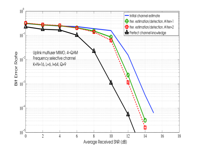
In Fig. 16, we plot the BER performance of the iterative channel estimation/detection scheme using proposed MCMC based channel estimation and R-MCMC-R detection algorithms in uplink multiuser MIMO system on frequency selective fading with $K=N=16,L=6,I=64,Q=9$ and 4-QAM. For the same settings, we also plot the BER performance of the R-MCMC-R algorithm with perfect channel knowledge. BER improves with increasing number of iterations between channel estimation and detection. It can be observed that the proposed scheme with iterations is able to achieve performance which is close to the performance with perfect channel knowledge.

VI Conclusions

We proposed novel MCMC based detection and channel estimation algorithms that achieved near-optimal performance on the uplink in large-scale multiuser MIMO systems. The proposed R-MCMC-R detection algorithm was shown to alleviate the stalling problem and achieve near-ML performance in large systems with tens to hundreds of antennas and higher-order QAM. Key ideas that enabled such attractive performance and complexity include $i)$ a randomized sampling strategy that gave the algorithm opportunities to quickly exit from stalled solutions and move to better solutions, and $ii)$ multiple random restarts that facilitated the algorithm to seek good solutions in different parts of the solution space. Multiple restarts alone (without randomized sampling) could not achieve near-ML performance at low complexity. Randomized sampling alone (without multiple restarts) could achieve near-ML performance at low complexity in the case of 4-QAM. But for higher-order QAM (16-/64-QAM) randomized sampling alone was not adequate. Joint use of both randomized sampling as well as multiple restarts was found to be crucial to achieve near-ML performance for 16-/64-QAM. We also proposed an MCMC based channel estimation algorithm which, in an iterative manner with the R-MCMC-R detection, achieved performance close to performance with perfect channel knowledge. We employed the proposed MCMC receiver architecture in the frequency domain for receiving CPSC signals on frequency selective fading between users and the BS. While simulations were used to establish the attractiveness of the algorithm in performance and complexity, a theoretical analysis that could explain its good performance is important and challenging, which is a topic for future work. We have considered perfect synchronization and single-cell scenario in this paper. Other system level issues including uplink synchronization and multi-cell operation in large-scale MIMO systems can be considered as future work.

Figure 1: Large-scale multiuser MIMO system on the uplink.

Figure 2: BER performance of the proposed R-MCMC algorithm in comparison with those of sphere decoder and MCMC algorithm with different values of $\alpha$ in uplink multiuser MIMO with $K=N=16$, 4-QAM, and no power imbalance. Performance of R-MCMC is almost the same as the sphere decoder performance.

Figure 3: Complexity of the R-MCMC algorithm in average number of real operations per bit as a function of $K=N$ with 4-QAM and no power imbalance at $10^{-2}$ BER.

Figure 4: BER performance of the R-MCMC algorithm in uplink multiuser MIMO with $K=N=8,16,32,64,128$, 4-QAM and no power imbalance.

Figure 5: Average SNR required to achieve $10^{-3}$ BER as a function of number of users $(K=N)$ in uplink multiuser MIMO with 4-QAM and no power imbalance.

Figure 6: BER performance of the R-MCMC algorithm in uplink multiuser MIMO with $K=N=16,128$ and 4-QAM. Power imbalance with $\sigma_{k}^{2}$’s uniformly distributed between -3 dB and 3 dB.

Figure 7: Comparison between R-MCMC performance and sphere decoder performance in uplink multiuser MIMO with $K=N=16$ and 4-/16-/64-QAM.

(a) 4-QAM, SNR=11 dB

(b) 16-QAM, SNR=18 dB

Figure 8: Least ML cost up to $n$th iteration versus $n$ in conventional MCMC and R-MCMC for different initial vectors in multiuser MIMO with $K=N=16$.

Figure 9: BER performance of R-MCMC as a function of number of restarts in multiuser MIMO with $K=N=16$ and 16-QAM at SNR = 18 dB.

(a) 4-QAM

(b) 16-QAM

Figure 10: Histograms of standardized ML costs of correct and incorrect outputs from R-MCMC with restarts in multiuser MIMO with $K=N=8$ and 4-/16-QAM.

Figure 11: BER performance between conventional MCMC (without and with restarts), proposed R-MCMC (without and with restarts), and sphere decoder in uplink multiuser MIMO with $K=N=16$ and 16-QAM.

(a) $K=N=16$

(b) $K=N=32$

Figure 12: BER performance of R-MCMC-R algorithm in uplink multiuser MIMO with $K=N=16$ and $32$ and higher-order modulation (4-/16-/64-QAM).

Figure 13: Frame structure for multiuser MIMO system in frequency non-selective fading.

(a) MSE

(b) BER

Figure 14: MSE and BER performance of iterative channel estimation/detection using MCMC based channel estimation and R-MCMC-R based detection in uplink multiuser MIMO systems on frequency non-selective fading with $K=N=128,Q=9$, 4-QAM.

Figure 15: Frame structure for multiuser MIMO CPSC system in frequency selective fading.

Figure 16: BER performance of iterative channel estimation/detection using MCMC based channel estimation and R-MCMC-R detection in uplink multiuser MIMO systems on frequency selective fading with $K=N=16,L=6,I=64,Q=9$, 4-QAM.

		Complexity in average number of real operations in $\times 10^{6}$ and SNR required to achieve $10^{-2}$ BER
Modulation	Algorithm	$K=N=16$		$K=N=32$
		Complexity	SNR	Complexity	SNR
4-QAM	R-MCMC-R (prop.)	0.1424	9 dB	.848	8.8 dB
	R3TS [21]	0.1877	9 dB	0.6823	8.8 dB
	FSD in [38]	0.1351	10.1 dB	4.9681	10.3 dB
16-QAM	R-MCMC-R (prop.)	1.7189	17 dB	15.158	16.7 dB
	R3TS [21]	3.968	17 dB	7.40464	17 dB
	FSD [38]	4.836432	17.6 dB	4599.5311	17.8 dB
64-QAM	R-MCMC-R (prop.)	11.181	24 dB	166.284	24 dB
	R3TS [21]	25.429504	24.2 dB	77.08784	24.1 dB
	FSD in [38]	305.7204	24.3 dB	$\star$	$\star$

TABLE I: Performance and complexity comparison of proposed R-MCMC-R detector with other detectors in [21] and [38] for for $K=N=16,32$ and 4-/16-/64-QAM. $\star:$ Not simulated due to prohibitive complexity.

References

- [1] G. J. Foschini and M. J. Gans, “On limits of wireless communications in a fading environment when using multiple antennas,” Wireless Pers. Commun., vol. 6, pp. 311-335, March 1998.
- [2] I. E. Telatar, “Capacity of multi-antenna Gaussian channels,” European Trans. Telecommun., vol. 10, no. 6, pp. 585-595, November 1999.
- [3] A. Paulraj, R. Nabar, and D. Gore, Introduction to Space-Time Wireless Communications, Cambridge University Press, 2003.
- [4] D. Tse and P. Viswanath, Fundamentals of Wireless Communication, Cambridge University Press, 2005.
- [5] H. Bölcskei, D. Gesbert, C. B. Papadias, and Alle-Jan van der Veen, editors. Space-Time Wireless Systems: From Array Processing to MIMO Communications. Cambridge University Press, 2006.
- [6] T. L. Marzetta, “How much training is required for multiuser MIMO?” Asilomar Conf. on Signals, Systems and Computers, pp. 359-363, October-November 2006.
- [7] H. Taoka and K. Higuchi, “Field experiment on 5-Gbit/s ultra-high-speed packet transmission using MIMO multiplexing in broadband packet radio access,” NTT DoCoMo Tech. Journ., vol. 9, no. 2, pp. 25-31, September 2007.
- [8] K. V. Vardhan, S. K. Mohammed, A. Chockalingam, B. S. Rajan, “A low-complexity detector for large MIMO systems and multicarrier CDMA systems,” IEEE JSAC Spl. Iss. on Multiuser Detection for Adv. Commun. Sys. & Net., vol. 26, no. 3, pp. 473-485, April 2008.
- [9] S. K. Mohammed, A. Chockalingam, and B. S. Rajan, “A low-complexity precoder for large multiuser MISO systems,” Proc. IEEE VTC’2008, pp. 797 - 801, Singapore, May 2008.
- [10] S. K. Mohammed, A. Zaki, A. Chockalingam, and B. S. Rajan, “High-rate space-time coded large-MIMO systems: Low-complexity detection and channel estimation,” IEEE Jl. Sel. Topics in Sig. Proc. (JSTSP): Spl. Iss. on Managing Complexity in Multiuser MIMO Systems, vol. 3, no. 6, pp. 958-974, December 2009.
- [11] H. Taoka and K. Higuchi, “Experiments on peak spectral efficiency of 50 bps/Hz with 12-by-12 MIMO multiplexing for future broadband packet radio access,” Proc. Intl. Symp. on Commun., Contr., and Sig. Proc. (ISCCSP’2010), Limassol, Cyprus, March 2010.
- [12] T. L. Marzetta, “Noncooperative cellular wireless with unlimited numbers of base station antennas,” IEEE Trans. Wireless Commun., vol. 9, no. 11, pp. 3590-3600, November 2010.
- [13] J. Hoydis, S. ten Brink, and M. Debbah, “Massive MIMO: How many antennas do we need?,” online arXiv:1107.1709v1 [cs.IT] 8 Jul 2011.
- [14] J. Jose, A. Ashikhmin, T. Marzetta, and S. Viswanath, “Pilot contamination and precoding in multi-cell TDD systems,” IEEE Trans. Wireless Commun., vol. 10, no. 8, pp. 2640-2651, August 2011.
- [15] H. Huh, G. Caire, H. C. Papadopoulos, and S. A. Ramprashad, “Achieving “massive MIMO” spectral efficiency with a not-so-large number of antennas,” online arXiv:1107.3862v2 [cs.IT] 13 Sep 2011.
- [16] H. Q. Ngo, E. G. Larsson, and T. L. Marzetta, “Uplink power efficiency of multiuser MIMO with very large antenna arrays,” Proc. Allerton Conf. on Commun., Contr., and Comput., pp. 1272-1279, September 2011.
- [17] F. Rusek, D. Persson, B. K. Lau, E. G. Larsson, T. L. Marzetta, O. Edfors, and F. Tufvesson, “Scaling up MIMO: Opportunities and challenges with very large arrays,” accepted IEEE Signal Processing Magazine. http://urn.kb.se/resolve?urn=urn:nbn:se:liu:diva-71581
- [18] B. Cerato and E. Viterbo, “Hardware implementation of low-complexity detector for large MIMO,” Proc. IEEE ISCAS’2009, pp. 593-596, Taipei, May 2009.
- [19] P. Li and R. D. Murch, “Multiple output selection-LAS algorithm in large MIMO systems,” IEEE Commun. Lett., vol. 14, no. 5, pp. 399-401, May 2010.
- [20] N. Srinidhi, T. Datta, A. Chockalingam, and B. S. Rajan, “Layered tabu search algorithm for large-MIMO detection and a lower bound on ML performance,” IEEE Trans. on Commun., vol. 59, no. 11, pp. 2955-2963, November 2011.
- [21] T. Datta, N. Srinidhi, A. Chockalingam, and B. S. Rajan, “Random-restart reactive tabu search algorithm for detection in large-MIMO systems,” IEEE Commun. Letters, vol. 14, no.12, pp. 1107-1109, December 2010.
- [22] S. K. Mohammed, A. Chockalingam, and B. S. Rajan, “Low-complexity near-MAP decoding of large non-orthogonal STBCs using PDA,” Proc. IEEE ISIT’2009, Seoul, June-July 2009.
- [23] P. Som, T. Datta, N. Srinidhi, A. Chockalingam, and B. S. Rajan, “Low-complexity detection in large-dimension MIMO-ISI channels using graphical Models,” IEEE Jl. Sel. Topics in Signal Processing (JSTSP): Special issue on Soft Detection for Wireless Transmission, vol. 5, no. 8, pp. 1497-1511, December 2011.
- [24] J. Goldberger and A. Leshem, “MIMO detection for high-order QAM based on a Gaussian tree approximation,” IEEE Trans. Inform. Theory, vol. 57, no. 8, pp. 4973-4982, August 2011.
- [25] C. Knievel, M. Noemm and P. A. Hoeher, “Low complexity receiver for large-MIMO space time coded systems,” Proc. IEEE VTC-Fall’2011, September 2011.
- [26] R. Chen, J. S. Liu, and X. Wang, “Convergence analyses and comparisons of Markov chain Monte Carlo algorithms in digital communications,” IEEE Trans. Sig. Proc., vol. 50, no. 2, pp. 255-270, February 2002.
- [27] B. Farhang-Boroujeny, H. Zhu, and Z. Shi, “Markov chain Monte Carlo algorithms for CDMA and MIMO communication systems,” IEEE Trans. Sig. Proc., vol. 54, no. 5, pp. 1896-1909, May 2006.
- [28] H. Zhu, B. Farhang-Boroujeny, and R. R. Chen, “On performance of sphere decoding and Markov chain Monte Carlo methods,” IEEE Sig. Proc. Lett., vol. 12, no, 10, pp. 669-672, Oct 2005.
- [29] X. Mao, P. Amini, and B. Farhang-Boroujeny, “Markov chain Monte Carlo MIMO detection methods for high signal-to-noise ratio regimes,” Proc. IEEE GLOBECOM’07, Washington DC, November 2007.
- [30] S. Akoum, R. Peng, R-R. Chen and B. Farhang-Boroujeny, “Markov chain Monte Carlo detection methods for high SNR regimes,” Proc. IEEE GLOBECOM’09, November-December 2009.
- [31] R-R. Chen, R. Peng, and B. Farhang-Boroujeny, “Markov chain Monte Carlo: Applications to MIMO detection and channel equalization,” Proc. IEEE ITA’09, San Diego, February 2009.
- [32] R. Peng, R-R. Chen, and B. Farhang-Boroujeny, “Markov chain Monte Carlo detectors for channels with intersymbol interference,” IEEE Trans. Signal Proc., vol. 58, no. 4, pp. 2206-2217, April, 2010.
- [33] M. Hansen, B. Hassibi, A. G. Dimakis, and W. Xu, “Near-optimal detection in MIMO systems using Gibbs sampling,” Proc. IEEE ICC’2009, Honolulu, December 2009.
- [34] D. J. C. MacKay, Information Theory, Inference and Learning Algorithms, Cambridge Univ. Press, 2003.
- [35] C. P. Robert and G. Casella, Monte Carlo Statistical Methods, Springer, 2nd Edition, 2004.
- [36] O. Haggsstrom, Finite Markov Chains and Algorithmic Applications, Cambridge Univ. Press, 2002.
- [37] A. Kumar, S. Chandrasekaran, A. Chockalingam, and B. S. Rajan, “Near-optimal large-MIMO detection using randomized MCMC and randomized search algorithms,” Proc. IEEE ICC’2011, Kyoto, June 2011.
- [38] L. G. Barbero and J. S. Thompson, “Fixing the complexity of the sphere decoder for MIMO detection,” IEEE Trans. Wireless Commun., vol. 7, no. 6, pp. 2131-2142, June 2008.
- [39] H. Sari, G. Karam, and I. Jeanclaude, “Transmission techniques for digital terrestrial TV broadcasting,” IEEE Commun. Mag., vol. 33, no. 2, pp. 100-109, February 1995.
- [40] D. Falconer, S. L. Ariyavisitakul, A. Benyamin-Seeyar, and B. Eidson, “Frequency domain equalization for single-carrier broadband wireless systems,” IEEE Commun. Mag., pp. 58-66, April 2002.
- [41] B. Devillers, J. Louveaux, and L. Vandendorpe, “About the diversity in cyclic prefixed single-carrier systems,” Physical Communications, vol. 1, no. 4, pp. 266-276, December 2008.
- [42] Z. Wang, X. Ma, and G. B. Giannakis, “OFDM or single-carrier zero-padded block transmissions”, IEEE Trans. Commun., vol. 52, no. 3, pp. 380-394, March 2004.
- [43] S. Ohno, “Performance of single-carrier block transmissions over multipath fading channels with linear equalization,” IEEE Trans. Signal Process., vol. 54, no. 10, pp. 3678-3687, October 2006.
- [44] T. Bianchi and F. Argenti, “SVD-based techniques for zero-padded block transmission over fading channels,” IEEE Trans. Signal Process., vol. 55, no. 2, pp. 594-604, February 2007.
- [45] W. Wen, M. Xia, and Y-C. Wu, “Low complexity pre-equalization algorithms for zero-padded block transmission,” IEEE Trans. Wireless Commun., vol. 9, no. 8, pp. 2498-2504, August 2010.
- [46] X. Ma, L. Yang, and G. B. Giannakis, “Optimal training for MIMO frequency-selective fading channels,” IEEE Trans. Wireless Commun., vol. 4, pp. 453-466, March 2005.
- [47] Y. S. Chen and C. A. Lin, “Blind-channel identification for MIMO single-carrier zero-padding block-transmission systems,” IEEE Trans. Circuits and Systems, vol. 55, no. 6, pp. 1571-1579, July 2008.
- [48] Y. S. Chen, “Semiblind channel estimation for MIMO single carrier with frequency-domain equalization systems,” IEEE Trans. Veh. Tech., vol. 59, no. 10, pp. 53-63, January 2010.