Identification of known objects in solar system surveys

Abstract

The discovery of new objects in modern wide-field asteroid and comet surveys can be enhanced by first identifying observations belonging to known solar system objects. The assignation of new observations to a known object is an attribution problem that occurs when a least squares orbit already exists for the object but a separate fit is not possible to just the set of new observations. In this work we explore the strongly asymmetric attribution problem in which the existing least squares orbit is very well constrained and the new data are sparse. We describe an attribution algorithm that introduces new quality control metrics in the presence of strong biases in the astrometric residuals. The main biases arise from the stellar catalogs used in the reduction of asteroid observations and we show that a simple debiasing with measured regional catalog biases significantly improves the results. We tested the attribution algorithm using data from the PS1 survey that used the 2MASS star catalog for the astrometric reduction. We found small but statistically significant biases in the data of up to 0.1 arcsec that are relevant only when the observations reach the level of accuracy made possible by instruments like PS1. The false attribution rate was measured to be $<1/1,000$ with a simple additional condition that can reduce it to zero while the attribution efficiency is consistent with 100%.

Keywords: Asteroids, Asteroid dynamics.

1 The problem

When surveying the sky with the purpose of discovering new solar system objects known asteroids and comets are also being identified. It is desirable to separately treat the identification of the known moving objects for four reasons: to avoid claiming as a new discovery some well known object, to reduce the dataset while searching for new discoveries, to improve the orbits of the known objects while ensuring they are not contaminated by false associations and finally, for statistical quality control of the astrometric data using the residuals with the well known orbits.

The procedure of assigning new observations to known objects is a special case of the class of identification problems (Milani and Gronchi, 2010, Chap. 7). The problem arises because the same object is observed in short arcs separated by typically many years. The goal is to build the list of the observations belonging to the same physical object without introducing any false detections corresponding to another moving object, image defect, statistical fluke, or non-solar system object.

The attribution problem occurs when a least squares orbit has already been fit to a set of historical observations of an object and we want to assign a new set of observations for which it is not possible to independently fit a least squares orbit. The methods for finding and confirming attributions were described in Milani et al. (2001) and were shown to be effective for both simulations and real data in Milani et al. (2005) (see also, e.g.,  Granvik and Muinonen, 2008; Sansaturio and Arratia, 2011). Milani et al. (2008) then developed a high reliability statistical quality control procedure to confirm the attributions. The algorithms developed to date have been successful when the new data sets contain less information but are comparable in quantity and quality to the old one.

In this paper we are interested in the special case in which the previously known asteroids have well constrained orbits while the new data to be attributed are sparse. There is typically just one tracklet, a very short arc of astrometric observations, assembled by the observer using just a linear or a quadratic fit to the astrometry as a function of time. The challenge is to account for the data asymmetry: a small number of new accurate observations per object from the state of the art surveys to be associated with the historical data set containing many low accuracy observations per object.

The main difficulty of the asymmetric identification problem is that both the existing and new data are biased by the astrometric catalogs and a reliable astrometric error model (including rigorously estimated RMS and correlations) is usually not available. As a consequence, the better the orbit is constrained by the existing data the worse is the effect of the biases on the ephemerides predicted from the orbit and its covariance matrix. In the idealized case the existing data may have a larger standard deviation but be unbiased (zero average astrometric error) and the observational errors could be modeled by a normal distribution with known RMS.

A quantitative and real example might be more convincing than a theoretical argument. The AstDyS online service tells us that at the current date there are $68,571$ numbered or multi-apparition asteroids ($76\%$ of those with apparent magnitude $<22$ and solar elongation $>120^{\circ}$) with a formal RMS of the current ephemerides prediction $\leq 0.3$ arcsec. Thus, a bias in the astrometry of the order of $0.5$ arcsec would result in a systematic error larger than the estimated random error. We show that the first of the next generation surveys, Pan-STARRS1, (PS1,  Hodapp et al., 2004) generates astrometric data with accuracy of $0.1$ to $0.15$ arcsec — of such high quality that if fit to orbits computed with biased historic data the two data sets would appear statistically incompatible. Thus, it would be very difficult to validate the accuracy of the new data unless debiased data were available (both historic and new).

Our two-step solution is to (i) devise a new statistical quality control procedure which is applied asymmetrically to the old and new data and (ii) apply a debiasing procedure to the MPC-archived historical observations to remove the known position-dependent bias due to regional systematic errors in the astrometric star catalogs (Chesley et al., 2010).

We tested our new methods for asymmetric attribution using early results from the PS1 telescope. The source orbits used were numbered and multi-apparition asteroids. The purpose of the test was to validate our asymmetric attribution method and measure the PS1 system’s astrometric accuracy. In particular, we were interested in constructing a rigorous PS1 astrometric error model taking into account the correlations. as described

The structure of this paper is as follows. The known algorithms for attribution are summarized in Section 2. The new algorithms to be applied specifically to the asymmetric case are introduced in Section 3. In Section 4 we show the importance of the removal of the star catalog biases. In Section 5 we describe the results of two tests of our methods, both using PS1 data, and a first attempt at building a rigorous statistical error model for PS1 astrometry. Section 6 gives the results of the tests for the accuracy and efficiency of our algorithms using real data from the PS1 survey. In Section 7 we draw some conclusions and indicate possible directions for future work.

2 The attribution algorithms

An attribution problem requires that there exist 1) a vector $\mathbf{x}_{1}\in\mathbb{R}^{6}$ of orbital elements at epoch $t_{1}$ along with a $6\times 6$ covariance matrix $\Gamma_{\mathbf{x}_{1}}$ describing their uncertainty in the linearized approximation and 2) a vector $\mathbf{y}_{o}\in\mathbb{R}^{s}$ of observables ($s<6$) at another epoch $t_{2}$. Let $\mathbf{y}_{c}=F(\mathbf{x}_{1},t_{2})$ be the predicted set of observables at time $t_{2}$ using the covariance $\Gamma_{\mathbf{x}_{1}}$ to propagate the covariance matrix to the space of the observables by the linearized formula

$$\Gamma_{\mathbf{y}_{c}}=DF\,\Gamma_{\mathbf{x}_{1}}\,DF^{T}$$

where $DF$ is the $s\times 6$ Jacobian matrix of $F$ computed at $\mathbf{x}_{1}$. Using $\Gamma_{\mathbf{y}_{c}}$ we can assess the likelihood of the prediction $\mathbf{y}_{c}$ being compatible with the hypothesis that the observation $\mathbf{y}_{o}$ belongs to the same object within the linear approximation and assuming an unbiased Gaussian error model.

For reasons of efficiency in handling large numbers of both orbits and tracklets this process should be implemented using a sequence of filters as described below. Each step provides an increasing likelihood of identification with an increasing computational effort applied to a decreasing number of possible cases (Milani et al., 2001).

2.1 Filter 1: Observed-Computed residuals on the celestial sphere

The first test is to compare the new angular observations to the prediction on the celestial sphere in right ascension and declination $(\alpha,\delta)$. The difference $\mathbf{y}_{o}-\mathbf{y}_{c}=\Delta\mathbf{y}=(\Delta\alpha,\Delta\delta)\in\mathbb{R}^{2}$ is projected on the tangent plane to the celestial sphere. From the $2\times 2$ covariance matrix $\Gamma_{\mathbf{y}_{c}}$ we compute the normal matrix $C_{\mathbf{y}_{c}}=\Gamma_{\mathbf{y}_{c}}^{-1}$ and the confidence ellipse

$$Z_{\mathbf{y}_{c}}(\sigma_{c})=\{\Delta\mathbf{y}|\Delta\mathbf{y}^{T}\,C_{\mathbf{y}_{c}}\,\Delta\mathbf{y}\leq\sigma_{c}^{2}\}\ .$$

The observation $\mathbf{y}_{o}$ has its own uncertainty given by the $2\times 2$ covariance matrix $\Gamma_{\mathbf{y}_{o}}$ and the normal matrix $C_{\mathbf{y}_{o}}=\Gamma_{\mathbf{y}_{o}}^{-1}$ yielding a second confidence ellipse $Z_{\mathbf{y}_{o}}(\sigma_{o})$ for the observed angles. In most cases we can assume the observation error is isotropic because the astrometric reduction process typically makes no distinction between the two directions. I.e., $Z_{\mathbf{y}_{o}}$ can be assumed to be just a circle in the $(\cos\delta\Delta\alpha,\Delta\delta)$ coordinates.

This filtering step requires that the two ellipses intersect for reasonable values of the confidence parameters $\sigma_{c}$ and $\sigma_{o}$. Since this filter may have to be applied for each orbit $\mathbf{x}_{1}$ to a large set of new observations $\mathbf{y}_{o}$ it is often convenient to resort to a simplified test using only the larger of the two ellipses. E.g., $\Delta\mathbf{y}\in Z_{\mathbf{y}_{c}}(\sigma_{c})$ when the uncertainty of the prediction is larger and $\Delta\mathbf{y}\in Z_{\mathbf{y}_{o}}(\sigma_{o})$ when the observational errors are larger.

When the orbit $\mathbf{x}_{1}$ is already well determined (as assumed in this work) the two uncertainties can be comparable. A fast algorithm to handle this case is to select a control $\sigma_{c}$ for $Z_{\mathbf{y}_{c}}(\sigma_{c})$ and a circular radius $\sigma_{o}$ for $Z_{\mathbf{y}_{o}}(\sigma_{o})$ and then compute the inequality defining an ellipse with the semiaxes of $Z_{\mathbf{y}_{c}}(\sigma_{c})$ increased in length by $\sigma_{o}$ in the $(\cos\delta\Delta\alpha,\Delta\delta)$ coordinates.

This algorithm can be applied either to a single observation belonging to the set of observations for which attribution is attempted (the tracklet) or, better yet, to an average observation obtained from all those forming a tracklet because the averaging removes some of the random error.

2.2 Filter 2: Attributables and attribution penalties

Tracklets containing observations spanning a short time (typically 15 min to 2 hours) can generally be compressed into an attributable vector $\mathbf{y}=(\alpha,\delta,\dot{\alpha},\dot{\delta})\in\mathbb{R}^{4}$ containing both the angular position and angular motion vector. In the special case of objects that are very close to the Earth there is additional curvature information that may further constrain the range and range-rate (Milani et al., 2008). The attributable vector is obtained by a linear fit to the observations in the tracklet resulting in the observable $\mathbf{z}_{o}\in\mathbb{R}^{4}$ at the average time $t_{2}$ with a $4\times 4$ normal matrix $C_{\mathbf{z}_{o}}$.

The “distance” between the observed and predicted attributables is given by a metrics that takes into account the uncertainty of both data points using their respective normal matrices. The predicted attributable vector at time $t_{2}$ from the state $(\mathbf{x}_{1},t_{1})$ is nominally $\mathbf{z}_{c}\in\mathbb{R}^{4}$ with a $4\times 4$ normal matrix $C_{\mathbf{z}_{c}}$. Its compatibility with the observed attributable vector can be described by the attribution penalty $K_{4}$ (Chap. 7 Milani and Gronchi, 2010; Milani et al., 2001) defined by

$$C_{0} = C_{\mathbf{z}_{c}}+C_{\mathbf{z}_{o}}\ \ ;\ \ \Gamma_{0}=C_{0}^{-1}$$

$$K_{4} = (\mathbf{z}_{o}-\mathbf{z}_{c})^{T}\,\left[C_{\mathbf{z}_{c}}-C_{\mathbf{z}_{c}}\,\Gamma_{0}\,C_{\mathbf{z}_{c}}\right]\,(\mathbf{z}_{o}-\mathbf{z}_{c})\$$

that corresponds geometrically to testing the intersection of the confidence ellipsoids with $\sigma_{4}=\sqrt{K_{4}}$ playing the role of the confidence parameter.

We can discard attribution candidates when the attribution penalty exceeds a reasonable value of $\sigma_{4}^{2}$. If the predictions were perfectly linear and an exact Gaussian error model was available for the observations then a $\chi^{2}$ table could be used to select $\sigma_{4}^{2}$ but these conditions are never satisfied with real data. Thus, the parameter should be determined empirically with simulations and/or tests with real data.

2.3 Filter 3: Differential corrections and Quality control metrics

Attributions that pass the second filter need to be confirmed by a least squares fit with all the available observations. The fit must converge and yield residuals with good statistical properties compatible with what we know about the observational errors. The most common control is the RMS of the residuals weighted with their accuracy.

The attribution reliability can be increased with statistical quality controls based upon more than one parameter that also capture information based on systematic signals remaining in the residuals. We normally use the following 10 metrics:

• $RMS$ root mean square of the astrometric residuals,

• $BIAS_{\alpha},BIAS_{\delta}$ bias, i.e., average of the astrometric residuals,

• $SPAN_{\alpha},SPAN_{\delta}$ first derivatives of the astrometric residuals,

• $CURV_{\alpha},CURV_{\delta}$ second derivatives of the astrometric residuals,

• $ZSIGN_{\alpha},ZSIGN_{\delta}$ third derivatives of the astrometric residuals,

• $RMSH$ RMS of photometric residuals in magnitudes.

To use the same controls for both historic and new data (that are typically of different accuracy) we normalize the bias and derivatives of the residuals by fitting them to a polynomial of degree 3 and dividing the coefficients by their standard deviation obtained from the covariance matrix of the fit.

This filter has been shown to be effective in removing false identifications (Milani et al., 2008) using Pan-STARRS survey simulations. The advantage of using simulations is that it is then possible to use the ground truth, i.e., the a priori knowledge of the correspondence between objects and their observations, to verify the identifications. The control parameters can then be adjusted to obtain the desired balance between efficiency and accuracy. The values of the controls selected in this way are close to 1 as expected from Gaussian statistics (Milani et al., 2008, , Sec. 6) because the orbits are already well constrained. Note that the survey which was simulated does not correspond exactly to the realized PS1 survey. What matters for our argument is that, since the false identifications are proportional to the square of the number of tracklets, it was a pseudo-realistic large scale simulation with a huge number of ‘known objects’ and detected tracklets.

3 Asymmetric attribution quality control

The algorithms to be used to propose attributions in a strongly asymmetric situation (such as high-accuracy numbered asteroid orbits with new un-attributed tracklets) can be more or less as described above, but the methods to confirm the attributions require additional controls. The main reason is the presence of biases in the astrometric errors.

Figure 1: Histogram of normalized biases in the astrometric residuals for all numbered asteroids from AstDyS (April 2010). Top: residuals in right ascension (multiplied by $\cos(\delta)$). Bottom: residuals in declination.

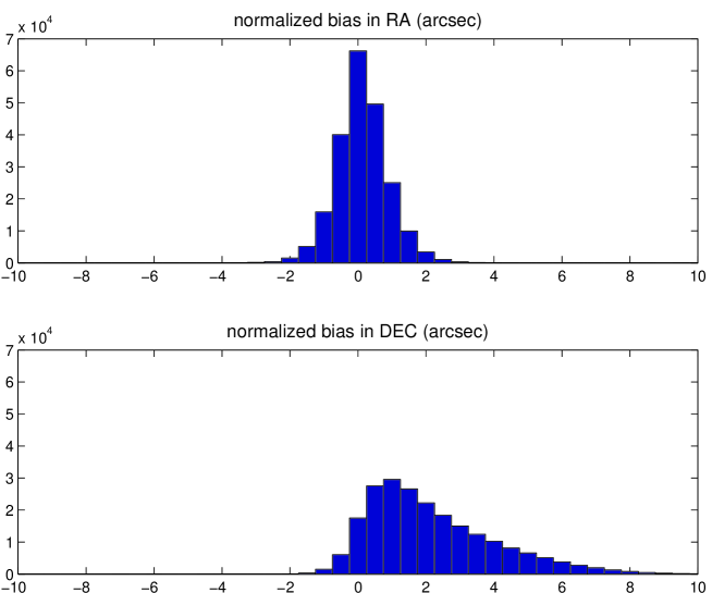
Figure 1 shows that the normalized biases of astrometric residuals for the over-determined orbits of numbered asteroids are strikingly different from a zero-mean Gaussian. The normalized declination bias is qualitatively different from a Gaussian with a mean of $\sim 2.17$ and a standard deviation of $\sim 1.86$. In right ascension the shape is not too different from a normal distribution but with a non-zero mean of $\sim 0.12$ and standard deviation of $\sim 0.77$. The span, curvature and Z-sign have similar non-Gaussian distributions although the declination bias is the worst case. The causes of this behavior and the methods to mitigate their effects are discussed in Section 4.

We need to take into account that the values of the quality metrics are already high even before the attribution when attributing new observations to objects with strongly over-determined orbits. Thus, we cannot use small values of the control parameters because it would generate the paradoxical result that the already computed orbit should be discarded before adding new observations. Even if the new observations improve the orbit determination because they are of better quality and/or extend the observational time span, the systematic error signatures contained in the residuals of the existing orbit are not going to be removed. On the other hand, if we use high values of the controls we may fail to reject some false attributions.

Our solution is to take into account the values of the metrics and the amount they change as a result of the proposed attribution. E.g., for the $RMS$ metrics we accept an attribution only if the increase resulting from the attribution is small (we used $<0.15$ in Table 2). For the other 8 metrics that are based upon astrometric residuals we set an upper limit to the increase in the absolute value (we used $<2$ in Table 2).

3.1 Quality control for new observations

The new observations may have little effect on the statistical properties of the complete set of residuals because the tracklets contain typically only $2$ to $8$ observations while the existing data set typically contains tens or even hundreds of observations, i.e., the residuals may be neither significantly better nor significantly worse. Thus, we need to separately consider the residuals of the attributed observations for which we require the $RMS$, $BIAS$ and $SPAN$ (typical tracklets have no significant curvature and even less Z-sign). For the tests reported in Table 2 we have used the controls $RMS<3,\;|BIAS|<3,\;|SPAN|<3$. These values were chosen empirically based on our experience with both real data and simulations as reported in Milani et al. (2005). Our experience suggests that it is not possible to use theoretically motivated control values from e.g., a $\chi^{2}$ table although they must be of the theoretical order.

The attribution procedure is recursive with tracklets added one by one proceeding in order from the most to least likely as measured by the penalty $K_{4}$. When an attribution has passed all the quality controls and a new orbit has been fit to all the observations including the new tracklet, the new orbit becomes the object’s reference orbit. Then, the other tracklets proposed for attribution from filter 2 are passed to filter 3 and quality control, and so on.

This procedure is robust but we cannot claim that it is perfectly reliable. Due to the stochastic nature of the observational errors any attribution may be wrong; even those that result in the determination of a numbered asteroid orbit, although the probability of this happening has to be very small.

Despite the probability being small, when there are a large number of trials the odds of finding low probability events approaches unity. Our processing attributed a 4-observation PS1 tracklet from the year 2010 to the numbered asteroid (229833) 2009 BQ₂₅; however, the fit to all the available data required discarding 6 observations that were designated 2000 KU₅₁ from the apparition in the year 2000. In this case the only way to decide which attribution to (229833) is correct might be to reexamine the original observations.

4 Data debiasing for historic data

Figure 2: Histogram of normalized astrometric residual biases for all numbered asteroids as in Figure 1 but after removing systematic star catalog errors from all the observations.

The most important source of systematic errors in observations of solar system objects is in the star catalog used for astrometric reduction. Chesley et al. (2010) suggested that the errors could be mitigated by debiasing the astrometric asteroid data with the measured regional catalog biases. The biases can be computed as the average difference in position between the stars in one catalog with respect to another more accurate catalog. Chesley et al. (2010) used the 2MASS star catalog (Skrutskie et al., 2006) as their reference because it is of good accuracy and covers the entire sky with a sufficient number of stars per unit area. The catalog used for the astrometric reduction of each asteroid observation is available for $92.8\%$ of the existing CCD data.

We have implemented an error model consistent with Chesley et al. (2010) by 1) debiasing the observations by subtracting their calculated biases and 2) assigning a per-observation weight that is inversely proportional to the debiased RMS residuals given in Chesley et al. (2010, Table 6) (for the same observatory and the same catalog when known). More precisely, the weight was $1/(2\cdot RMS)$ when known but set to $1/1.5$ arcsec^-1 for data after 1950, for observations performed by photographic techniques, and for CCD observations that do not include star catalog information.

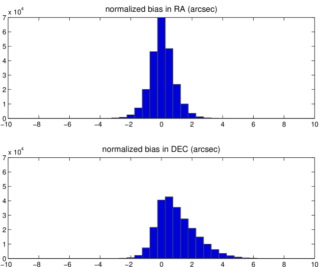
Figure 2 shows that the bias distribution is much less asymmetric after implementation of the error model. The mean of the normalized biases is now $\sim 1.00$ in declination (standard deviation $\sim 1.26$) and $\sim 0.05$ in right ascension (standard deviation $\sim 0.80$). The debiased set of declinations is still biased but improves by a factor $\sim 2$ and the debiased right ascensions has biases at the level of the quality of the best catalogs and is as good as it can currently be. Thus, the observation debiasing and weighting improves the performance of the asymmetric attribution algorithms but highlights that improvements in the star catalogs are still necessary to take advantage of modern high-accuracy asteroid astrometry.

Figure 3: Histograms of declination residuals for PS1 observations of numbered asteroids that were submitted to the MPC through 15 May 2011. Left: with respect to orbits computed with the biased star catalog. Right: after applying debiasing according to Chesley et al. (2010).

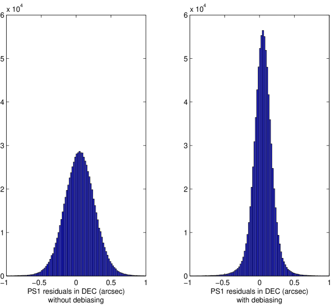
Another way to quantify the improvement of the orbit fit is to measure the residuals with respect to PS1 observations of numbered asteroids. The histograms in Figure 3 show a significant improvement in the declination residuals due to the debiasing; the effect is also significant but less pronounced in right ascension. The debiasing procedure improves the RMS of the residuals from $0.21$ to $0.18$ arcsec in RA and from $0.23$ to $0.16$ arcsec in DEC.

To take advantage of the significant improvements obtained using the Chesley et al. (2010) debiasing the orbit catalogs used for all the tests described in the next two sections have been computed in this way. The technique is now implemented in the free software OrbFit, version 4.2 and later. The debiased orbit catalogs are now available from the AstDyS online service.

5 Tests with PS1 data

The Pan-STARRS prototype telescope, PS1, has a $1.8$ m diameter primary (with an equivalent aperture of $1.55$ m after accounting for the large secondary), a $1.4$ GigaPixel camera, and $7.4$ square degree field of view (Hodapp et al., 2004). The PS1 sky survey is intended to serve multiple scientific goals (e.g., in the solar system Jedicke et al., 2007) for which accurate astrometry is just one of many necessary requirements. The all-sky coverage (from Hawaii) combined with the pixel scale of $0.26$ arcsec makes PS1 potentially capable of excellent astrometry of solar system objects.

The PS1 survey began acquiring engineering data in 2009 and the first tests with our KNOWN_SERVER software that implements the algorithms described herein were run on data taken in June/July of that year. These tests showed that the PS1 astrometry of small solar system objects was extremely good with a standard deviation of $\sim 0.12$ arcsec in right ascension, $\sim 0.13$ arcsec in declination, and a very small bias. (The small bias was due to chance as the observed region of the sky had less star catalog errors than average as discussed below.)

PS1 officially began surveying in May 2010 but the first year’s data set is not fully homogeneous because there were many adjustments to the telescope, camera, survey scheduling, image processing, etc. Nevertheless, the full set of PS1 observations allows us to assess the way the biases change with right ascension. We achieve a more detailed analysis of the PS1 system performance using a smaller but homogeneous dataset.

5.1 Biases in PS1 residuals

We can assess the regional residual systematic errors in the star catalogs using PS1 attributions to numbered asteroids observed through April 2011 that are widely distributed on the celestial sphere. Note that no debiasing is applied for the PS1 astrometry since it already uses the 2MASS catalog (Skrutskie et al., 2006) that was used as the reference catalog in the debiasing procedure (Chesley et al., 2010).

Figure 4: (Top) Right ascensions and (bottom) declinations of PS1 observations attributed to numbered asteroids up to April 2011. The peak in the bin just above $0^{\circ}$ declination is due to the Medium Deep fields (see Section 5.2).

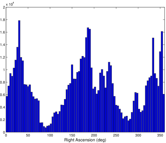
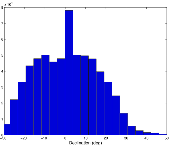
Figure 4 shows the number distribution of the observations as a function of right ascension and declination. The dramatic dips in the RA number distribution at about $105^{\circ}$ and $285^{\circ}$ are where the galactic plane crosses the equator. The PS1 system has a reduced asteroid detection efficiency in the galactic plane because of stellar over-crowding. The distribution is also not uniform in declination but there are enough data for our purposes over most of the range between $-30^{\circ}$ and $+50^{\circ}$.

The right ascension residual bias is strongly dependent on right ascension as shown in the top panel of Figure 5. There is a pronounced maximum of more than $0.1$ arcsec between $110^{\circ}$ and $220^{\circ}$. Note that our first test data set of June/July 2009 was taken between $270^{\circ}$ and $300^{\circ}$ of right ascension where the biases appear to be only around $0.02$ arcsec. On the contrary, there is only a weak dependence of the declination residual biases upon right ascension.

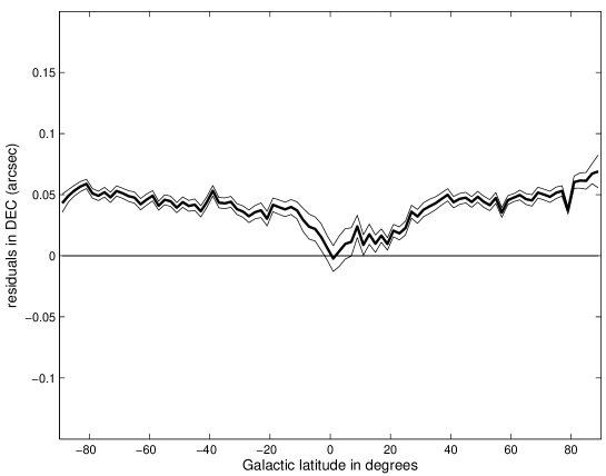
The location of the dips to $\sim 0.00$ arcsec for the declination residual (see bottom panel of Figure 5) match the ranges in RA with limited asteroid statistics as shown in Figure 4 — where the galactic plane crosses the equator. Indeed, Figure 6 highlights the relationship between the biases of the residuals and galactic latitude. It is absolutely clear that where the stellar sky-plane density is high on the galactic equator the residuals disappear.

The dependence of right ascension residual biases upon declination shown in the top panel of Figure 7 has a significant signature but with lower amplitude that never exceeds $0.08$ arcsec. Another significant effect is in the dependence of declination residual bias upon declination as shown in the bottom panel. There is a relatively constant bias residual of $\sim 0.05$ arcsec from about $-30^{\circ}$ to $20^{\circ}$ declination but then a pronounced trend to negative biases as the declination increases to $\sim 50^{\circ}$.

Figure 5: (Top) The middle (thick) curve represents the mean residual in right ascension (multiplied by $\cos\delta$) as a function of right ascension over 2 degree wide bins. The lower and upper curves correspond to $\pm 3$ standard errors on the mean. (Bottom) The same for the declination residual.

Figure 6: (Top) The middle (thick) curve represents the mean residual in right ascension (multiplied by $\cos\delta$) as a function of galactic latitude over 2 degree wide bins. The lower and upper curves correspond to $\pm 3$ standard errors on the mean. (Bottom) The same for the declination residual.

Figure 7: (Top) The middle (thick) curve represents the mean residual in right ascension (multiplied by $\cos\delta$) as a function of declination over 2 degree wide bins. The lower and upper curves correspond to $\pm 3$ standard errors on the mean. (Bottom) The same for the declination residual.

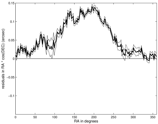
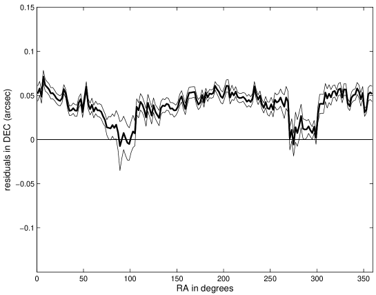
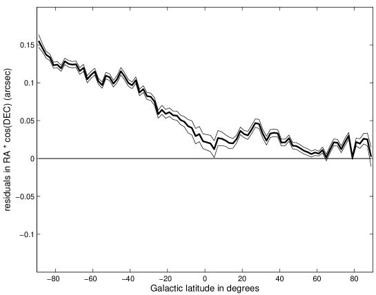
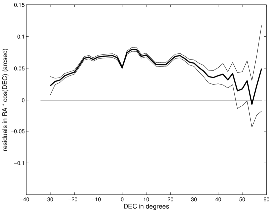
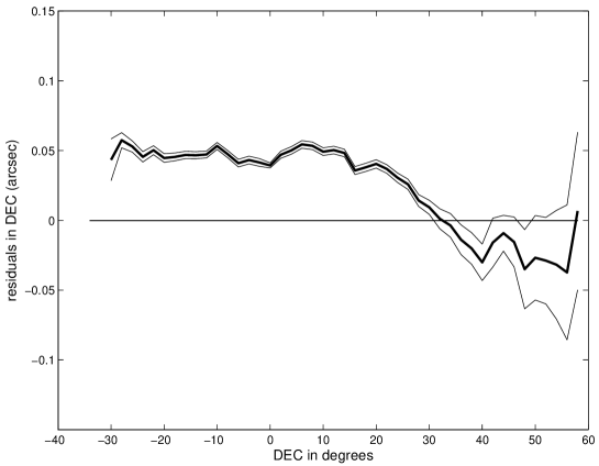
The interpretation of these systematic regional biases would require a dedicated study but we may have uncovered regional biases in the 2MASS star catalog that are significantly smaller than those of other frequently used star catalogs but still relevant when used at the level of accuracy made possible by instruments like PS1. In the medium term we expect this problem would be removed by debiasing the 2MASS catalog in turn with an even better catalog such as the one to be produced by the GAIA mission.

5.2 Standard deviations and correlations in PS1 data

To assess the current PS1 astrometry we have used a homogeneous dataset processed with the same image processing software and astrometric reduction based upon the 2MASS star catalog. As noted above, the Chesley et al. (2010) bias model uses 2MASS as the reference catalog so that the PS1 data do not need debiasing but the historic data from other observatories have been debiased. The attributions to known numbered and multi-opposition objects was performed with the KNOWN_SERVER software with uniform configuration options such as the quality control parameters.

The data belong to lunations 138 and 139 from 3/25/2011 to 4/17/2011 and 4/18/2011 to 5/17/2011 respectively. In each lunation there are tracklets generated in two different types of surveys: 1) the $3\pi$ survey including fields within about $\pm 30^{\circ}$ of the longitude of opposition with four exposures per night and 2) the medium deep survey (MD) with eight exposures per visit at a few specific bore-sights (the same bore-sight might be visited more than once on the same night in different filters). The $3\pi$ opposition fields are typically acquired in the $g_{P1}$, $r_{P1}$ and $i_{P1}$ filters and the MD surveys also use the $z_{P1}$ and $y_{P1}$ filters (see Schlafly et al. (2012) for a detailed description of the PS1 filter system). As mentioned above, the $3\pi$ fields cover a wide area near opposition while the boresite locations of the 5 MD fields used in this work are provided in Table 1.

Table 1: Identifiers, boresite locations and number of reported asteroid observations from the PS1 Medium Deep fields used in this work.

MD Field	RA (deg)	Dec. (deg)	# of obs.
MD03	130.591	44.316	310
MD04	150.000	2.200	5742
MD05	161.916	58.083	41
MD06	185.000	47.116	287
MD07	213.704	53.083	6

Table 2: Mean, RMS and correlation of PS1 right ascension and declination residuals for two lunations and two types of PS1 surveys (mean and RMS in arcsec). The last column is the number of data points in the measurement. The rows in bold are the results after removing the mean (i.e., the standard deviation).

Survey-	right ascension			declination			number
Lunation	Mean	RMS	Corr	Mean	RMS	Corr	resid.
$3\pi$-138	0.115	0.170	0.759	0.078	0.147	0.691	67566
	0.	0.125	0.542	0.	0.125	0.587
$3\pi$-139	0.088	0.154	0.609	0.073	0.149	0.614	44111
	0.	0.127	0.420	0.	0.129	0.480
MD-138	0.035	0.120	0.305	0.014	0.120	0.278	3533
	0.	0.115	0.242	0.	0.119	0.269
MD-139	0.038	0.112	0.332	0.019	0.109	0.340	3047
	0.	0.106	0.257	0.	0.107	0.323

Table 2 gives the basic statistical properties of the residuals for all four data subsets. As expected from the discussion in the previous subsection the bias in both RA and DEC is sensitive to the sky location and the RMS (computed with respect to zero) changes significantly as a consequence. The RMS computed with respect to the mean is less sensitive but it too can change within a range of $0.02$ arcsec.

We also computed the correlations among the residuals of the same coordinate that belong to the same tracklet. They have a large spread that depends on the observed region in the sky and also upon the removal of the constant bias (the mean of the residuals). This is not a surprise since if the data are processed ignoring the presence of a bias then the bias reappears as a correlation. The only unexpected result is the size of this effect with apparent correlations up to $0.76$ in RA and $0.69$ in DEC. In the $3^{\circ}$ wide MD field the overall bias is much less because the target area is subject to low biases in the 2MASS catalog and the removal of the overall mean is almost equivalent to a direction-sensitive debiasing. This results in in-tracklet correlations in the range $0.24$ to $0.32$. These values are a good measure of the intrinsic correlation of data taken over a short time span (such as data from the same tracklet).

These results imply that we are not yet ready to build a PS1 error model that fully accounts for biases and correlations because these two effects cannot yet be neatly separated. To use all the information contained in the precise PS1 observations we would need to first apply a 2MASS catalog (Skrutskie et al., 2006) debiasing, measure the correlation, and then build a PS1-specific error model and explicitly account for the correlations (as was done by Carpino et al. (2003); Baer et al. (2011)). Since this is a significant undertaking it needs to be the subject of our future work and we need to find a method to handle the data in a statistically correct manner.

5.3 Indications for a Pan-STARRS error model

There are two main conclusions to be drawn from the analysis of the PS1 data.

First, the precision of the PS1 astrometry is very good. The random component of the error model for the residuals in both RA and DEC has a standard deviation ranging between $0.106$ and $0.129$ arcsec (see the bold lines in Table 2). This is reasonable taking into account the typical PS1 point spread function (PSF) full-width at half-max of $\sim 1.1$ arcsec, the pixel scale of $\sim 0.26$ arcsec, that asteroids move slightly during the PS1 exposures, and that the vast majority of the reported PS1 asteroid detections have a signal-to-noise ratio (SNR) in the range of 5-10 (i.e., for over-sampled PSFs we expect the astrometric precision to be $\sim FWHM/(2.4\times SNR)$, Neuschaefer and Windhorst (1995)). Only a few professional asteroid observers regularly achieve this astrometric accuracy and of the large surveys only the Sloan Digital Sky Survey appears to have reached such precision. The PS1 advantage is that it achieves this accuracy over the entire sky during a long term survey and will generate a huge volume of data. In 2010 PS1 was the fifth largest contributor of numbered asteroid observations to the MPC with $548,518$ (in the first 11 months of 2011 it was fourth with $935,001$).

Second, the accuracy of the PS1 astrometry is limited by the presence of systematic errors in the reference star catalog. Although 2MASS (Skrutskie et al., 2006) is the best possible choice for a star catalog it still contains systematic effects at up to the level of $0.1$ arcsec that are easily detectable with the modern generation of sky surveys. As a consequence, it is not yet possible to fully capitalize on the astrometric precision available from surveys like PS1. The problem could be solved either with new and improved star catalogs (e.g., the ones expected from the GAIA mission) or by building a survey-specific PS1 star catalog that is referenced to a catalog with smaller regional biases such as Tycho-2 or Hipparcos. In addition to the position-dependent biases there is also an intrinsic correlation among the observations belonging to the same tracklet that we are not able to model accurately at this time.

To ensure that the PS1 observations yield the best possible nominal solutions and reliable covariance estimates the PS1 residuals must be weighted in a manner that accounts for systematic errors and their correlations. That is, if we use a model that ignores biases and correlations the confidence region of the observations of the same tracklet needs to be a sphere containing the ellipsoid representing the confidence region of the debiased and correlated model. If we assume the correlated covariance matrix of the RAs of the tracklets with $m$ observations has variances $\sigma^{2}$ on the diagonal and all correlations are equal to $r$ (i.e., the covariances are all $r\,\sigma^{2}$) then the largest eigenvalue is $(1+(m-1)\,r)\cdot\sigma^{2}$ (Milani and Gronchi, 2010, Section 5.8). With $m=4$, $r=0.759$, $\sigma=0.170$ the maximum eigenvalue is $0.308^{2}$. Thus, the worst case from Table 2 requires a weight of $1/0.308$ arcsec^-1. Indeed, AstDyS uses a weight of $1/0.3$ to process the PS1 data — the highest weight for any asteroid survey. Some asteroid programs with either special instruments/methods or very labor intensive reduction procedures do have higher weights.

We are not claiming that this weighting scheme is the best or only solution for handling high precision data from modern surveys — only that it is a prudent way to use the PS1 data while waiting for a more sophisticated error model that could be obtained by a better bias removal and by an explicit correlation model.

6 Accuracy and efficiency

The purpose of this section is to measure the accuracy and the efficiency of our asymmetric attribution procedure. Accuracy is the fraction of correct attributions among those proposed by our method while efficiency is the fraction of possible attributions that were found.

6.1 Accuracy test

It is very difficult to measure accuracy with real data because it is impossible to know the ground truth (i.e., which attributions are true/false) while measuring accuracy with simulated data would be less convincing because it is difficult to simulate all possible causes of false data (at the single detection, tracklet, and attribution level). In any event, false data tend to generate tracklets with randomly oriented angular velocity that are less likely to be attributed to a real asteroid orbit. We therefore consider an attribution test with real tracklets and real objects to be more valuable at least for the same number of tracklets under consideration.

Our solution has been to use the fact that our dataset of proposed attributions can be split in two disjoint subsets: numbered and multi-apparition asteroids. The set of all attributions to numbered objects is robust and contains only a very small fraction of false attributions. If a tracklet has a successful attribution to a numbered asteroid then it cannot be attributed to a different asteroid. Thus any tracklet that is already attributed to a numbered asteroid would almost certainly be a false attribution if it could also be attributed to a multi-apparition asteroid.

In our test we used the set of $13,729$ tracklets attributed to numbered asteroids in lunation 139 of the PS1 $3\pi$ survey and attempted to find attributions to a list of $140,225$ multi-apparition orbits using our algorithm for the asymmetric case. The multi-apparition orbits provide much less accurate ephemerides and finding an observation inside the confidence ellipse of one of the many tested orbits is not a rare event. The first filter provided $44,675$ candidate attributions, the second filter reduced the number to 8, and the third yielded 3 tracklets incorrectly attributable to two asteroids: 2010 GU₁₀₄ (2 tracklets) and 2010 GK₂ (1 tracklet).

For comparison, our algorithm attributed $3,619$ tracklets to $2,950$ multi-apparition asteroids in the same lunation after removing all the tracklets that were already attributed to numbered asteroids. Thus, the false attribution rate can be estimated at either $3/3,619$ or $2/2,950$ which is $<1/1,000$ per lunation per observable object. This result is statistically good but cannot be ignored because such false attributions would introduce permanent ‘damage’ in the orbit database.

The false attribution rate can be reduced to zero through additional controls. The two asteroids 2010 GU₁₀₄ and 2010 GK₂ for which false attributions were found have a historical set of observations that only weakly constrain the orbit: two apparitions widely spaced in time (1999–2010 and 2001–2010 respectively) and not many observations (16 and 18 respectively). Thus, the $1\,\sigma$ ephemeris confidence ellipses at the time of the incorrect attribution have major semiaxes of about $47$ and $81$ arcmin, respectively. This explains why it was possible to find a false attribution passing the quality controls in a sample of $>13,700$ tracklets. Moreover, in the first case the two attributed tracklets were from a single night and in the second there was only one tracklet. Thus, another filter should not accept single-night attributions to objects that have been observed in only two previous apparitions. As a matter of fact, the Minor Planet Center has enforced this rule for a long time and we acknowledge that this rule is a meaningful caution to avoid contamination of the orbits database by spurious attributions such as the ones found in our test.

6.2 Efficiency test

Determining the efficiency of our attribution method suffers from the same concerns addressed above regarding the use of real or synthetic data. Once again, we decided to rely on real data and used the AstDyS catalog of numbered and multi-apparition asteroids to identify a set of asteroids whose ephemeris definitely places them in each field of view. The PS1 limiting magnitude is fainter than most known asteroids when they are at opposition so we used objects identified in one night of morning sweet spot observations (looking eastwards before sunrise at solar elongations between $60^{\circ}$ and $90^{\circ}$ in the $w$ filter). Main belt asteroids are fainter in the sweet spots than at opposition due to distance and phase angle effects so that their range in apparent magnitude is better suited to determining the PS1 sensitivity as a function of the object’s brightness.

Then we ran KNOWN_SERVER using the same catalog of orbits and all the observed tracklets in the same fields to identify objects in the list of those which could have been observed because they were in the field of view of the PS1 sensor. The efficiency is simply the fraction of observable objects that were actually detected. If the false attribution rate is $<1/1,000$ as discussed in the previous subsection the statistics of the successful attributions will not be significantly contaminated.

Figure 8 shows that the attribution efficiency as a function of predicted apparent V magnitude has a sharp decline at the limiting magnitude of $\sim 21$ (where the efficiency drops to half the peak value). The peak efficiency of $\epsilon_{max}=0.78\pm 0.04$ occurs at $V\gtrsim 19$ but decreases by less than a standard deviation in the brightest bin near $V\sim 18$ to $0.74\pm 0.04$. Note that the well known offset of a few tenths of a magnitude between predicted and actual asteroid $V$ magnitudes (Jurić et al., 2002) is unimportant — all we care about here is the peak efficiency independent of magnitude.

Figure 8: Tracklet attribution efficiency to well known asteroid orbits as a function of predicted apparent V magnitude from one night of the PS1 survey. Each data point represents 150 observable objects. The horizontal bars indicate the range of values within the bin and the vertical bars represent one standard deviation of the estimated efficiency in the bin.

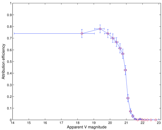
The problem in interpreting these results is that they measure several different contributions to the efficiency including the fill factor ($f$, the fraction of the focal plane covered by active sensing pixels), the detector sensitivity ($\epsilon_{D}$), the efficiency of the image processing pipeline (IPP) in detecting moving objects ($\epsilon_{IPP}$), the Moving Object Processing System’s (MOPS,  Kubica et al., 2007) efficiency at linking detections into tracklets ($\epsilon_{MOPS}$), and the efficiency of the attribution algorithm ($\epsilon_{attrib}$). Disentangling each effect as a function of $V$ is difficult but unnecessary for our purposes. Instead, we know that the generic efficiency $\epsilon_{x}\geq\epsilon_{max}$ and attempt to establish a minimum value of $\epsilon_{attrib}$.

The PS1 camera consists of 60 orthogonal transfer array (OTA) CCDs arranged in an $8\times 8$ array (the four corners do not have CCDs) and each OTA contains an on-chip $8\times 8$ mosaic of ‘cells’. The camera fill factor includes the physical gaps between OTAs, smaller gaps between cells on a single OTA, area lost to defective cells and bad pixels, and the overlap between the sensor and the Field Of View (FOV) of the optical system. There are additional losses of the order of $1\%$ specific to individual exposures due to a ‘dynamic mask’ applied to remove bright diffraction spikes and internal reflections.

The PS1 image processing team produces periodic analysis of sensor fill factor as the camera tuning improves. The most recent study (May 2010) yields $f=0.79$ due to a $7.0\%$ loss due to inter-OTA gaps, a $4.3\%$ loss due to inter-cell gaps, and $9.7\%$ mask fraction in the UN-vignetted 3.0-degree FOV. For our KNOWN_SERVER efficiency study we only consider asteroids that should appear in the 3.0-degree FOV so $f=0.79$ is applicable.

The fill factor estimate implies that the peak efficiency (at magnitudes between 19 and 20) leaves little room for losses due to the IPP, MOPS, and attribution software. Each of the processing steps has a minimum efficiency of $0.98^{+0.02}_{-0.05}$. I.e., the overall efficiency is dominated by the fill factor and the efficiency of the other steps including attribution is consistent with 100%. The apparent drop in the efficiency for brighter apparent magnitudes is not significant. It might indicate some problems in the image processing and accurate astrometric reduction of bright detections. The PS1 CCDs saturate at about $w=15.9$ and the $w$-filter is used for sweet spot observations.

7 Conclusions and future work

We proposed a new procedure to identify known asteroids among the new observations from a survey. This procedure solves the problems due to the asymmetry in quantity and quality between the data and historic observations.

We tested the procedure with real data from the Pan-STARRS PS1 survey and assessed the performance of our algorithms and the astrometric accuracy of the survey data. The main results are the following.

First, the new algorithms are accurate and efficient. For multi-apparition asteroids the false attribution fraction is less than $1/1,000$ and even those can be eliminated by following the MPC’s good practice of requiring two nights of data for a recovery at a new apparition. The algorithm’s attribution efficiency is high and consistent with 100% but cannot really be measured because it is entangled with other efficiency losses such as the fill factor.

Second, the PS1 data have significantly lower astrometric error than other asteroid surveys. This error can be identified only after removing the biases due to systematic errors in the star catalogs. Indeed, we arrived at the conclusion that even the 2MASS star catalog contains enough biases to affect the PS1 error model. It is likely that the use of other catalogs, or at least debiasing with respect to them, would further improve the PS1 error model; e.g., Tycho-2 could be used now and the GAIA catalog in the future.

Third, we consider that the PS1 data can be included in the fit for asteroid orbits with weights corresponding to $1/0.3$ arcsec^-1 that implicitly account for the effects of correlations. A model with debiasing of the 2MASS astrometry and explicitly taking into account the correlations could allow a further improvement in the diagonal elements of the weighting matrix by another factor $2\sim 3$.

7.1 Future work

Apart from the improvements mentioned above there are three areas where there is room for future developments.

The first is in the use of KNOWN_SERVER, or similar algorithms and software, as a filter to remove observations of known objects from a new set of data to leave subset with a larger fraction of potential new discoveries. Although we think that this principle is valid we have not yet been able to test the idea on real data. For the removal of the known objects to be a significant contribution in decreasing the false identification rate, the false tracklet rate must be below some threshold and the number of known objects must be large compared to the number of unknown objects at the system’s limiting magnitude. For the current PS1 data the false discoveries due to spurious detections (that form false tracklets) are more important than the false discoveries due to incorrect linking of true tracklets.

The second is the possibility of using KNOWN_SERVER as an alarm to detect unusual phenomena in well known asteroids. The most interesting cases could be the Main Belt Comets (MBC,  Hsieh and Jewitt, 2006).

As an example, the numbered asteroid (300163) was found to be a MBC on the basis of PS1 observations that showed an image wider than the PSF of nearby stars (Hergenrother, 2011). However, the standard KNOWN_SERVER output automatically flags these observations as very unusual in at least 3 different ways. Two of the strange flags are astrometric in nature: $BIAS_{\alpha}=4.01$, corresponding to a systematic shift by $0.85$ arcsec backward (with respect to orbital motion), and $BIAS_{\delta}=2.11$, corresponding to a shift by $0.44$ arcsec North. These could be interpreted as an effect of displacement of the center of light with respect to the center of mass, and/or as an effect of non-gravitational perturbations. The other strange flag was that the observation’s apparent magnitudes were on average brighter than the predicted ones by about $1.05$ which is also likely a consequence of the outburst.

The problem is to define a filter selecting anomalous behaviors such as the one above as an indication of possible orbital, luminosity and/or image shape changes. The main challenge is to design such a filter with a low false positive rate that allows for dedicated follow up of the MBC candidates.

The third is the possibility of improving the quality of other existing large datasets (such as those generated by other sky surveys or even the MPC asteroid astrometry database) by either detecting missing attribution or proposing deletion of dubious ones. This work would require the collaboration of the data providers for their insight on the datasets’ problems.

References

- Baer et al. (2011) Baer, J., Chesley, S. R., Milani, A. 2011. Development of an observational error model. Icarus 212, 438-447.
- Chesley et al. (2010) Chesley, S. R., Baer, J., Monet, D. G. 2010. Treatment of star catalog biases in asteroid astrometric observations. Icarus 210, 158-181.
- Carpino et al. (2003) Carpino, M., Milani, A., Chesley, S. R. 2003. Error statistics of asteroid optical astrometric observations. Icarus 166, 248-270.
- Granvik and Muinonen (2008) Granvik, M., Muinonen, K. 2008. Asteroid identification over apparitions. Icarus 198, 130-137.
- Hsieh and Jewitt (2006) Hsieh, H. H., Jewitt, D. 2006. A Population of Comets in the Main Asteroid Belt. Science 312, 561-563.
- Hergenrother (2011) Hergenrother, C. W. 2011, Central Bureau Electronic Telegrams, 2920, 2
- Hodapp et al. (2004) Hodapp, K. W. et al. 2004. Design of the Pan-STARRS telescopes. Astronomische Nachrichten 325, 636-642.
- Jedicke et al. (2007) Jedicke, R., Magnier, E. A., Kaiser, N., Chambers, K. C. 2007. The next decade of Solar System discovery with Pan-STARRS. IAU Symposium 236, 341-352.
- Jurić et al. (2002) Jurić, M., and 15 colleagues 2002. Comparison of Positions and Magnitudes of Asteroids Observed in the Sloan Digital Sky Survey with Those Predicted for Known Asteroids. The Astronomical Journal 124, 1776-1787.
- Kubica et al. (2007) Kubica, J. et al. 2007. Efficient intra- and inter-night linking of asteroid detections using kd-trees. Icarus 189, 151-168.
- Marsden (1985) Marsden, B. G. 1985. Initial orbit determination - The pragmatist’s point of view. The Astronomical Journal 90, 1541-1547.
- Milani (1999) Milani, A. 1999. The Asteroid Identification Problem. I. Recovery of Lost Asteroids. Icarus 137, 269-292.
- Milani et al. (2001) Milani, A., Sansaturio, M. E., Chesley, S. R. 2001. The Asteroid Identification Problem IV: Attributions. Icarus 151, 150-159.
- Milani et al. (2005) Milani, A., Gronchi, G. F., Knežević, Z., Sansaturio, M. E., Arratia, O. 2005. Orbit determination with very short arcs. II. Identifications. Icarus 179, 350-374.
- Milani et al. (2008) Milani, A., Gronchi, G. F., Farnocchia, D., Knežević, Z., Jedicke, R., Denneau, L., Pierfederici, F. 2008. Topocentric orbit determination: Algorithms for the next generation surveys. Icarus 195, 474-492.
- Milani and Gronchi (2010) Milani, A., Gronchi, G. F. 2010. Theory of Orbital Determination. Theory of Orbital Determination, by Andrea Milani and Giovanni F. Gronchi. ISBN 978-0-521-87389-5. Published by Cambridge University Press, Cambridge, UK, 2010.
- Neuschaefer and Windhorst (1995) Neuschaefer, L. W., Windhorst, R. A. 1995. Observation and reduction methods of deep Palomar 200 inch 4-Shooter mosaics. The Astrophysical Journal Supplement Series 96, 371-399.
- Sansaturio and Arratia (2011) Sansaturio, M. E., Arratia, O. 2011. Mining knowledge in One Night Stands data sets. Monthly Notices of the Royal Astronomical Society 1935.
- Schlafly et al. (2012) Schlafly, E. F., D. P. Finkbeiner, D. P., Juri´c, M., Magnier, E. A. 2012. Photometric calibration of the first 1.5 years of the PAN-STARRS1 survey (submitted).
- Skrutskie et al. (2006) Skrutskie, M. F. et al. 2006. The Two Micron All Sky Survey (2MASS). The Astronomical Journal 131, 1163-1183.