Nonlinear reaction with fractional dynamics

Abstract

In this paper we consider a system of three fractional differential equations describing a nonlinear reaction. Our analysis includes both analytical technique and numerical simulation. This allows us to control the efficiency of the numerical method. We combine the numerical approximation of fractional integral with finding zeros of a function of one variable. The variable gives a desired solution. The solution has a peak. Its position in time depends on the order of fractional derivative. The two other solutions of this system have a completely monotonic character.

1 Introduction

The dynamical systems with fractional dynamics are adequate for the description of various physical phenomena in viscoelasticity, diffusion processes, dielectric relaxation, etc [1, 2, 3, 4]. However, now the analysis of nonlinear differential equations with fractional derivatives is in early development. The point is that on the one hand the derivation of such equations from some initial principles is in the making. On the other hand the numerical simulation of fractional differential equations are enough expensive [5]. In the present state of affairs it may follow a formal way by changing the derivatives of integer order in the well-known nonlinear equations on the derivative of an arbitrary order. This means a search to the touch together with overcoming the difficulties of numerical analysis. So that was at the beginning of fractional calculus. But there exists an alternative way. The other approach may be based on the recent success in the study of linear fractional differential equations. In particular, the linear fractional equations have been well investigated analytically in detail [6, 7, 8]. Moreover, the fractional oscillator and the fractional relaxation have an clear physical interpretation [9, 10]. Some nonlinear models turn out to be very close to linear ones in a sense. This permits one to combine analytical computations with simple numerical simulations. The aim of this work is to present one of such nonlinear systems under fractional dynamics.

The plan of the paper is as follows. Section 2 is devoted to a derivation of the nonlinear reaction obeying a stochastic time arrow. The arrow leads to a system of fractional differential equations that describe the process evolution. One of the equations can be resolved by analytical methods. The sum of the two others has also an clear analytical form. The feature analysis is represented in Section 3. Nevertheless, the system of the equations upon the whole is nonlinear. Therefore, the next step is directed to numerical simulations of those equations what cannot be resolved analytically. We rewrite them in the integral form and apply a recursive procedure of numerical fractional integration. It should be observed here that the results obtained in Section 3 proves to be useful for Section 4. We sum up and discuss the outcome in Section 5.

2 Theoretical model

The nonlinear processes play an important role in the kinetics of chemical reactions [11]. The typical example is a reaction in the gas that consists of atoms of two grades ($A$ and $B$). The reaction $A+B=AB$ creates two-atom molecules. In the same time it is not impossible an inverse process, dissociation $AB=A+B$. The dynamical system can be described by differential equations in the nonlinear form.

One of similar nonlinear reactions is mentioned in [12]. Its temporal evolution is written as

$$\frac{dy_{1}}{dt} = -y_{1}\,,$$

$$\frac{dy_{2}}{dt} = y_{1}-y^{2}_{2}\,,$$ (1)

$$\frac{dy_{3}}{dt} = y^{2}_{2}\,,$$

with the initial condition $N_{1}/N=y_{1}(0)=1$, $N_{2}/N=y_{2}(0)=0$, $N_{3}/N=y_{3}(0)=0$, where $N$ is the common number of atoms, and $N_{1}$, $N_{2}$, $N_{3}$ the number of molecules of three types arising from the chemical reaction of the atoms. The equation for $y_{1}(t)$ is linear and is independent from $y_{2}(t)$ and $y_{3}(t)$. Using the stochastic time arrow described in [9], the equation is easily generalized in the fractional form.

The stochastic time arrow characterizes an interaction of a physical system with environmental degrees of freedom. Then the time variable becomes a sum of random temporal non-negative intervals $T_{i}$. They are independent identically distributed variables belonging to a Lévy-stable distribution. Their sum gives asymptotically a stable distribution with the index $0<\alpha\leq 1$. Following the arguments of [9, 13], a new time clock is defined as a continuous limit of the discrete counting process $N_{t}=\max\{n\in{\bf N}:\sum_{i=1}^{n}T_{i}\leq t\}$, where ${\bf N}$ is the set of natural numbers. The time clock is the hitting time process $S(t)$. Its basic properties has been represented in [13, 14]. The probability density of the process $S(t)$ is written in the form

$$p^{S}(t,\tau)=\frac{1}{2\pi i}\int_{Br}e^{ut-\tau u^{\alpha}}\,u^{\alpha-1}\,du\,,$$ (2)

where $Br$ denotes the Bromwich path. This probability density has a clear physical sense. It defines the probability to be at the internal time $\tau$ on the real time $t$ (see details in [9]).

Let us make use of the general kinetic equation

$$\frac{dp(t)}{dt}=\hat{\bf W}p(t)\,,$$ (3)

where $p(t)$ defines the transition probability (or the concentration of a substance) in a system, $\hat{\bf W}$ is the transition operator between the system states. In a general case the operator $\hat{\bf W}$ may be even nonlinear. Provided that it is independent on time explicitly. Now we determine a new process with the probability

$$p_{\alpha}(t)=\int_{0}^{\infty}p^{S}(t,\tau)\,p(\tau)\,d\tau\,.$$ (4)

It is that the function $p^{S}(t,\tau)$ characterizes the stochastic time arrow. The Laplace transform of the probabilities $p_{\alpha}(t)$ and $p(t)$ gives the relation $\tilde{p}_{\alpha}(s)=s^{\alpha-1}\tilde{p}(s^{\alpha})$ with $0<\alpha\leq 1$, and the Laplace image of $x(t)$ is written as

$$\tilde{x}(s)=\int_{0}^{\infty}e^{-st}x(t)\,dt\,.$$

By the simple algebraic computations we have

$$\hat{\bf W}\tilde{p}_{\alpha}(s)=s^{\alpha}\tilde{p}_{\alpha}(s)-p(0)s^{\alpha-1}\,.$$

After the Laplace inverse transform the fractional representation of Eq.(3) takes the form

$$p_{\alpha}(t)=p(0)+\frac{1}{\Gamma(\alpha)}\int_{0}^{t}d\tau\,(t-\tau)^{\alpha-1}\,\hat{\bf W}p_{\alpha}(t)\,.$$ (5)

Although Eq.(5) is integral, it can be expressed in terms of fractional derivative [9, 13, 14]. This approach permits one to generalize Eqs.(1) in that way too. For more details, see the next section.

3 Analytical calculations

Consider the following nonlinear system described by fractional differential equations [15]

$$\frac{d^{\alpha}y_{1}}{dt^{\alpha}} = -y_{1}\,,$$

$$\frac{d^{\alpha}y_{2}}{dt^{\alpha}} = y_{1}-y^{2}_{2}\,,$$ (6)

$$\frac{d^{\alpha}y_{3}}{dt^{\alpha}} = y^{2}_{2}\,,$$

under the initial condition

$$y_{1}(0)=1,\quad y_{2}(0)=0,\quad y_{3}(0)=0,$$

where $0<\alpha\leq 1$. Here the fractional operator $d^{\alpha}/dt^{\alpha}$ is supposed in the sense of Caputo [16]:

$$\frac{d^{\alpha}x(t)}{dt^{\alpha}}=\frac{1}{\Gamma(n-\alpha)}\int^{t}_{0}\frac{x^{(n)}(\tau)}{(t-\tau)^{\alpha+1-n}}\,d\tau,\quad n-1<\alpha<n,$$

where $x^{(n)}(t)$ means the $n$-derivative of $x(t)$. To sum up Eqs.(6), we get

$$\frac{d^{\alpha}(y_{1}+y_{2}+y_{3})}{dt^{\alpha}}=0\quad\Rightarrow\quad y_{1}+y_{2}+y_{3}=1\,.$$

The system analysis shows above all that the first equation for $y_{1}$ is linear. It may be integrated analytically, namely $y_{1}(t)=E_{\alpha}(-t^{\alpha})$. The variable $y_{1}$ is expressed in term of the one-parameter Mittag-Leffler function $E_{\alpha}(z)$. Thus, the value $y_{1}$ becomes vanishingly small with $t\to\infty$ as $t^{-\,\alpha}/\Gamma(1-\alpha)$. On the other hand, from the second and third equations it follows that the sum of $y_{2}$ and $y_{3}$ gives

$$\frac{d^{\alpha}(y_{2}+y_{3})}{dt^{\alpha}}=y_{1}\,.$$

This means that the definition of $y_{1}$ allows one to establish the functional dependence between $y_{2}$ and $y_{3}$. Therefore, the sum takes the form

$$y_{2}+y_{3}=1-E_{\alpha}(-t^{\alpha})\,.$$

This result tends to one as $t\to\infty$.

We find it useful to define the identity

$$E_{\alpha,1}(-t^{\alpha})+t^{\alpha}E_{\alpha,\,1+\alpha}(-t^{\alpha})=1\,,$$

where $E_{\alpha,\,\beta}(z)=\sum_{n=0}^{\infty}z^{n}/\Gamma(\alpha n+\beta)$ is the two-parameter Mittag-Leffler function, and $E_{\alpha}(z)$ is a particular case of $E_{\alpha,\,\beta}(z)$, namely $E_{\alpha,1}(z)$. The Laplace image of $t^{\alpha}E_{\alpha,1+\alpha}(-t^{\alpha})$ is written as

$$\int_{0}^{\infty}e^{-st}\,t^{\alpha}E_{\alpha,1+\alpha}(-t^{\alpha})\,dt=\frac{1}{s}\,\frac{1}{(1+s^{\alpha})}\,,$$

while

$$\int_{0}^{\infty}e^{-st}\,E_{\alpha,\,1}(-t^{\alpha})\,dt=\frac{s^{\alpha-1}}{(1+s^{\alpha})}\,.$$

The sum of these images reduces to $1/s$.

In the upshot it still remains to find the variable $y_{2}$. The value satisfies a nonlinear fractional differential equation with the right-hand term. In other words this equation is inhomogeneous:

$$\frac{d^{\alpha}y_{2}}{dt^{\alpha}}+y^{2}_{2}=E_{\alpha}(-t^{\alpha})\,.$$ (7)

Its form is such that for the final conclusion it is necessary to provide a numerical simulation. Nevertheless, our analytical analysis will not be full without asymptotic estimations as applied to $y_{2}$. If $\alpha$ is equal to one, we can neglect the right-hand term because of its exponential decay. The value $y_{2}(t)$ behaves algebraic for $t\gg 1$. If the index $\alpha$ is otherwise ($0<\alpha<1$), the right-hand term of Eq.(7) is the one-parameter Mittag-Leffler function having an algebraic asymptotic form. What term in Eq.(7) gives a significant contribution in a given case? The feature will be established by a numerical simulation more clearly. The variable $y_{2}(t)$ becomes vanishingly small, when $t$ tends to infinity.

Figure 1: Nonlinear reaction with ordinary time evolution (1) .

Moreover, the Adomain’s composition method assumes a series solution for $y_{2}$ [15]. The first three terms of this series are given by

$$y_{2}(t)=\frac{t^{\alpha}}{\Gamma(1+\alpha)}-\frac{t^{2\alpha}}{\Gamma(1+2\alpha)}+\left(1-\frac{\Gamma(2\alpha+1)}{\Gamma^{2}(\alpha+1)}\right)\frac{t^{3\alpha}}{\Gamma(3\alpha+1)}\,\dots\,.$$ (8)

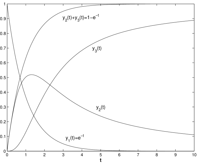
They indicate the presence of a maximum. However, the determination of its properties (position and value) is not enough reliable for the composition method. The point is that the Taylor series converges only for $0<t<1$, but the maximum is the case for $t>1$. Thus the estimation (8) for the maximum will not be exact. This can be easy to verify numerically for $\alpha=1$, using the usual methods (for example, the Runge-Kutta technique or something like that). In this case, the system (6) consists of first-order differential equations. Their numerical solutions are represented in Fig. 1 .

4 Numerical approximation

To solve the nonlinear fractional differential equation, the principal approach is to use a numerical approximation of fractional integral. Its advantage is due to the fact that the kernel of this integral is regular for $\alpha>1$, and weekly singular for $0<\alpha<1$, hence integrable (at least in the improper sense) for any index $\alpha>0$. In contrast, the kernel of fractional derivative is not integrable, and it requires special regularization methods restricting possibilities of the numerical simulation [17].

Let $\{t_{n}=nh:n=0,1,2,\dots,N\}$ be a partition of the interval $[0\ \ T]$ into a grid, where $h=T/N$. According to [17], the fractional integral of the value $y$ is computed as

$$J^{\alpha}y_{N}=\frac{h^{\alpha}}{\Gamma(2+\alpha)}\sum_{n=0}^{N}c_{n}^{(N)}y_{n}\,,$$ (9)

where the quadrature weights are derived from a product trapezoidal rule to the following:

$$c_{n}^{(N)}=\cases{(1+\alpha)N^{\alpha}-N^{\alpha+1}+(N-1)^{\alpha+1}\,,&if $n=0$;\cr 1\,,&if $n=N$;\cr(N-n+1)^{\alpha+1}-2(N-n)^{\alpha+1}+&\cr+(N-n-1)^{\alpha+1}\,,&if $0<n<N-1$.\cr}$$

The error of this algorithm is of order $O(h^{2})$. The accuracy can be improved by the Richardson extrapolation procedure [17].

Figure 2: Fractional one-half-order integral of the exponential function, $J^{1/2}\exp(-t)$, obtained from Eq.(10) (line) and by means of Eq.(9) (circles).

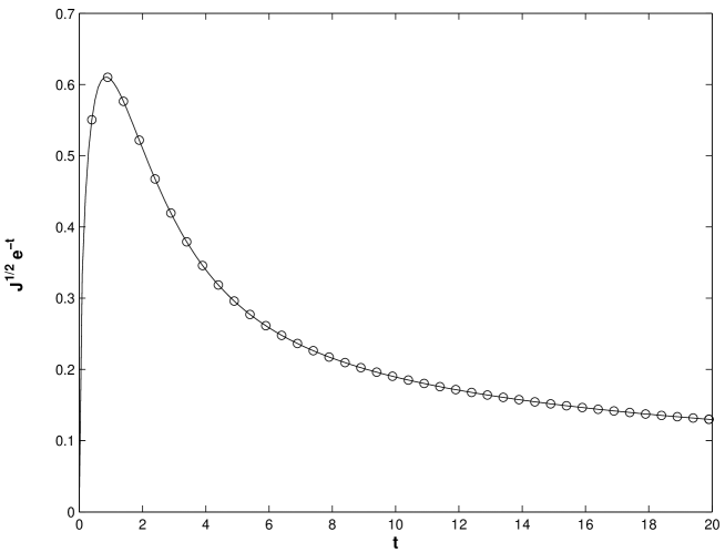
As an example to this algorithm, we suggest to consider the fractional one-half-order integral of the exponential function. The integral has an analytical representation:

$$J^{1/2}\exp(-t) = \frac{1}{\Gamma(1/2)}\int_{0}^{t}(t-\tau)^{-1/2}\,e^{-\,\tau}\,d\tau=$$ (10)

$$= \frac{1}{\sqrt{\pi t}}\int_{0}^{\infty}e^{-\,\tau^{2}/(4t)}\,\sin\tau\,d\tau=e^{-\,t}\mathrm{erfi}(\sqrt{t})\,,$$

where $\mathrm{erfi}(x)=\frac{2}{\sqrt{\pi}}\int_{0}^{x}\exp(y^{2})\,dy$ is the imaginary error function. The transcendental function is expanded into a Taylor series about $x$:

$$\mathrm{erfi}(x)=\frac{2}{\sqrt{\pi}}\sum_{m=0}^{\infty}\frac{x^{2m+1}}{(2m+1)m!}\,.$$

The expansion allows one to compare $J^{1/2}\exp(-t)$ in the analytical form (10) with the numerical simulation result of the fractional integral by means of the above-mentioned algorithm (9) (see Fig. 2).

Figure 3: Nonlinear reaction with time evolution under fractional derivative with the index $\alpha=0.8$ .

Next we transform Eq.(7) into the integral form:

$$J^{\alpha}\frac{d^{\alpha}y_{2}(t)}{dt^{\alpha}}+J^{\alpha}y^{2}_{2}(t)=y_{2}(0)+y_{2}(t)+J^{\alpha}y^{2}_{2}(t)=1-E_{\alpha}(-t^{\alpha})\,.$$ (11)

It is useful to remark the following property: $0\leq y_{2}(t)+J^{\alpha}y^{2}_{2}(t)\leq 1$. As $J^{\alpha}y^{2}_{2}(t)\geq 0$, it is easy to find $0\leq y_{2}(t)\leq 1$. The upper limit of $y_{2}(t)$ is too strong. As will be shown below, $y_{2}(t)$ is less than one. The positivity property of $y_{2}(t)$ at any time is very important. The same exists also for $y_{1}(t)$ and $y_{3}(t)$. Both functions $y_{1}(t)$ and $y_{3}(t)$ are completely monotonic, but $y_{2}(t)$ is not. The latter has a maximum.

Applying the approximation (9), Eq.(11) is written as

$$y_{2}(Nh)+\frac{h^{\alpha}}{\Gamma(2+\alpha)}\sum_{n=0}^{N}c_{n}^{(N)}y_{2}^{2}(nh)=1-E_{\alpha}(-N^{\alpha}h^{\alpha})\,.$$

The expression takes the form of an ordinary quadratic equation:

$$\frac{h^{\alpha}}{\Gamma(2+\alpha)}\,y^{2}_{2}(Nh) + y_{2}(Nh)+\frac{h^{\alpha}}{\Gamma(2+\alpha)}\sum_{n=0}^{N-1}c_{n}^{(N)}y^{2}_{2}(nh)-$$ (12)

$$- 1+E_{\alpha}(-N^{\alpha}h^{\alpha})=0\,.$$

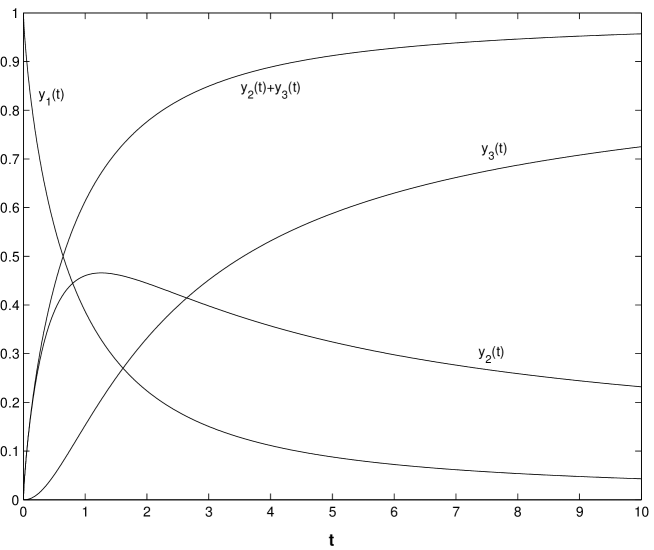
Then the recursive procedure is obtained in an elementary manner. The numerical scheme permits one to calculate $y_{2}(nh)$ from $y_{2}((n-1)h)$ to solve the quadratic equation. Each subsequent value of $y_{2}$ depends on previous ones, because the fractional integration exhibits a long-term memory loss. For computing the one-parameter Mittag-Leffler function $E_{\alpha}(-t^{\alpha})$ we use a numerical scheme listed in Algorithm 4 [17] that is reproduced with minor corrections from [18]. The quadratic equation (12) has two solutions. One of them is positive, and another is negative. We select the non-negative solution in the force of the above analysis to the analytical properties of $y_{2}(t)$. The temporal evolution of this system for $\alpha=0.8$ is shown in Fig. 3. Formally, the system behavior for $0<\alpha<1$ is like to the system one for $\alpha=1$: the variable $y_{1}(t)$ monotonically tends to zero, the variable $y_{3}(t)$ to one, and the variable $y_{2}(t)$ possesses one maximum after which it decays to zero. But there are differences that we discuss in the next section.

Figure 4: Peak amplitude of the variable $y_{2}$ for $0.1\leq\alpha\leq 1$ in the nonlinear reaction with fractional dynamics .

This approach to the numerical simulation of the system (6) has the following advantages. Firstly, the numerical errors are of the order $O(h^{2})$. If we use Algorithm 3 from [17], they would be of the order $O(h^{1+\alpha})$, i. e. they would be slightly more. Moreover, Algorithm 3 is not less expensive than the procedure (9). A reduction in the amount of computational work can be achieved by using a graded mesh, thereby taking the O($N^{2}$) method of (9) and making it O($N\log N$). This will be the same as in Algorithm 3. Thirdly, the Richardson extrapolation procedure, improving the numerical simulation accuracy, does not have been proved still for Algorithm 3. Hence, its application to Algorithm 3 is only based on assumptions of its expected correctness [17]. As for the procedure (9), the use of the Richardson extrapolation is exactly true for any $\alpha>0$. It is also worth noticing that Algorithm 3 itself cannot yield a numerical solution of nonlinear fractional equations. The algorithm should be added by calculating zeros of the corresponding function of one variable. It is that the variable is a required solution. However, this way to numerical simulations of nonlinear fractional equations is not considered in the review [17]. In our opinion the approach has good perspectives.

5 Results and Discussion

The variables $y_{1}$, $y_{2}$ and $y_{3}$ describe a relaxation of substances in some physical system more than anything yet. And what is why. One of its possible interpretations lies in the representation of the process as a reaction. Some substance promotes an initiation of two other interacting substances. One of them is metastable and transforms into another. But this reaction does not occur at once. It evolutes in time. Therefore the change of the variables $y_{1}$, $y_{2}$ and $y_{3}$ manifests something like a relaxation.

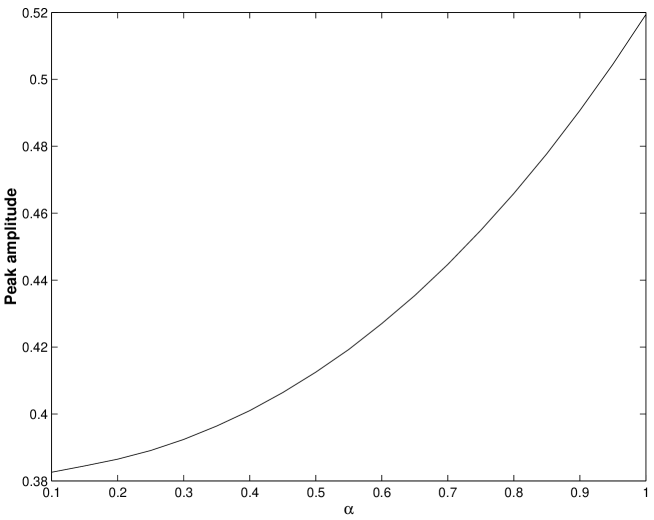
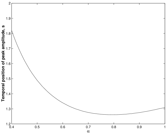
Let us choose the index $\alpha$ as a governing parameter. This means that we will change it from zero to one for establishing how it influences on the character of the system (6). The key characteristics of this system is a temporal position of the $y_{2}$’s maximum and its value. The results can be only obtained by numerical simulations. They are represented in Fig. 4 and Fig. 5. The first observation shows that the model (6) with the index $\alpha=1$ is well agreed with the models for $\alpha\neq 1$. Otherwise speaking, all they together form a smooth line in the interval $0<\alpha\leq 1$. Figure 5 has been shown for $0.4\leq\alpha\leq 1$ to be easy to recognize a minimum in this dependence on $\alpha$. Really, the minimum is the case for $\alpha\approx 0.8$. This indicates that at first the temporal position comes to the abscissa axis, when the index $\alpha$ changes from one to $\sim 0.8$. However, the next decay evolution of the index leads to the motion of the $y_{2}$’s maximum outside of the abscissa axis. The peak amplitude has a completely monotonic character depending on $\alpha$ (see Fig. 4).

Figure 5: Time position of the $y_{2}$’s maximum in the dependence of the index $\alpha$ for the nonlinear reaction with fractional dynamics .

By the concrete example we have shown that the numerical procedure of fractional integration can provide a convergent method for the solution of nonlinear systems of fractional differential equations. The approximation series solution (Adomian decomposition) is not so successful because of the too slow convergence of the corresponding series expansion for such a type of equations. Therefore, in this case the decomposition plays only a secondary role. Although the approximation series solution can be obtained to any desirable number of terms, this makes the method expensive and ineffective. Probably, it would be better to add the algorithm by an asymptotic expansion. However, it is difficult to suggest any universal method. Thus, the numerical simulations turn out to be especially useful for the analysis of nonlinear fractional differential equations.

Acknownledgement

The author expresses his sincere appreciation to Prof. K. Diethelm and Prof. N.J. Ford for their help.

References

- [1] R. L. Bagley, P. J. Torvik, J. Rheol. 27 (1983), 201-210.
- [2] R. Metzler, J. Klafter, Phys. Rep. 339 (2000), 1-77.
- [3] G. M. Zaslavsky, Phys. Rep. 371 (2002), 461-580.
- [4] K. Weron, A. Klauser, Ferroelectrics 236 (2000), 59-69.
- [5] J. T. Edwards, N. J. Ford, A. C. Simpson, J. of Comp. and Appl. Math. 148 (2002), 401-418.
- [6] K. B. Oldham, J. Spanier, The fractional calculus (Academic Press , New York, 1974).
- [7] K. S. Miller, B. Ross, An introduction to the fractional calculus and fractional differential equations (Wiley , New York, 1993).
- [8] I. Podlubny, Fractional differential equations (Academic Press , New York, 1999).
- [9] A. A. Stanislavsky, Phys.Rev. E67 (2003), 021111.
- [10] A. A. Stanislavsky, Phys.Rev. E70 (2004), 051103.
- [11] N. G. van Kampen, Stochastic Processes in Physics and Chemistry (North-Holland, Amsterdam, 1981).
- [12] A. A. Frost, R. G. Pearson, Kinetics and Mechanism (John Wiley, New York, 1961), p. 177.
- [13] M. M. Meerschaert, H.-P. Scheffler, J. Appl. Probab. 41 (2004), 623-635.
- [14] A. A. Stanislavsky, Acta Phys. Pol. 34 (2003), 3649-3660.
- [15] S. Momani, K. Al-Khaled, Appl. Math. and Comp. (2004), in print.
- [16] Yu. Rabotnov, Creep problems in structural members (North-Holland, Amsterdam, 1969), p. 129. Originally published in Russian as: Polzuchest’ Elementov Konstruktsii, Nauka, Moscow, 1966.
- [17] K. Diethelm, N. J. Ford, A. D. Freed, Yu. Luchko, Comp. Methods Appl. Mech. Eng. (2004), in print.
- [18] R. Gorenflo, I. Loutchko, Yu. Luchko, Fract. Calculus Appl. Anal. 5 (2002), 491-518. Erratum, Ibid. 6 (2003), 111-112.