Averaging the AGN X-ray spectra from deep Chandra fields

Abstract

Context. The X-ray spectra of Active Galactic Nuclei (AGN) carry the signatures of the emission from the central region, close to the Super Massive Black Hole (SMBH). For this reason, the study of deep X-ray spectra is a powerful instrument to investigate the origin of their emission.

Aims. The emission line most often observed in the X-ray spectra of AGN is Fe K_α. It is known that it can be broadened and deformed by relativistic effects if emitted close enough to the central SMBH. In recent statistical studies of the X -ray spectra of AGN samples, it is found that a narrow Fe line is ubiquitous, while whether the broad features are as common is still uncertain. We present here the results of an investigation on the characteristics of the Fe line in the average X-ray spectra of AGN in deep Chandra fields.

Methods. The average spectrum of the AGN is computed using Chandra spectra with more than 200 net counts from the AEGIS, Chandra Deep Field North (CDF-N) and Chandra Deep Field South (CDF-S) surveys. The sample spans a broader range of X-ray luminosities than other samples studied with stacking methods up to $z\sim 3.5$. We analyze the average spectra of this sample using our own averaging method, checking the results against extensive simulations. Subsamples defined in terms of column density of the local absorber, redshift and luminosity are also investigated.

Results. We found a very significant Fe line with a narrow profile in all our samples and in almost all the subsamples that we constructed. The equivalent width of the narrow line estimated in the average spectrum of the full sample is 74 eV. The broad component of the Fe line is significantly detected in the subsample of AGN with $L<1.43\times 10^{44}$ erg s^-1 and $z<0.76$, with an equivalent width 108 eV.

Conclusions. We concluded that the narrow Fe line is an ubiquitous feature of the X-ray spectra of AGN up to $\langle z\rangle\sim 3.5$. The broad component of the Fe line is significantly detected in the X-ray spectra of the AGN with low luminosity and low reshift.

1 Introduction

Table 1: Properties of the full sample and the subsamples (see text).

Sample	$N$	$N_{2-12}$	$N_{5-8}$	$\langle z\rangle$	$\langle L_{43}\rangle$	$\langle N_{h,22}\rangle$	$\Gamma$	$\chi^{2}$/dof	$\Gamma_{sim}$	$\sigma_{sim}$	EWsim
					$10^{43}$ erg s-1	$10^{22}$ cm-2				eV	eV
(1)	(2)	(3)	(4)	(5)	(6)	(7)	(8)	(9)	(10)	(11)	(12)
CDF-S	33	21561	5223	1.26	5.20	3.80	-	-	-	-	-
CDF-N	25	16134	3429	1.11	8.00	0.88	-	-	-	-	-
AEGIS	65	32971	6873	1.11	20.31	1.04	-	-	-	-	-
Total	123	70667	15526	1.15	13.82	1.75	$1.24\pm 0.05$	9.77/13	$1.897\pm 0.001$	$117\pm 1$	182
$\mathrm{log{(N_{\rm H})}}>21.5$	54	27888	7304	1.15	14.11	3.93	$0.48\pm 0.07$	8.94/13	$1.898\pm 0.001$	$129\pm 1$	190
$\mathrm{log{(N_{\rm H})}}<21.5$	69	42778	8222	1.14	13.55	0.05	$1.78\pm 0.06$	14.96/13	$1.896\pm 0.001$	$116\pm 1$	181
$\mathrm{L}_{43}<8$	74	34620	7630	0.85	2.89	1.64	$1.21\pm 0.06$	10.42/13	$1.893\pm 0.001$	$111\pm 1$	183
$\mathrm{L}_{43}>8$	49	36047	7896	1.60	30.20	1.91	$1.31\pm 0.07$	14.70/13	$1.878\pm 0.001$	$128\pm 1$	174
$\mathrm{z}<1.005$	63	34843	7507	0.70	5.43	1.28	$1.23\pm 0.06$	10.57/13	$1.896\pm 0.001$	$105\pm 1$	186
$\mathrm{z}>1.005$	60	35824	8019	1.62	22.50	2.24	$1.24\pm 0.07$	5.66/13	$1.886\pm 0.001$	$138\pm 1$	180
$\mathrm{z}<0.76$	39	23713	5285	0.57	3.23	1.17	$1.31\pm 0.07$	11.68/13	-	-	-
$\mathrm{L}_{43}<14.3$, $\mathrm{z}<0.76$	36	19007	4446	0.57	2.00	1.25	$1.29\pm 0.08$	10.99/13	-	-	-
$\mathrm{L}_{43}<14.3$, $\mathrm{z}>0.76$	49	24286	4902	1.14	5.58	1.90	$1.11\pm 0.08$	7.27/13	-	-	-
$\mathrm{L}_{43}>14.3$, $\mathrm{z}>0.76$	35	22669	5339	1.80	37.05	2.19	$1.34\pm 0.09$	11.76/13	-	-	-

The X-ray spectra of AGN are emitted from the innermost regions of the central engine, close to the central SMBH. Accordingly to the currently accepted model described in detail by Shakura et al. (1974), AGN are powered by accretion to the SMBH, with large amounts of potential energy released in the accretion disc. Assuming an optically thick, geometrically thin accretion disc, the optical-UV primary emission of the AGN is explained as the result of the thermal emission from the accretion disc.

It is well known that the emission in hard X-rays is dominated by a powerlaw with $\mathrm{\Gamma}$ $\sim 2$, and the most widely accepted interpretation for it invokes a hot plasma surrounding the accretion disc that makes inverse Compton scattering of the thermal optical-UV photons from the accretion disc (Haardt et al. (1991)).

Part of the primary emission is reflected by the accretion disc producing Compton reflection (especially significant above 10 keV) and several fluorescence lines, the most important one being the Fe $\mathrm{K}_{\alpha}$ line at 6.4 keV for neutral Fe (and 6.7-6.9 keV for Fe in the most highly ionized states), as described in Matt et al. (1991) and George & Fabian (1991). Reflection can also occur at larger scales, in the torus. The line profile gives valuable information about the emitting processes and the regions where they occur.

The study of the trend of the narrow Fe line equivalent width (EW) with continuum luminosity plays a fundamental role in the investigation of the link between the continuum emitting region and the reflecting region. A decrease of Fe line intensity with increasing continuum luminosity was found in Ginga observations of AGN ( Iwasawa et al. (1993)). The trend (the so called ”Iwasawa Taniguchi effect”, hereafter “IT effect”) was widely confirmed for both broad and narrow Fe lines by observations of ASCA, by Nandra et al. (1997), and more recently for the narrow Fe lines, for example in Bianchi et al. (2007) and Page et al. (2004), using XMM-Newton data. Although the IT effect is widely proved, the reason for the anti-correlation between the line and the continuum intensity is still under investigation: Nandra et al. (1997) attributed the IT effect to the ionization that can be important in high luminosity.

As the torus and the disc can both contribute in different measure to the observed Fe line, the resulting profile will be complex, and in particular it will depend on the inclination angle of the disc with respect to the line of sight. The estimated intrinsic column density in X-rays ($\rm N_{\rm H}$) is, in this sense, connected to the line properties: a increase of the Fe line intensity with increasing $\rm N_{\rm H}$ was found in a sample of AGN observed by Ginga and Asca (Gilli et al. (1999)). In that work, the Fe line in the spectra of the absorbed AGN (type 2 AGN) was more intense than the line found in the unabsorbed ones (type 1 AGN). This was predicted by Ghisellini et al. (1994), who performed a theoretical analysis of the Fe line in a configuration with torus and accretion disc on the same plane. In this picture, the line intensity produced by reflection and transmission in the torus increases with the $\rm N_{\rm H}$, while the continuum emission is depleted, leading to an increase of the line equivalent width for the highest $\rm N_{\rm H}$.

It should be noted that the lines produced by reflection in the torus should have a narrow and approximately Gaussian profile, while the lines produced in the accretion disc should be broadened and deformed by the effect of the newtonian movement of the gas in the accretion disc around the SMBH. It is also possible to detect in the lines the relativistic features, such as a red wing due to gravitational redshift, among other features, explained in detail in Fabian et al. (2000). These features come from the innermost regions of the accretion disc, as the relativistic effects are due to the strong gravitational field close to the central SMBH. From the study of these features it is possible to obtain the inner radius of the accretion disc, which is expected to be 6 gravitational radii ($R_{g}$) for a non-rotating BH, called a Schwarzschild BH, down to 1.23 $R_{g}$ for a maximally rotating BH, called a Kerr BH (Bardeen at al. (1972)).

Early results from ASCA showed broad and deformed lines: Nandra et al. (1997) performed a spectral analysis of a sample of local Seyferts, finding broad components in about 65% of their sample. Unambiguous broad lines were found also in more recent well exposed XMM-Newton observations of AGN (e.g. in Nandra et al. (2006), Braito et al. (2007) and Fabian et al. (2002)).

It has been proved by Guainazzi et al. (2006) that X-ray spectra with good statistical quality are necessary to detect any broad Fe line component, which would otherwise be hidden under the noise. In this context statistical methods, like summing (stacking) or averaging the spectra, have been recently introduced in X-ray astronomy to allow the study of large AGN samples including the low quality spectra that otherwise could not be well analyzed individually.

The first of such works is that of Streblyanska et al. (2005), who performed a stacking analysis on the XMM-Newton observation of the Lockmann Hole, finding a large line EW and broad line profile.

Brusa et al. (2005) stacked the spectra of CDF-N (2 Ms exposure time) and CDF-S (1 Ms exposure time) surveys by the Chandra satellite. They computed the stacked spectra in bins of redshift aiming at characterizing the Fe line emission of the sources in the X-ray background up to $z\sim 4$. They found an intense and apparently broad 6.4 keV Fe line with an EW consistent with the results of Streblyanska et al. (2005). To explain the red component, they argued that it can strongly depend on the modeling of the underlying continuum and that a spurious red wing might be produced by the contribution of absorbed spectra at different redshifts.

In recent studies of X-ray spectra using this approach, finding broad lines with relativistic profiles has been proved to be not very common, for example in Guainazzi et al. (2006) in the analysis of AGN spectra observed with XMM-Newton. They found that 25% of their sample had relativistic lines; this percentage is 50% for higher signal-to-noise ratio, selecting only spectra with large numbers of counts. Moreover, they found the strongest relativistic profiles in low luminosity objects.

Corral et al. (2008) averaged the XMM-Newton spectra of type 1 AGN, using the AXIS (Mateos et al. (2005)) and XWAS (Mateos et al. (2010)) samples, up to redshift $\sim$ 3.5. They found a narrow Fe line, while no clear evidence of a broad line was found. The reason for the discrepancies between this work and that of Streblyanska et al. (2005) can be explained considering the differences of the samples, as the Corral et al. (2008) sample has higher luminosities (and therefore lower predicted EWs, following the IT effect) and less spectral counts, including more noisy sources. Another reason for the discrepancy can be found in the method, since Corral et al. (2008) estimate the continuum shape using simulations, while in Streblyanska et al. (2005) it was not constructed and subtracted in the same way and this could introduce some uncertainties. Moreover, Streblyanska et al. (2005) binned the spectra before stacking them, and Yaqoob (2006) showed that this procedure can introduce features like a broad red tail in an emission line.

A stacking analysis of a deep and complete sample of 507 AGN with $z<4.5$ defined from the 2XMM catalogue was performed by Chaudhary et al. (2010). They were able to characterize the properties of the stacked spectrum of the AGN, such as the Fe line shape and the dependence of its intensity with X-ray continuum luminosity and the redshift. They found a clear evidence of a narrow neutral Fe line, and they confirmed the IT effect in AGN over a broad range of redshift.

Recently, a stacking analysis on XMM-Newton X-ray spectra of the COSMOS sample was performed (Iwasawa et al. (2011)): they found an excess on the high-energy side of the Fe line, interpreted as the convolution of narrow lines from ionized Fe.

In summary, according to recent results, while the narrow Fe lines are commonly detected in the spectra, clear evidence for relativistic lines is rare. The paucity of relativistic lines is a problem, as they are expected in the accretion disc scenario. There are a number of possible solutions for this problem. The first one invokes the presence of ionized discs (Iwasawa et al. (2011), Matt et al. (1996)); the second solution explains it with the presence of fastly spinning BH (Iwasawa et al. (1996) and Fabian et al. (2002)): in this case the lines would be very broad and sometimes difficult to separate from the continuum. The last explanation for the lack of broad lines postulates truncated discs, as found by Matt et al. (2005).

We present in this paper a stacking analysis of a comprehensive sample of absorbed and unabsorbed AGN in the deepest Chandra surveys: AEGIS and Chandra Deep Fields. We followed the method presented by Corral et al. (2008), and we accurately tested and adapted it for Chandra spectra, in order to carefully check our results. The Chandra sample in this work allows us to explore the properties of AGN with the best statistics ever reached at high redshift, as it is deeper than the XMM-Newton samples that have previously been analyzed with stacking techniques, such as Corral et al. (2008) and Chaudhary et al. (2010) (see Sect. 2.2). In comparison with the previous stacking analysis of the Chandra samples in Brusa et al. (2005), we include the sources from the AEGIS-X survey, improving the statistics of high luminosity AGN, and we use the more recent (2 Ms) observation of the CDFS (Sect. 2.1).

The paper is organized as follows: the properties of the sample are described in Sect. 2; the method in Sect. 3; discussion of the results is in Sect. 4; we summarize the conclusions in Sect. 5.

Across this paper, we adopt the cosmological parameters: $H_{\ 0}$=70 km s^-1 Mpc^-1; $\Omega_{\lambda}$=0.7 (Komatsu et al. (2011)).

In this paper, all the counts refer to the net number of counts between 2 and 12 keV rest-frame; all the luminosities are calculated between 2 and 10 keV rest-frame and are corrected for Galactic and intrinsic absorption using the fits to the individual spectra (see below). We have used XSPEC v. 12.5 (Arnaud, (1996)) for spectral analysis.

2 X-ray samples

The X-ray results presented in this paper are obtained from the Chandra observations of the AEGIS, CDF-N and CDF-S surveys.

2.1 Parent Chandra surveys

The AEGIS-X survey is a Chandra survey of the Extended Groth Strip (EGS) region, designed primarily for studying the co-evolution of black holes and their host galaxies. The data we used are the result of 8 contiguous Advanced CCD Imaging Spectrometer (ACIS-I) pointings, each with exposure 200 ks, totalling 1.6 Ms. The survey covers a total area of approximately 2302 arcmin² a in a strip of length 2 degrees. The total number of identified sources with spectroscopic redshifts is 409. The data reduction and point source detection algorithms used to analyze these data are described in Laird et al. (2009).

The Chandra Deep Field-North (CDF-N) survey is one of the deepest (2Ms with ACIS-I) 0.5-8.0 keV surveys ever made: nearly 600 X-ray sources are detected over 448 arcmin². The total number of sources identified with spectroscopic redshifts is 307. Details of data reduction and the point source catalog are described in the paper by Alexander et al. (2003).

The Chandra Deep Field South (CDF-S) is the deepest and most sensitive observation obtained with Chandra. We used the 2 Ms survey, covering an area of 436 arcmin². Several hundred X-ray point sources were detected. The number of sources identified with spectroscopic redshifts is 152. A detailed description of the survey can be found in the paper Luo et al. (2008). It has been recently extended to 4 Ms, as described in Alexander et al. (2011), and Xue et al. (2011).

2.2 Sample definition and properties

Our main purpose is to study the average spectrum of AGN in the 2-12 keV energy band (rest-frame), and to determine the shape of the Fe line at $\sim$6.4 keV. The X-ray spectra of our sample have few counts and do not allow a detailed analysis of the individual spectra, except for a handful of sources. For the detection of any relativistically broadened component, as underlined by Guainazzi et al. (2006), it is necessary to have good quality spectra, hence we need to improve the signal-to-noise ratio.

To increase the probability of detecting any broad component that otherwise would be hidden by the noise, we included in our analysis only those sources with more than 200 counts. We discuss in Appendix A the results corresponding to lower thresholds (50 and 100 counts). We further selected only sources with spectroscopic redshifts. Finally, we excluded from our analysis also two sources with more than 10000 counts individually: CDFS_-056 (RA: 53.112, DEC: -27.685), CDFN_-141 (RA: 189.1, DEC: 62.383). These sources have such a strong signal in their spectra that they would largely dominate the average stracked spectrum.

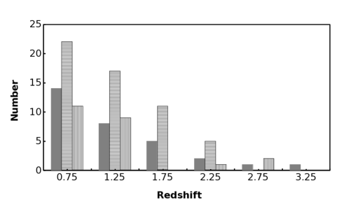
Our full sample contains 123 sources with spectroscopic redshifts and more than 200 counts each (but less than 10000 cts), with 70667 counts in total (see Table 1). The distribution of the net counts per source for this full sample is shown in Fig.1. The redshift distribution of the sources is shown in Fig. 2, where we can see that our sample spans a broad range of redshifts from $z=0$ up to $z=3.5$.

Figure 1: Distribution of the net counts between 2 and 12 keV rest-frame. Filled histogram: CDF-S; histogram with horizontal stripes: AEGIS, histogram with vertical stripes: CDF-N.

Figure 2: Redshift distribution. Filled histogram: CDF-S; histogram with horizontal stripes: AEGIS, histogram with vertical stripes: CDF-N.

Source and background spectra, and their ancillary and response matrices were extracted for each source (Digby-North, (2011)), using the tool ACIS-EXTRACT, version 2008-03-04, Broos et al. (2010). Before spectral fitting, all the spectra were grouped with a minimum of 5 counts per bin, and we applied the modified Cash statistics discussed in the XSPEC pages . This grouping was adopted because we used the same method for all the sources with more than 50 counts (see Appendix A), for which the more common $\chi^{2}$ statistics would not be adequate.

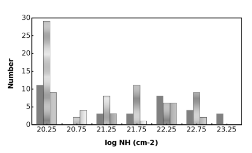
It should be noted that in this step we did not aim at making a detailed analysis of the individual spectra but rather only at obtaining a set of parameters that we use to unfold the spectra for all the instrumental effects (see Sect. 3). The model is a single power law modified by Galactic absorption (with fixed values at 1.4 $\times\rm 10^{20}\rm cm^{-2}$ for AEGIS, 0.772 $\times\rm 10^{20}cm^{-2}$ for CDF-S, 0.993 $\times\rm 10^{20}\rm cm^{-2}$ for CDF-N) plus intrinsic absorption at the redshift of each source. We left the slope of the power law, its normalization and the intrinsic column density as free parameters. The fit was performed in the rest-frame energy range between 1 and 12 keV, minimizing the contribution from any putative soft excess present in the sources. The resulting distribution of intrinsic column densities is shown in Fig.3. Most of the highly absorbed sources belong to CDF-S, as indicated by the higher average column density for that sample in Table 1.

2.3 Subsample definition

Figure 3: Distribution of intrinsic column density in units of $10^{22}$ cm^-2 . Filled histogram: CDF-S; histogram with horizontal stripes: AEGIS, histogram with vertical stripes: CDF-N. We grouped the spectra with $\rm log(N_{\rm H})<10^{20}$ with the spectra having $\rm log(N_{\rm H})=10^{20}$.

Figure 4: Distribution of rest-frame 2-10 keV luminosities in units of erg s^-1. Filled histogram: CDF-S; histogram with horizontal stripes: AEGIS, histogram with vertical stripes: CDF-N.

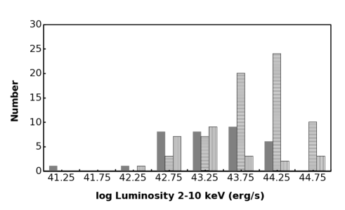
We show in Fig. 4 the distribution of the X-ray luminosities of the sources corrected for Galactic and intrinsic absorption, calculated from the fit to the indvidual spectra. The average luminosity of the AEGIS sources is one order of magnitude higher than the average luminosity of CDF-N and CDF-S sources (Table 1).

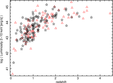
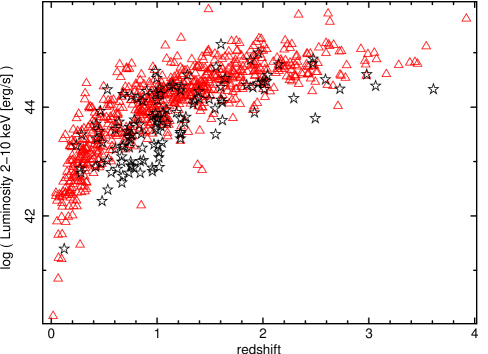
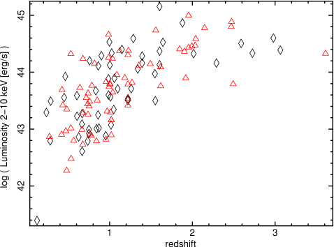
We compared the distribution of our ful sample in the luminosity-redshift plane with that of Streblyanska et al. (2005) in the Lockmann Hole (Fig. 5): we sample better that plane at $z<3$ for all luminosities. Compared to the Corral et al. (2008) sample (XMS-XWAS) (Fig. 6) we cover about one order of magnitude lower luminosities for $0.5<z<3$. Finally, with respect to Brusa et al. (2005), the addition of the AEGIS sample and the restriction to sources with high numbers of counts, allows us to span a broader range of luminosities at similar $z$. In summary, our sample combines a unique combination of deep coverage with high z sources, a broad span of luminosities and good statistics.

Figure 5: Comparison of our full sample (black stars) with the deep XMM-Newton sample of Streblyanska et al. (2005) (LH, red triangles), in the luminosity-redshift plane.

Figure 6: Comparison of our full sample (black stars) with the medium XMM-Newton sample of Corral et al. (2008) (XMS+XWAS, red triangles), in the luminosity-redfhit plane. For clarity, we omitted one XMS+XWAS source of XMS+XWAS at $z=2.34$, $L=1.28\times 10^{47}$ erg s^-1.

Figure 7: Distribution of the unabsorbed (red triangles) and absorbed (black diamonds) subsamples (see Sect. 2.3) in the luminosity-redshift plane.

Figure 8: Distribution of the $L-z$ subsamples (see text) in the luminosity-redshift plane. The dividing point is $z=0.76$, $L=1.435\times 10^{44}$ erg s^-1 (marked by the horizontal and vertical solid lines). The three blue stars mark the sources that allow defining distinct $L-z$ subsamples (see text).

One of the main aims of our work is to understand the dependence of the spectral properties of the AGN on luminosity, redshift, and intrinsic absorption. For this reason, we performed the analysis of the stacked spectra not only for the full sample, but also for subsamples defined in terms of column density, luminosity, and redshift. Except for $N_{\rm H}$ (see below) the bins have been designed to have a similar numbers of total counts each. The characteristics of each subsample can be seen in Table 1.

• Intrinsic $N_{\rm H}$: The threshold column density was set at $\log(N_{\rm H}/{\rm cm}^{-2})=21.5$ as the absorption features of the X-ray spectra are detected in the AGN with $\log(N_{\rm H}/{\rm cm}^{-2})>21.5$. Local absorbers with $\log(N_{\rm H}/{\rm cm}^{-2})=21.5$ are opaque for $E<1$ keV and transparent for $E>1$ keV. The transition energy between the transparent and opaque regime linearly grows with $N_{\rm H}$, until $N_{\rm H}\sim 10^{24}\rm cm^{-2}$, where the Compton Thick regime dominates. We show in Fig. 7 the distribution of the absorbed and unabsorbed subsamples just defined: the two subsamples have a similar distribution in the luminosity-redshift plane, so they are fair representations of the AGN with and without absorption, with no other parameters playing an important role (see also Table 1).

• Luminosity: We separated high and low luminosity sources using a threshold $L=8\times 10^{43}$ erg s^-1

• $z$: We built a low-$z$ and a high-$z$ subsample with a threshold $z=1.005$

• $L-z$: Initially we divided the full sample in three subsamples: (i) $z<0.76$ (hereafter low $z$-low $L$) (ii) $z>0.76$ and $L<14.35\times 10^{43}$ erg/s (hereafter high $z$-low $L$) (iii) $z>0.76$ and $L>14.35\times 10^{43}$ erg/s (hereafter high $z$-high $L$). In the low $z$-low $L$ subsample there are only 3 sources above $L<14.35\times 10^{43}$ erg/s (with $\sim$4000 total counts), so we have also used a second version of this subsample using only sources with $z<0.76$, $L<14.35\times 10^{43}$ erg/s so that this subsample and the two high $z$ subsamples cover distinct $z$ and $L$ intervals. All results are very similar and we have used the latter definition of distinct areas as our default.

3 Analysis method

3.1 Averaging method

Our averaging method was presented for the first time in Corral et al. (2008) for the XMM-Newton spectra of XMS-XWAS surveys; it was then also used for the study of the XBS sample by Corral et al. (2011). We adapted and tested it for the Chandra spectra.

After fitting the spectra as described in Sect.2.2, we read into XSPEC again each un-binned, background-subtracted spectrum, we applied the corresponding best fit model and we extracted the unfolded spectra taking into account the detector response (eufspec command in XSPEC). In this step it is possible that some distortions to narrow spectral features were introduced, such as to the Fe emission line. In order to quantify this effect, we performed extensive simulations of the continuum and of the Fe Line as described in Sect.3.2 and 3.3. Once we obtained all the unfolded spectra, the following step was to apply the corrections described in Corral et al. (2008) that we can summarize as follows:

1. Correction for Galactic absorption

2. Shift the spectra to a common redshift frame

3. Re-normalize the spectra with respect to the integrated flux between 2 and 5 keV restframe

Once we obtained the de-absorbed and re-normalized spectra at rest-frame, we re-binned each spectrum. For simplicity, we used the same binning for all the average spectra, applying the bin definitions of the absorbed sample: this binning was constructed in order to have at least 1000 net counts in each bin of the co-added spectrum. In order to maximize our ability to detect a narrow Fe line, we always centered one bin at 6.4 keV. We finally averaged the spectra using the unweighted arithmetic average.

Figure 9: Average observed spectrum of the full sample fitted with a powerlaw between 2 and 5 keV.

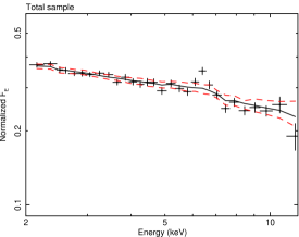
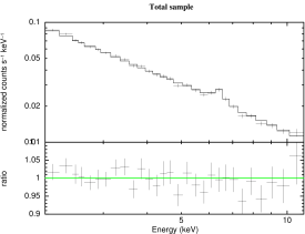
We show in Fig. 9 the average spectrum of the total sample. If we fit the 2-5 keV range with a powerlaw and extrapolate it to the full range, an excess can be clearly seen around the expected position of the Fe emission line. However, any features found in the average spectra must be carefully evaluated, as the averaging procedure itself may introduce some distortions. For this reason, we computed the continuum using simulations, as described below.

3.2 Simulations of the continuum

Previous works, as for example Yaqoob (2007) and Corral et al. (2008), have shown that the unfolding and the averaging process can distort the shape of the spectrum. Therefore, it is important to take this into account before deriving conclusions from the spectral analysis of the average spectrum.

In order to characterize the underlying continuum of our sample, we made 100 simulations of each source using the best fit parameters of the continuum model (see Sect. 2.2). To each of these 100 simulated samples we applied the same method as the one used for the observed sample (spectral fitting, correcting for response, correcting for Galactic absorption and z, rescaling and averaging). After this, we represented our continuum with the median of the 100 averaged simulated continua. We decided to use the median and not the arithmetic average as it is a more robust estimate of a central value and in particular it is less sensitive to extreme values. Hereafter we will call this the simulated continuum.

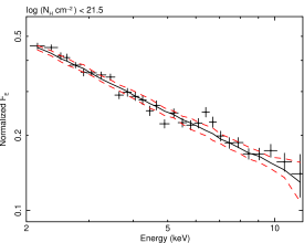
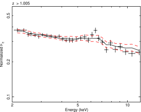
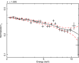
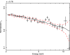
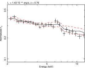
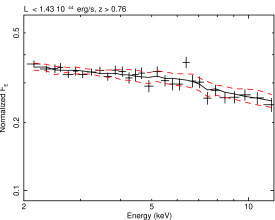
We represent in Figs. 10, 11, 12, 13, and 14 the average observed spectra (dots with error bars), along with the simulated continua (solid lines), and the 1 sigma confidence limits (dashed lines). The latter correspond to the 16th and 84th element of the sorted fluxes of the simulated spectra at each bin. Features around the expected location of the Fe K line are conspicuous in all the subsamples.

Before attempting to draw any conclusions from those features, we have characterized the effect of our averaging method on narrow lines using simulations, as described in the next section.

Figure 10: Average observed spectrum of the full sample (data points) with the average simulated continuum (continuous line) and the one sigma confidence limits (dashed lines).

Figure 11: Average observed spectra (data points) of the absorbed (left) and unabsorbed (right) subsample with their average simulated continua (continuous line) and the one sigma confidence limits (dashed lines).

Figure 12: Average observed spectra (data points) of the high-$z$ (left) and low-$z$ (right) subsamples with their average simulated continua (continuous line) and the one sigma confidence limits (dashed lines).

Figure 13: Average observed spectra (data points) of the high-$L$ (right) and low-$L$ (left) subsamples with their average simulated continua (continuous line) and the one sigma confidence limits (dashed lines).

Figure 14: Average observed spectra (data points) of the $L-z$ subsamples with their average simulated continua (continuous line) and the one sigma confidence limits (dashed lines). For comparison, in the bottom-left panel we represent with a dotted line the result of adding to the simulated continuum a Gaussian centered at 6.4 keV, with $\sigma$=120 eV, as obtained from the simulations of the Fe line (Sect. 3.3).

3.3 Simulations of the Fe Line

We performed simulations of unresolved Fe lines in order to study how the spectral resolution of ACIS-I and the averaging process widen the narrow spectral features in X-ray spectra.

We simulated high signal to noise spectra (one simulation for each spectrum, without Poissonian noise) using a powerlaw with $\Gamma$ fixed at 1.9, with unit normalization, and a zero sigma Gaussian. The input EW was 200 eV and energy fixed at 6.4 keV, at the $z$ of each source. We made the correction for the response (using a power law with Gamma fixed at 1.9) and we finally computed the average spectrum with the same treatment applied to the real spectra.

We show in columns $\Gamma_{\mathrm{s}imline}$, $\sigma_{\mathrm{s}imline}$ and EW of Table 1 the results of fitting a powerlaw plus a Gaussian to these simulations for some of the samples. The EW and powerlaw slope are recovered very well. The width of the line has become $\sigma\sim 120$ eV. Therefore, our resulting “instrumental resolution” is around 120 eV, i.e., any real detected feature around rest-frame 6.4 keV should be wider than this value and its actual width will be the convolution of its intrinsic width with this value, roughly added in quadrature (see Eq. 1 below).

We show in the bottom-left corner of Fig. 14 the expected profile of an unresolved 6.4 keV line added to the simulated continuum for the corresponding subsample. In general, the features we observe around that energy appear to be compatible with such an unresolved line, except perhaps for the low $z$-low $L$, high $z$-high $L$ and high $L$ subsamples. We will quantify these qualitative impressions in Section 4.2.

4 Results

In this section we study the statistical significance of the Fe line and its properties in several steps. We first developed a model-independent way to calculate the significance of the line detection (Sect. 4.1), then we studied again its significance and characteristics fitting the average spectra using a single Gaussian to fit the Fe line (Sect. 4.2). In Sect. 4.3 we study the dependence of the line on $z$ and X-ray luminosity. Finally, in Sect. 4.4 we try complex line models with those subsamples that show significant broad line profiles.

4.1 Significance from the simulations

In order to estimate the significance of the excess observed in the Fe K line region, we calculated the percentage of average simulated spectra (from the simulations of the continuum described in Sect. 3.2) having a flux in the Fe K region which is lower than the flux of the observed spectrum. We should note that this method does not depend on a modeling of the continuum (as in the calculation of the equivalent width, in the next Section). The Fe line flux was calculated in three regions centered at 6.4 keV, with half-widths of 0.1 keV, 0.2 keV, and 0.4 keV respectively. The significances of the Fe line estimated in this way for the full sample and all subsamples are in Table 2.

The narrowest interval was chosen at the limit of the instrumental broadening, a significant excess found just in this range and not in the other two would in principle correspond to a detection of a narrow line. On the other hand, increasing the width includes more flux from a putative broad line, but it also increases the noise, hence a broad component would be more difficult to detect. We use the $\pm 0.2$ keV wide option (column $S_{2}$ in Table 2) as our fiducial value, since it maximizes the signal-to-noise ratio for unresolved and moderately broad lines. We can see that the line is strongly significant ($>98$ %) in the full sample and in almost all the subsamples, with the exception of the high $z$-high $L$ one. In general, the significance is higher for low $z$ and low $L$.

In all cases, the significance stays about the same or decreases when $\Delta E$ increases. This is either an effect of the expected lower signal-to-noise ratio for wider intervals, or might indicate the presence of a wider profile in the cases where the significance does not decrease noticeably.

Table 2: Significance of the Fe line estimated from the simulations for the full sample and the subsamples.

Sample	$S_{1}$	$S_{2}$	$S_{3}$
	(1)	(2)	(3)
Total	100	100	99
$\mathrm{log{(N_{\rm H})}}>21.5$	99	99	98
$\mathrm{log{(N_{\rm H})}}<21.5$	100	100	100
$\mathrm{L}_{43}<8$	100	100	100
$\mathrm{L}_{43}>8$	97	98	96
$\mathrm{z}<1.005$	100	100	100
$\mathrm{z}>1.005$	98	98	98
$\mathrm{L}_{43}<14.3$, $\mathrm{z}<0.76$	100	100	100
$\mathrm{z}<0.76$	100	100	100
$\mathrm{L}_{43}<14.3$, $\mathrm{z}>0.76$	99	98	91
$\mathrm{L}_{43}>14.3$, $\mathrm{z}>0.76$	88	88	86

4.2 Spectral fits on the full sample and subsamples

After having made the above mentioned calculation of the significance of the Fe line, we performed the spectral analysis. To do this, we represented the continuum using the simulated continuum as a table model in XSPEC. During the fits described below, we have aways left its normalization free to vary, and its value returned in XSPEC is always around one. We added to the table model the required components when we found residuals. We used the goodness of fit criterion and the confidence interval for a given parameter corresponding to a $\mathrm{\Delta}\chi^{2}=2.71$ (90 % probability). The fit results are shown in Table 3.

The $\sigma$ we mention in the remainder of this work (including Table 3), refers to the intrinsic width of the line, taking into account the broadening introduced by our method

$$\sigma^{2}=\sigma^{2}_{obs}-\sigma^{2}_{sim}$$ (1)

where $\sigma_{obs}$ is the total width returned by XSPEC and $\sigma_{sim}$ is the instrumental width obtained from the simulations of an unresolved Fe K line (120 eV, see Sect. 3.3.). During the fits, we forced the width of the Gaussian line to satisfy the condition: $\sigma_{obs}\geq\sigma_{sim}$ (where we used the average value of $\sigma_{sim}$ reported in Table 1, that is approximately 120 eV).

We made the fits in several steps:

• Fixed $\sigma$=0 and fixed centroid energy at 6.4 keV: this allows us to estimate the significance of the narrow component of a neutral Fe K line (first line for each sample in Table 3)

• Fixed centroid energy at 6.4 keV and free $\sigma$: studies the significance of a possible broad component and constrains its width (second line for each sample)

• Free centroid energy and fixed $\sigma$=0: considers the presence of an ionized narrow Fe component and estimates its centroid energy (third line for each sample)

• Free centroid energy and free $\sigma$: leaves all options open (fourth line for each sample)

We calculated the significance of the Gaussian with the $\Delta\chi^{2}$ corresponding to the fits with and without the line component, and we checked the corresponding probability using the incomplete $\beta$ function (according to Press et al. (2007)). The result is in Col. 4 in Table 3. In the same way, we estimated the significance of allowing the width and/or the centroid energy to vary with respect to the baseline narrow and neutral line.

We summarize here the results for our (sub)samples (see Table 3 and Figs. 15, 16, 17, 18, and 19) :

• Full sample:
  The spectrum of the full sample fitted with the table model and the Gaussian with free energy and free $\sigma$ are shown in Fig.15. We can see that the model fits the spectrum well in the Fe line region. The detected line is narrow. We do not observe any ionized Fe line component.

• Absorbed and unabsorbed subsamples:
  The spectra and fitted models are shown in Fig.16. The continuum of the unabsorbed sample shows $\Gamma\sim 1.8$, a common value for the AGN (see Table 1), and is flatter in the absorbed sample, as expected. The line is characterized by having a narrow profile for both subsamples. Only in the unabsorbed sample the centroid energy of the line might suggest a contribution from mildly ionized Fe. However, the centroid energy is consistent with 6.4 keV within the 90 % confidence level, and the significance of $\sigma>$0 from the $\Delta\chi^{2}$ is $<$ 90 %.

• High and low luminosity subsamples:
  The spectra and fitted models are shown in Fig. 17. The results of the fits suggest a more intense Fe line in the low-$L$ subsample. We discuss the dependence of the EW on redshift and luminosity more in detail in the next Section. The detected line is narrow, and there is no significant ionized Fe contribution.

• High and low redshift subsamples:
  The spectra and fitted models are shown in Fig. 18. The Fe line is more significant at low redshift than at high redshift and this can reflect the same trend just found with the luminosity, since sources with higher $L$ are preferentially found at higher $z$. The line profile is narrow in both cases. The fits with the centroid energy free shows the presence of a mildly ionized Fe contribution in the low redshift sample, but 6.4 keV is within the 90 % confidence interval.

• $L$-$z$ subsamples:
  The strongest line significance is found at low $z$ and low $L$, then decreasing with both redshift and luminosity. The line profile is broad only in one case, in the low redshift- low luminosity sample ($>$95.4 % probability). The line profile looks symmetric (see Figs. 14 and 19, two left panels). This suggests reflection from regions in newtonian movement in the accretion disc, although we can not exclude the relativistic profile. Moreover, in the top-left panel there seems to be an excess in the narrow bin around 6.4 keV, which might come from an additional narrow component. We discuss in more detail the shape of this feature in Section 4.4. In the other two subsamples, the detected profile of the Fe line is narrow. We did not find any ionized Fe component.

At high energies ($\sim$ 10 keV), we observed in some spectra an excess that can be interpreted as part of the Compton reflection. The paucity of counts at these energies does not allow us to make a more accurate assessment of this continuum component. An absorption feature was also detected, to some extent, in some of our average spectra around 7-8 keV: this can be explained as the Fe edge commonly found along the Compton reflection component.

Figure 15: Fit of the average spectrum of the full sample using the simulated continuum model + Gaussian (with free $\sigma$ and free centroid energy)

Figure 16: Fit of the average spectrum of the absorbed (left) and unabsorbed (right) subsamples using the simulated continuum model + Gaussian (with free $\sigma$ and free centroid energy)

Figure 17: Fit of the average spectrum of the low luminosity (left) and high luminosity (right) subsamples using the simulated continuum model + Gaussian (with free $\sigma$ and free centroid energy)

Figure 18: Fit of the average spectrum of the low redshift (left) and high redshift (right) subsamples using the simulated continuum model + Gaussian (with free $\sigma$ and free centroid energy)

Figure 19: Fit of the average spectrum of the $L-z$ subsamples (low $L$-low $z$ subsamples in the left panels, low $L$- high $z$ subsamples in the right bottom panel, high $L$-high $z$ subsample in the right top panel) using the simulated continuum model + Gaussian (with free $\sigma$ and free centroid energy)

4.3 Dependence on redshift and luminosity

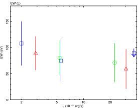
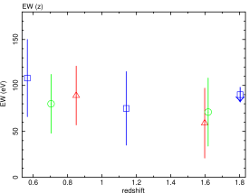
As our results seem to suggest a dependence of the Fe line EW on redshift and on luminosity, for low $z$ and low luminosity AGN, we checked this result in more detail to understand it better. The distribution of the line EW with the average $z$ and the average luminosity of the subsamples are shown in Fig. 20. In those figures, the same symbols refer to statistically independent subsamples. On the contrary, subsamples with different symbols are not statistically independent and there will be significant overlapping among the sources included in each subsample. We have used the fits corresponding to an unresolved line fixed at 6.4 keV (first line for each subsample in Table 3).

At first view the EW seems to decrease both with increasing $z$ and X-ray luminosity. However, looking for example at the blue squares (corresponding to independent $L-z$ subsamples), it is clear that a constant EW is consistent with the data points the upper limits and, hence, the trend, albeit suggestive, is not statistically significant.

Figure 20: Dependence of unresolved 6.4 keV Fe line equivalent width with the average luminosity (left) and the average redshift (right) of the subsamples (first row of Table 3). Squares: $L-z$ subsamples; circles: redshift subsamples; triangles: luminosity subsamples. We represent upper limits with a down-pointing arrow. Each set of points with the same symbol are statistically independent, but not so across symbols.

4.4 Analysis of broad lines

We detected with strong significance narrow Fe K lines in all samples. Additionally, in the low $L$-low $z$ subsample, the Fe line appears significanlty broadened with a significance above two sigma). We investigate here whether relativistic profiles are better fits than a simplistic broad Gaussian.

We added to the simulated continuum the diskline model in XSPEC which describes a relativistically broadened emission line for an accretion disc around a Shwartzschild Black Hole. We fixed $R_{out}$, the external radius of the accretion disc, to $1000\,R_{g}$. We left $R_{in}$, the inner radius, free to vary, obtaining an upper limit for it: $<142\,R_{g}$. As mentioned in Sect. 1, the inner radius of the accretion disc is expected to be lower ($6\,R_{g}$ for a non-rotating black hole and $1.23\,R_{g}$ for a maximally-rotating one). The EW is consistent with the one obtained in the fit with the Gaussian (see Table 3): EW=$152^{+70}_{-70}$ eV. The significance of adding an Fe line with diskline to the continuum is $>99.99$%, again consistent with the case of the Gaussian (Table 3). The fit gives $\chi^{2}/$dof=20.53/29, to be compared with $\chi^{2}$/dof=19.07/25 for the Gaussian: the fit is not better with more free parameters. Summarizing, the diskline fits the Fe K line as well as the Gaussian: we do not significantly detect a definite relativistic profile in the line, although it cannot be excluded.

Alternatively, the profile of the line could be characterized as the sum of both a broad and a narrow components since, in principle, we would expect a contribution from both a torus (narrow component) and disk (broad component) reflections.

We have assessed the significance of this possibility by making a final test in the low $L$- low $z$ sample: we added a broad Gaussian to the narrow Gaussian (i.e. combining models in the first and second line of Table 3). We fixed the centroid energies of the two Gaussians at 6.4 keV and we fixed the $\sigma$ to zero in the narrow Gaussian and to 240 eV (the value in the second line in Table 3) in the second broad Gaussian.

We calculated the EW of the narrow and broad components, obtaining $<84$ eV and $158^{+78}_{-78}$ eV, respectively. This fit gives $\chi^{2}$/dof=19.15/26, to be compared with $\chi^{2}$/dof=23.70/27 of the fit with only narrow Gaussian (in Table 3). Hence, the significance of adding the broad component ($\Delta\chi^{2}$=4.55 and $\Delta\nu$=1) is $>95.4$% but $<99$%, calculated as mentioned in Sect. 4.2. We conclude that a double Gaussian is a better fit, but only at the $2\sigma$ level.

5 Conclusions

We have studied the average spectrum of a sample of 123 AGN with more than 200 net counts selected from the Chandra AEGIS, CDF-N and CDF-S surveys, covering $\mathrm{0}<z<3.5$ and totalling $>$70000 cts. Compared to similar XMM-Newton and Chandra studies of deep fields, we sample better the luminosity-redshift plane at $z\leq 3$ (including higher luminosities) and use deeper CDF-S data. With respect to shallower wider surveys using XMM-Newton, we reach about an order of magnitude lower luminosities over the same redshift range.

To improve the signal-to-noise ratio and to study the average properties of the sample, we computed its average spectrum, adapting the method developed by Corral et al. (2008). We constructed the continuum model with simulations, in order to accurately analyze our resulting spectra. We also assessed the effect of our averaging method on unresolved features around 6.4 keV, to obtain the intrinsic widths of any putative lines.

We repeated the averaging procedure for the subsamples defined in two intervals of column density, 2-10 keV X-ray luminosity, redshift, and in three 2D intervals in the luminosity-redshift ($L-z$) plane (see Table 1).

We have estimated the significance of the presence of narrow and broad features around 6.4 keV in a model-independent way (Table 2), finding that narrow features are significant at $\geq$98%, except for the high-$L$, high-$z$ subsamples, where it is lower. Broad features would be harder to detect and are most significant at low $L$ and low $z$.

Analyzing the spectra with XSPEC using the simulated continuum and modelling the Fe line as a Gaussian, we have found strong evidence of a narrow Fe line at high significance in our full sample and in most of our subsamples, in particular (Table 3):

• We detected a strong (at $>99.73$ %) narrow Fe line with EW$=85\pm 35$ eV and $73\pm 32$ eV in the absorbed and unabsorbed subsamples, respectively (defined as having intrinsic column density above and below $10^{21.5}$ cm^-2, respectively), with a hint of higher central energy $\sim$6.5 keV in the unabsorbed case, but still compatible with 6.4 keV at 90%.

• Segregating the sources purely on luminosity, we found that the average spectrum in the low-$L$ ($L<8\times 10^{43}$ erg s^-1) subsample shows a significant and strong narrow Fe line (EW$=89\pm 32$ eV at $>$99.99%). The significance and strength of the high-$L$ are clearly smaller: EW$=59\pm 38$ eV at 95.4%.

• Separating instead at $z=1.005$, the narrow Fe line is again stronger in the low-$z$ subsample (EW$=80\pm 32$ eV at $>$99.99%) than in the high-$z$ subsample (EW$=71\pm 37$ eV at $>$99.73%) but the difference is not significant

• Defining distinct areas in the $L-z$ plane (the division point was $L=14.3\times 10^{43}$ erg s^-1,$z=0.76$), the most significant line is found in the low $L$-low $z$ subsample (EW$=108\pm 42$ eV at $>99.99$%), with a hint of a broad component ($\sigma=240\pm 90$ eV at $>2\sigma$ significance). The low $L$-high $z$ subsample also shows a somewhat weaker narrow line (EW$=75\pm 40$ eV at $\sim 99.7$%). The Fe line detection is at $<90$% significance in the high $L$-high $z$ subsample (EW$<90$ eV)

We studied the trend of the EW for the narrow Fe line with redshift and luminosity of our subsamples. We did not find a significant dependence: in Fig. 20 that trend is not statistically more significant than a constant. In order to disentangle the effects of the two parameters on the line detection, surveys of AGN covering a wider area in the $L-z$ plane are needed. Since the Fe line is detected more significantly at low-$L$ and low-$z$, samples of the local Universe are particularly suited to this end.

We have also investigated whether more sophisticated models for the line profile would provide a better fit, concentrating on the low $L$-low $z$ subsample, since it is the only one where a broad line may have been detected. A diskline relativistic profile provides a worse fit than a broad Gaussian, with more parameters. Additionally, the inner radius of the disk would be too large to produce significant relativistic effects. Therefore, we do not find evidence for a relativistic profile in any of our average spectra.

However, as has been pointed out in Guainazzi et al. (2006), in the average spectra the broad component of the observed line comes from a maximum $\sim 50$% of the sample: the line in an average spectrum cannot have a relativistic profile as definite as the one that can be in principle observed in a single, good quality spectrum. In particular, there can be a contribution from partially ionized Fe that produces narrow lines at energies $>$ 6.4 keV, up to $\sim$7 keV if the Fe is completely ionized. Our observed $\sim$symmetric Gaussian profile may hence be a combination of many mildly ionized Fe lines with a red wing, perhaps from relativistic effects. As mentioned in Sect. 1, a similar result has been recently found in the stacking of the X-ray spectra of the COSMOS sample (Iwasawa et al. (2011)).

Allowing for both a narrow (from neutral material far away from the central source, e.g. the putative torus) and a broad Gaussian (as just discussed) components provides a better fit than a single narrow or broad Gaussian, but with a modest significance $<99$%.

Further spectral averaging studies with higher statistics covering a wider range of source properties would allow a more detailed characterization of the Fe feature in the X-ray spectra of AGN, and whether it depends on cosmic time, intrinsic brightness, amount of surrounding material, black hole mass, accretion rate, and other physical parameters, helping to constrain the physical properties of AGN throughout the history of the Universe.

Table 3: Results of fits of the average spectrum of the full sample and its subsamples.

Sample	$\chi^{2}$/dof(s)	$\chi^{2}$/dof(g)	$P_{1}$	$P_{2}$	E	$\sigma$	EW	$\langle z\rangle$	$\langle L_{43}\rangle$	$N_{h,22}$
			%	%	keV	eV	eV		$10^{43}$erg s-1	$10^{22}cm^{-2}$
(1)	(2)	(3)	(4)	(5)	(6)	(7)	(8)	(9)	(10)	(11)
Total	47.50/28	23.74/27	$>99.99$		6.4	0	$74\pm 24$	1.15	13.80	1.75
		21.98/26	$>99.99$	$<90$	6.4	$<138$	$94\pm 30$
		23.74/26	$>99.99$	$<90$	$6.40\pm 0.10$	0	$73\pm 25$
		21.98/25	$>99.99$	$<90$	$6.40\pm 0.10$	$<123$	$92\pm 28$
$\mathrm{log{(N_{\rm H})}}>21.5$	35.61/28	21.66/27	$>99.73$		6.4	0	$85\pm 35$	1.15	14.11	3.93
		21.15/26	$>99.73$	$<90$	6.4	$<123$	$100\pm 45$
		21.42/26	$>99.73$	$<90$	$6.28\pm 0.02$	0	$92\pm 41$
		21.22/25	$>99.73$	$<90$	$6.40\pm 0.30$	$<151$	$91\pm 39$
$\mathrm{log{(N_{\rm H})}}<21.5$	53.03/28	39.38/27	$>99.73$		6.4	0	$73\pm 32$	1.14	13.55	0.045
		38.18/26	$>99.73$	$<90$	6.4	$<189$	$100\pm 43$
		37.41/26	$>99.73$	$<90$	$6.50\pm 0.10$	0	$85\pm 36$
		37.15/25	$>99.73$	$<90$	$6.50\pm 0.10$	$<59.6$	$87\pm 36$
$\mathrm{L}_{43}<8$	44.26/28	23.96/27	$>99.99$		6.4	0	$89\pm 32$	0.85	2.89	1.64
		23.70/26	$>99.99$	$<90$	6.4	$<72$	$97\pm 35$
		23.96/26	$>99.99$	$<90$	$6.4\pm 0.1$	0	$89\pm 32$
		23.56/25	$>99.73$	$<90$	$6.4\pm 0.9$	$<68$	$97\pm 34$
$\mathrm{L}_{43}>8$	42.59/28	36.42/27	$>95.4$		6.4	0	$59\pm 38$	1.597	30.20	1.91
		36.41/26	$\sim 95.4$	$<90$	6.4	$<7$	$58\pm 39$
		36.42/26	$>90.0$	$<90$	$6.4\pm 0.2$	0	$58\pm 39$
		34.86/25	$>90.0$	$<90$	$6.30\pm 0.20$	$<7$	$75\pm 45$
$\mathrm{z}<1.005$	52.34/28	35.26/27	$>99.99$		6.4	0	$80\pm 32$	0.704	5.43	1.28
		34.21/26	$>99.73$	$<90$	6.4	$<100$	$94\pm 37$
		33.69/26	$>99.99$	$<90$	$6.50\pm 0.10$	0	$92\pm 35$
		33.28/25	$>99.73$	$<90$	$6.45\pm 0.10$	$<101$	$99\pm 37$
$\mathrm{z}>1.005$	29.56/28	19.77/27	$>99.73$		6.4	0	$71\pm 37$	1.617	22.5	2.24
		19.45/26	$>99.73$	$<90$	6.4	$<120$	$86\pm 44$
		19.77/26	$>99.73$	$<90$	$6.40\pm 0.15$	0	$71\pm 37$
		18.66/25	$>99.73$	$<90$	$6.30\pm 0.10$	$<76$	$85\pm 43$
$\mathrm{L}_{43}<14.3$, $\mathrm{z}<0.76$	42.01/28	23.70/27	$>99.99$		6.4	0	$108\pm 42$	0.566	2.	1.254
		19.23/26	$>99.99$	$>95.4$	6.4	$240\pm 90$	$178\pm 63$
		23.70/26	$>99.73$	$<90$	$6.40\pm 0.15$	0	$108\pm 42$
		19.07/25	$>99.99$	$>90$	$6.42\pm 0.12$	$216\pm 50$	$172\pm 60$
$\mathrm{z}<0.76$	43.28/28	23.04/27	$>99.99$		6.4	0	$108\pm 40$	0.573	3.23	1.173
		19.04/26	$>99.99$	$\sim 95.4$	6.4	$157\pm 30$	$154\pm 50$
		23.04/26	$>99.99$	$<90$	$6.40\pm 0.15$	0	$109\pm 39$
		18.72/25	$>99.99$	$<90$	$6.43\pm 0.11$	$215\pm 50$	$170\pm 56$
$\mathrm{L}_{43}<14.3$, $z>0.76$	25.97/28	16.99/27	$\sim 99.7$		6.4	0	$75\pm 40$	1.141	5.58	1.900
		16.99/26	$>95.4$	$<90$	6.4	$<4$	$75\pm 40$
		16.99/26	$>95.4$	$<90$	$6.40\pm 0.10$	0	$75\pm 40$
		16.83/25	$>95.4$	$<90$	$6.43\pm 0.10$	$<5$	$76\pm 42$
$\mathrm{L}_{43}>14.3$, $z>0.76$	31.85/28	29.56/27	$<90.0$		6.4	0	$<90$	1.803	37.05	2.187
		29.56/26	$<90.0$	$<90$	6.4	$<5$	$<91$
		29.09/26	$<90.0$	$<90$	$6.05^{+0.60}_{-0.05}$	0	$50\pm 47$
		26.72/25	$<90.0$	$<90$	$6.22\pm 0.15$	$<5$	$73\pm 53$

Appendix A Results with different definitions of the sample

We assessed the robustness of our results by changing the signal-to-noise ratio that characterizes our sample. To do that, we repeated the analysis for all the sources with more than 50 and 100 counts in 2 - 12 keV. We excluded from these samples the spectra with the lowest continuum flux between 2 - 5 keV (a bias during the normalization process can be introduced, see Sect.3.1 for the details for method): CDFS_-227 (CDF-S source with RA: 53.082, DEC: -27.690), CDFN_-405 (CDF-N source with RA: 189.431, DEC: 62.177), EGS1_-003 (AEGIS source with RA: 215.76, DEC: 53.45). After having defined the samples, we redefined the subsamples of intrinsic column density, luminosity and redshift, as described in Sect. 2.3. The results are in Table 4 and 5. We can see from the last column in the tables that the Fe line significance grows with the signal-to-noise ratio of the sample. After having applied the same analysis method used for the default $>200$ cts sample, we repeated the analysis in XSPEC for the $>50$ cts and $>100$ cts sample, finding consistent results.

We have made the simulations of an unresolved 6.4 keV line for the $>50$ cts sample, obtaining results compatible with that of the default $>200$ cts sample.

Table 4: Properties of the sample composed by all the sources with more than 50 counts.

Sample	$N$	$N_{2-12}$	$N_{5-8}$	$\langle z\rangle$	$\langle L_{43}\rangle$	$\langle N_{h,22}\rangle$	Significance
					$10^{43}$ erg s-1	$10^{22}\times$ cm-2
(1)	(2)	(3)	(4)	(5)	(6)	(7)	(8)
Full	347	93385	21730	1.20	8.60	3.08	85
$\mathrm{log{(N_{\rm H})}}>21.5$	177	40174	10944	1.14	8.00	6.04	85
$\mathrm{log{(N_{\rm H})}}<21.5$	170	53211	10786	1.28	9.50	0.04	72
$\mathrm{L}_{43}<6$	234	46546	11021	0.90	1.60	3.09	89
$\mathrm{L}_{43}>6$	113	46840	10709	1.80	23.40	3.07	74
$\mathrm{z}<1$	184	46672	10530	0.65	2.60	3.08	83
$\mathrm{z}>1$	163	46713	11199	1.83	15.60	3.08	85
$\mathrm{z}<0.76$	120	31537	7511	0.53	1.80	3.75	81
$\mathrm{L}_{43}<8.4$, $\mathrm{z}<0.76$	116	26743	6614	0.52	1.20	3.35	82
$\mathrm{L}_{43}<8.4$, $\mathrm{z}>0.76$	157	31862	6866	1.34	1.70	2.47	94
$\mathrm{L}_{43}>8.4$, $\mathrm{z}>0.76$	70	29985	7353	2.08	32.10	3.32	77

Table 5: Properties of the sample composed by all the sources with more than 100 counts.

Sample	$N$	$N_{2-12}$	$N_{5-8}$	$\langle z\rangle$	$\langle L_{43}\rangle$	$\langle N_{h,22}\rangle$	Significance
					$10^{43}$ erg s-1	$10^{22}cm^{-2}$
(1)	(2)	(3)	(4)	(5)	(6)	(7)	(8)
Full	219	84275	19312	1.24	11.83	2.63	92
$\mathrm{log{(N_{\rm H})}}>21.5$	104	34893	9422	1.15	10.80	5.50	91
$\mathrm{log{(N_{\rm H})}}<21.5$	115	49382	9890	1.32	12.69	0.04	100
$\mathrm{L}_{43}<6.65$	134	42061	9718	0.91	2.25	3.03	91
$\mathrm{L}_{43}>6.65$	85	42214	9594	1.76	26.82	1.99	94
$\mathrm{z}<1.01$	109	41477	9216	0.68	3.80	2.74	90
$\mathrm{z}>1.01$	110	42798	10096	1.80	19.71	2.52	99
$\mathrm{L}_{43}<21.0$, $\mathrm{z}<0.78$	71	28349	6587	0.55	2.40	3.58	90
$\mathrm{L}_{43}<21.0$, $\mathrm{z}>0.78$	93	29478	6273	1.30	4.80	2.16	100
$\mathrm{L}_{43}>21.0$, $\mathrm{z}>0.78$	55	26448	6452	2.02	35.80	2.20	90

Appendix B Tests of the method: approximation made in the correction of the spectra for detector response

We checked whether the correction for the response matrices depends strongly on the model used to do it. To make this check, we ran XSPEC simulations.

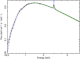
We start with an “average” but high signal-to-noise ratio source modelled with an intrinsically absorbed powerlaw and an unresolved Gaussian line at 6.4 keV, with the average values of the full sample (see Table 1): $z=1.15$, $\Gamma=1.24$, $N_{\rm H}=1.75\times 10^{22}$ cm^-2, EW=100 eV. We compared the input model with the response-matrix-corrected spectra (“unfolded” spectra in XSPEC) assuming three different models:

1. the input model without the Gaussian

2. a powerlaw with $\Gamma=0$

3. a powerlaw with $\Gamma=2$.

We can see the results in Figs. 21 in the observed frame. The best approximation is obtained using the input parameters, as expected. However, in a wide range around the line, the result does not depend noticeably on the model used for the response matrix correction, even for models clearly different from the input one. The significant discrepancies start only below about 2 keV rest-frame.

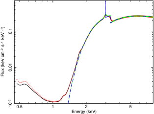
We ran another simulation for an absorbed source, using the continuum parameters of one source in the absorbed subsample, ($z=1.15$, $\Gamma=1.64$; $N_{\rm H}=43.22\times 10^{22}$ cm^-2, ) and a Gaussian at 6.4 keV with $\sigma=0$, EW = 100 eV, again with high signal-to-noise ratio. We show in Fig. 22 the input model and the “unfolded” spectra using the three models above. In this case we also see that there is no important difference in the continuum close to the Fe line between the various models. The differences below $\sim$3 keV rest-frame are much stronger in this case compared to the “average” source, but again the result of the input model follows very closely the input spectrum.

Therefore, we chose to correct the spectra for the response matrices using their own best-fit continuum models and we did not simply divide the spectra for the effective area of the detector. This simple method, actually assumes a flat continuum and does not account for the limited spectral resolution of X-ray detectors.

It is important to notice that in any case there is an energy blending that widens the Fe line. We have quantified this effect using simulations, as explained in Sect. 3.3.

Figure 21: Comparison, for a simulated “average” source, between unfolded spectrum with best fit (green circles), with gamma =2 (red plus), with gamma =0 (continuous black line), with model (dashed blue line).

Figure 22: Comparison, for a simulated absorbed source, between: unfolded spectrum with best fit (green circles), with gamma =2 (red plus), with gamma =0 (continuous black line), with model (dashed blue line). The unfolded spectrum obtained with the best fit is along the model, with the exception of the Fe line region, where it deviates.

In order to check the effect of the correction for detector response on the average spectrum, we corrected the spectra for the detector responses using a powerlaw with $\Gamma=2$. We then made the average of the observed and simulated spectra, using the same procedure explained in the Sect. 3. We can see in Fig. 23 the results: the differences are again small and, in any case, within the mutual error bars. If anything, using the best-fit model for the “unfolding” appears to produce a more conservative estimate of the Fe line flux.

Figure 23: Comparison between the average spectra after having corrected for the detector response using: the best fit (average observed spectrum represented by full circles, simulated spectrum by a dashed line) and with the powerlaw with $\mathrm{\Gamma}=2$ (average observed spectrum represented by stars, simulated spectrum by a contiuous line). Sample with the sources with more than 200 net counts.

References

- Alexander et al. (2003) Alexander D. M., Bauer F. E., Brandt W. N. et al., 2003, AJ, 126, 539(A03)
- Alexander et al. (2011) Alexander D.M., Bauer F.E., Brandt W.N. et al., 2011, arXiv:1106.1443v1/
- Arnaud, (1996) Arnaud K.A., 1996, Astronomical Data Analysis Software and System V, eds. Jacoby G. and Barnes J., p17, ASP Conf. Series volume 101
- (4) Arnaud K.A., http://heasarc.gsfc.nasa.gov/docs/xanadu/xspec/wstat.ps
- Bardeen at al. (1972) Bardeen J. M.; Press, W. H.; Teukolsky, S. A., 1972, ApJ, 178, 347-370
- Bianchi et al. (2007) Bianchi S., Guainazzi M., Matt G. & Fonseca Bonilla N. , 2007, A&A, 467, L19
- Braito et al. (2007) Braito V., Reeves J. N., Dewangan G. C. et al., 2008, ApJ, 670, 978
- Broos et al. (2010) Broos P. S., Townsley L. K., Feigelson E. D. et al. , 2010, ApJ, 714, 1582
- Brusa et al. (2005) Brusa M., Gilli R. & Comastri A., 2005, ApJ, 621, L5
- Brusa et al. (2007) Brusa M., Civano F., Comastri A. & Gilli R., 2007, ASP Conference Series, 380, 167
- Chaudhary et al. (2010) Chaudhary P., Brusa M., Hasinger G., Merloni A. & Comastri A., 2010, A&A, 518, A58
- Corral et al. (2008) Corral A., Page M. J., Carrera F. J. et al., 2008, A&A, 492, 71
- Corral et al. (2011) Corral A., Della Ceca R., Caccianiga A., et al. 2011,A&A, 530, A42
- Digby-North, (2011) Digby-North J., 2011, Investigating the Relationship between Environment and Active Galactic Nuclei Activity at High Redshift, Thesis (PhD), Imperial College London
- Fabian et al. (2000) Fabian A. C., Iwasawa K., Reynolds C.S., Young A.J., 2000, PASP, Volume 112, Issue 775, pp. 1145-1161
- Fabian et al. (2002) Fabian A.C., Vaughan S., Nandra K. et al., 2002, PASP, 335, L1
- George & Fabian (1991) George I.M., Fabian A. C., 1991, MNRAS, 249, March 15, 1991, 352
- Ghisellini et al. (1994) Ghisellini G., Haardt F. & Matt G. , 1994, MNRAS, 267, NO. 3/APR1, 743
- Gilli et al. (1999) Gilli R., Comastri A., Brunetti G. & Setti G. , 1999, astro-ph/9902256v1
- Guainazzi et al. (2006) Guainazzi M., Bianchi S. & M. Dovciak M., 2006, Astron. Nachr., 327, 1032
- Haardt et al. (1991) Haardt F. & Maraschi L., 1991, ApJ, 380, L51-L54
- Hamman et al. (2007) Hamann F., Warner C., Dietrich M. & Ferland G., 2007, Astronomical Society of the Pacific Conference Series, Vol 373, The Central Engine of the Active Galactic Nuclei, ed. L.C. Ho & J.-W. Wang, 653
- Iwasawa et al. (1993) Iwasawa K. & Taniguchi Y., 1993, ApJ, 413, L15
- Iwasawa et al. (1996) Iwasawa, K., Fabian, A. C., Reynolds, et al., 1996, MNRAS, 282, Issue 3, 1038
- Iwasawa et al. (2011) Iwasawa K., Mainieri V., Brusa M., et al., 2011, arXiv:1111.2447v1
- Komatsu et al. (2011) Komatsu E., Smith, K. M., Dunkley, J. et al., 2011, ApJS, 192, Issue 2, article id. 18
- Laird et al. (2009) Laird E. S., Nandra K., Georgakakis A. et al., 2009, ApJS, 180, 102
- Luo et al. (2008) Luo B., Bauer F.E., Brandt W. N., et al., 2008, ApJS, Vol. 179, p. 19
- Mateos et al. (2005) Mateos S., Barcons X., Carrera F.J. , et al., 2005, A&A, 433, 855
- Mateos et al. (2010) Mateos S., Carrera F.J., Page M.J., et al., 2010, A&A, 510, A35
- Matt et al. (1991) Matt G., Perola G. C., Piro L., 1991, Proceedings of a Workshop Held in Varenna, Como, Italy, 9-12 October 1990, edited by Aldo Treves, Giulio C. Perola, and Luigi Stella. Springer-Verlag Berlin Heidelberg New York, 385, 201
- Matt et al. (1996) Matt G., Fabian A.C., Ross R.R., 1996, MNRAS, 278, Issue 4, 1111
- Matt et al. (2005) Matt G., Porquet D., Bianchi S., et al., 2005, A&A, 435, Issue 3, 857
- Nandra et al. (2006) Nandra K., O’Neill P. M., George I. M., Reeves J. N., & Turner T. J., 2006, Astron. Nachr., 327, 1039
- Nandra et al. (1997) Nandra K., George I. M., Mushotzky R. F., Turner T.J. & Yaqoob T., 1997, ApJ, 488, L91
- Page et al. (2004) Page K.L., O’Brien P.T., Reeves J.N. & Turner M.J.L., 2004, MNRAS, 347, 316
- Pounds et al. (2001) Pounds K.A. & Reeves J.N., 2001, arXiv:astro-ph/0201436
- Press et al. (2007) Press W.H. ,Teukolsky S. A. , Vetterling V. T. & Flannery B.P., 2007, Numerical Recipes, Cambridge University Press
- Shakura et al. (1974) Shakura N. I. & Sunyaev R. A. , 1974, A&A, 24, 337
- Streblyanska et al. (2005) Streblyanska A., Hasinger G., Barcons X., Mateos S. & Fabian A. C., 2005,A&A, 432, 395
- Xue et al. (2011) Xue Y. Q., Luo B., Brandt W.N., et al., 2011, arXiv:1105.5643v1
- Yaqoob (2006) Yaqoob T., 2006, IAUS, 230, 461
- Yaqoob (2007) Yaqoob T., 2007, ASP Conference Series, Vol. 373, proceedings of the conference held 16-21 October, 2006 at Xi’an Jioatong University, Xi’an, China. Edited by Luis C. Ho and Jian-Min Wang, 109