Bounded Domain Problem for the Modified Buckley-Leverett Equation
Abstract.
The focus of the present study is the modified Buckley-Leverett (MBL) equation describing two-phase flow in porous media. The MBL equation differs from the classical Buckley-Leverett (BL) equation by including a balanced diffusive-dispersive combination. The dispersive term is a third order mixed derivatives term, which models the dynamic effects in the pressure difference between the two phases. The classical BL equation gives a monotone water saturation profile for any Riemann problem; on the contrast, when the dispersive parameter is large enough, the MBL equation delivers non-monotone water saturation profile for certain Riemann problems as suggested by the experimental observations. In this paper, we first show that the solution of the finite interval boundary value problem converges to that of the half-line boundary value problem for the MBL equation as . This result provides a justification for the use of the finite interval boundary value problem in numerical studies for the half line problem. Furthermore, we extend the classical central schemes for the hyperbolic conservation laws to solve the MBL equation which is of pseudo-parabolic type. Numerical results confirm the existence of non-monotone water saturation profiles consisting of constant states separated by shocks.
Key words and phrases:
conservation laws, dynamic capillarity, two-phase flows, porous media, shock waves, pseudo-parabolic equations, central schemes2000 Mathematics Subject Classification:
35L65, 35L67, 35K70, 76S05, 65M06, 65M081. Introduction
The classical Buckley-Leverett (BL) equation [3] is a simple model for two-phase fluid flow in a porous medium. One application is secondary recovery by water-drive in oil reservoir simulation. In one space dimension the equation has the standard conservation form
| (1.1) | |||||
with the flux function being defined as
| (1.5) |
In this content, denotes the water saturation (e.g. means pure water, and means pure oil), is a constant which indicates water saturation at , and is the water/oil viscosity ratio. The classical BL equation (1.1) is a prototype for conservation laws with convex-concave flux functions. The graph of and with is given in Figure 1.1.
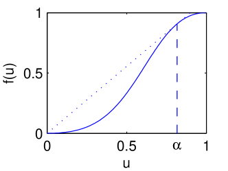
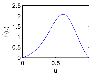
Due to the possibility of the existence of shocks in the solution of the hyperbolic conservation laws (1.1), the weak solutions are sought. The function is called a weak solution of the conservation laws (1.1) if
Notice that the weak solution is not unique. Among the weak solutions, the entropy solution is physically relevant and unique. The weak solution that satisfies Oleinik entropy condition [19]
| (1.6) |
is the entropy solution, where , are the function values to the left and right of the shock respectively, and the shock speed satisfies Rankine-Hugoniot jump condition [17, 10]
| (1.7) |
The classical BL equation (1.1) with flux function as given in (1.5) has been well studied (see [14] for an introduction). Let be the solution of , i.e.,
| (1.8) |
The entropy solution of the classical BL equation can be classified into two categories:
-
(1)
If , the entropy solution has a single shock at .
-
(2)
If , the entropy solution contains a rarefaction between and for and a shock at .
These two types of solutions are shown in Figure 1.2 for .
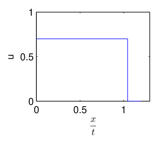
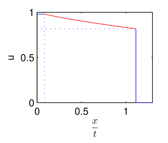
In either case, the entropy solution of the classical BL equation (1.1) is a non-increasing function of at any given time . However, the experiments of two-phase flow in porous medium reveal complex infiltration profiles, which may involve overshoot, i.e., profiles may not be monotone [7]. This suggests the need of modification to the classical BL equation (1.1).
To better describe the infiltration profiles, we go back to the origins of (1.1). Let be the saturation of water/oil () and assume that the medium is completely saturated, i.e. . The conservation of mass gives
| (1.9) |
where is the porosity of the medium (relative volume occupied by the pores) and denotes the discharge of water/oil with , which is assumed to be a constant in space due to the complete saturation assumption. Throughout of this work, we consider it constant in time as well. By Darcy’s law
| (1.10) |
where denotes the absolute permeability, is the relative permeability and is the viscosity of water/oil. Instead of considering constant capillary pressure as adopted by the classical BL equation (1.1), Hassanizadeh and Gray [8, 9] have defined the dynamic capillary pressure as
| (1.11) |
where is the static capillary pressure and is a positive constant, and is the dynamic effects. Using Corey [6, 20] expressions with exponent 2, , rescaling and combining (1.9)-(1.11), the single equation for the water saturation is
| (1.12) |
where [22]. Linearizing the right hand side of (1.12) and rescaling the equation as in [21, 20], the modified Buckley-Leverett equation (MBL) is derived as
| (1.13) |
where the water fractional flow function is given as in (1.5). Notice that, if in (1.11) is taken to be constant, then (1.12) gives the classical BL equation; while if the dispersive parameter is taken to be zero, then (1.13) gives the viscous BL equation, which still displays monotone water saturation profile. Thus, in addition to the classical second order viscous term , the MBL equation (1.13) is an extension involving a third order mixed derivative term . Van Dujin et al. [21] showed that the value is critical in determining the type of the solution profile. In particular, for certain Riemann problems, the solution profile of (1.13) is not monotone when is larger than the threshold value , where was numerically determined to be 0.61 [21]. The non-monotonicity of the solution profile is consistent with the experimental observations [7].
The classical BL equation (1.1) is hyperbolic, and the numerical schemes for hyperbolic equations have been well developed (e.g. [14, 15, 4, 5, 18, 12] ). The MBL equation (1.13), however, is pseudo-parabolic, we will illustrate how to extend the central schemes [18, 12, 13] to solve (1.13) numerically. Unlike the finite domain of dependence for the classical BL equation (1.1), the domain of dependence for the MBL equation (1.13) is infinite. This naturally raises the question for the choice of computational domain. To answer this question, we will first study the MBL equation equipped with two types of domains and corresponding boundary conditions. One is the half line boundary value problem
| (1.14) |
and the other one is finite interval boundary value problem
| (1.15) |
Considering
| (1.16) |
we will show the relation between the solutions of problems (1.14) and (1.15). To the best knowledge of the authors, there is no such study for MBL equation (1.13). Similar questions were answered for BBM equation [1, 2].
The organization of this paper is as follows. Section 2 will bring forward the exact theory comparing the solutions of (1.14) and (1.15). The difference between the solutions of these two types of problems decays exponentially with respect to the length of the interval for practically interesting initial profiles. This provides a theoretical justification for the choice of the computational domain. In section 3, high order central schemes will be developed for MBL equation in finite interval domain. We provide a detailed derivation on how to extend the central schemes [18, 12] for conservation laws to solve the MBL equation (1.13). The idea of adopting numerical schemes originally designed for hyperbolic equations to pseudo-parabolic equations is not restricted to central type schemes only ([23, 24]). The numerical results in section 4 show that the water saturation profile strongly depends on the dispersive parameter value as studied in [21]. For , the MBL equation (1.13) gives non-monotone water saturation profiles for certain Riemann problems as suggested by experimental observations [7]. Section 5 gives the conclusion of the paper and the possible future directions.
2. The half line problem versus the finite interval problem
Let be the solution to the half line problem (1.14), and let be the solution to the finite interval problem (1.15). We consider the natural assumptions (1.16). The goal of this section is to develop an estimate of the difference between and on the spatial interval at a given finite time . The main result of this section is
Theorem 2.1 (The main Theorem).
If satisfies
| (2.1) |
where and are positive constants, then
for some , and , where
Notice that the initial condition (2.1) we considered is the Riemann problem. Theorem 2.1 shows that the solution to the half line problem (1.14) can be approximated as accurately as one wants by the solution to the finite interval problem (1.15) in the sense that , , and can be controlled.
To prove theorem 2.1, we first derive the implicit solution formulae for the half line problem and the finite interval problem in section 2.1 and section 2.2 respectively. The implicit solution formulae are in integral form, which are derived by separating the -derivative from the -derivative, and formally solving a first order linear ODE in and a second order non-homogeneous ODE in . In section 2.3, we use Gronwall’s inequality multiple times to obtain the desired result in theorem 2.1.
2.1. Half line problem
In this section, we derive the implicit solution formula for the half line problem (1.14) (with ). To solve (1.14), we first rewrite (1.14) by separating the -derivative from the -derivative,
| (2.2) |
By using integrating factor method, we formally integrate (2.2) over to obtain
| (2.3) |
Furthermore, we let
| (2.4) |
then (2.3) can be written as
| (2.5) |
Notice that (2.5) is a second-order non-homogeneous ODE in -variable along with the boundary conditions
| (2.6) |
To solve (2.5), we first solve the corresponding linear homogeneous equation with the non-zero boundary conditions (2.6). We then find a particular solution for the non-homogeneous equation with zero boundary conditions by introducing a Green’s function and a kernel for the non-homogeneous terms and respectively. Combining the solutions for the two non-homogeneous terms and the homogeneous part with boundary conditions, we get the solution for equation (2.5) satisfying the boundary conditions (2.6):
| (2.7) |
where the Green’s function and the kernel are
| (2.8) | |||||
| (2.9) |
To recover the solution for the half line problem (1.14), we refer to the definition of in (2.4). Thus, the implicit solution formula for the half line problem (1.14) is
| (2.10) |
2.2. Finite interval problem
The implicit solution for the finite interval problem (1.15) (with ) can be solved in a similar way. The only difference is that the additional boundary condition at in (1.15) gives different boundary conditions for the non-homogeneous ODE in -variable. Denote
| (2.11) |
then it satisfies
| (2.12) |
with the boundary conditions
These boundary conditions affect both the homogeneous solution and the particular solution of (2.12) as follows
| (2.13) |
where the Green’s function , the kernel and the bases for the homogeneous solutions are
| (2.14) |
| (2.15) |
| (2.16) | |||
| (2.17) |
Thus, the implicit solution formula for the finite interval problem (1.15) is
| (2.18) |
2.3. Comparisons
In this section, we will prove that the solution to the half line problem can be approximated as accurately as one wants by the solution to the finite interval problem as stated in Theorem 2.1.
Due to the difference in the integration domains, we do not use (2.10) and (2.18) directly for the comparison. Instead, we decompose ( respectively) into two parts: and ( and respectively), such that ( respectively) enjoys zero initial condition and boundary conditions at and . We estimate the difference between and by estimating the differences between and , and , then applying the triangle inequality.
2.3.1. Definitions and lemmas
To assist the proof of Theorem 2.1 in section 2.3.3, we introduce some new notations in this section. We first decompose as sum of two terms and , such that
where
| (2.19) |
and and are given in (2.16) and (2.17) respectively. With this definition, takes care of the initial condition and boundary conditions at and for . Then satisfies an equation slightly different from the equation satisfies in (1.14):
| (2.20) |
In addition, has zero initial condition and boundary conditions at and , i.e.,
| (2.21) |
Similarly, for , let
where
| (2.22) |
and , and , are given in (2.16) and (2.17) respectively. With this definition, takes care of the initial condition and boundary conditions and at and for . Then satisfies an equation slightly different from the equation satisfies in (1.15):
| (2.23) |
with
| (2.24) |
Since, in the end, we want to study the difference between and , we define
Because of (2.20) and (2.23), we have
| (2.25) |
In lieu of (2.21) and (2.24), also has zero initial condition and boundary conditions at and , i.e.,
| (2.26) |
Now, to estimate , we can estimate and estimate separately. These estimates are done in section 2.3.3.
Next, we state the lemmas needed in the proof of Theorem 2.1. The proof of the lemmas can be found in the appendix A and [22]. In all the lemmas, we assume and satisfies
| (2.29) |
where and are positive constants. Notice that the constraint is crucial in Lemmas 2.3, 2.4.
Lemma 2.2.
where and .
Lemma 2.3.
-
(i)
-
(ii)
.
-
(iii)
.
Lemma 2.4.
-
(i)
.
-
(ii)
.
-
(iii)
.
Lemma 2.5.
-
(i)
.
-
(ii)
for .
-
(iii)
if for .
Last but not least, the norm that we will use in Theorem 2.1 and its proof is
| (2.30) |
2.3.2. A proposition
In this section, we will give a critical estimate, which is essential in the calculation of maximum difference in section 2.3.3. By comparing and given in (2.19) and (2.22) respectively, it is clear that the coefficient for appeared in (2.19) needs to be compared with the corresponding coefficient for appeared in (2.22). We thus define a space-dependent function
| (2.31) |
and establish the following proposition
Proposition 2.6.
| (2.32) |
for some parameter-dependent constants , and .
Proof.
Based on the implicit solution formula (2.10) derived in section 2.1, Lemma 2.2 and the relationship between and given in (2.31), we can get an inequality in terms of
| (2.33) |
To show that decays exponentially with respect to , we pull out an exponential term by writing , where , such that
| (2.34) |
then (2.33) can be rewritten in terms of as follows
| (2.35) |
Because of Lemmas 2.3–2.4, we can get the following estimate for based on (2.35) :
| (2.36) |
where
By Gronwall’s inequality, inequality (2.36) gives that
Hence i.e., decays exponentially with respect to . In particular, when , we have
| (2.37) |
as given in (2.32). ∎
2.3.3. Proof of Theorem 2.1
In this section, we will first find the maximum difference of , then we will derive and . Combining these two, we will get an estimate for .
Proposition 2.7.
Proof.
Proof.
Proposition 2.9.
Proof.
Now we are in the position to prove the main theorem of this section.
Theorem 2.10.
Proof of the Main Theorem.
where
∎
This result gives that exponentially delays in . This theorem shows that if and converge to infinity, then the solution of the finite interval problem converges to the solution of the half line problem in the sense of . This can be achieved either by letting or . For example, in the extreme case, , the half line problem (1.14) becomes hyperbolic and the domain of dependence is finite, so, certainly, one only need to consider the finite interval problem. This is consistent with the main theorem in the sense that for a fixed final time , if and , i.e., , then as . Theorem 2.10 gives a theoretical justification for using the solution of the finite interval problem to approximate the solution of the half line problem with appropriate choice of and . Hence in the next chapter, the numerical scheme designed to solve the MBL equation (1.13) is given for finite interval problem.
3. Numerical schemes
To numerically solve the MBL equation (1.13), We first collect all the terms with time derivative and rewrite MBL equation (1.13) as
| (3.1) |
By letting
| (3.2) |
MBL equation (3.1) can be written as
| (3.3) |
Now, the new form of MBL equation (3.3) can be viewed as a PDE in terms of , and the occurrence of can be recovered by (3.2). Equation (3.3) can be formally viewed as
| (3.4) |
which is a balance law in term of . We adopt numerical schemes originally designed for hyperbolic equations to solve the MBL equation (3.1), which is of pseudo-parabolic type. The local discontinuous Galerkin method has been applied to solve equations involving mixed derivatives term [23, 24]. To the best knowledge of the authors, the central schemes have not been applied to solve equations of this kind. The main advantage of the central schemes is the simplicity. “the direction of the wind“ is not required to be identified, and hence the field-by-field decomposition can be avoided. In this chapter, we demonstrate how to apply the central schemes to solve the MBL equation (3.1).
3.1. Second-order schemes
In this section, we show how to apply the classical second order central schemes [18] originally designed for hyperbolic conservation laws to numerically solve the MBL equation (1.13), which is of pseudo-parabolic type. To solve (3.3), we modify the central scheme given in [18]. As in [18], at each time level, we first reconstruct a piecewise linear approximation of the form
| (3.5) |
Second-order accuracy is guaranteed if the so-called vector of numerical derivative , which will be given later, satisfies
| (3.6) |
We denote the staggered piecewise-constant functions as
| (3.7) |
Evolve the piecewise linear interplant (3.5) by integrating (3.3) over
| (3.8) |
We calculate each term on the right hand side of (3.8) below. For , applying the definition of and given in (3.5) to (3.7), we have that
| (3.9) |
The middle two integrands can be approximated by the midpoint rule
| (3.10) |
if the CFL condition
is met. For MBL equation (3.3), we have that at ,
Let , then
where
Hence the eigenvalues for are
Therefore, the CFL condition is
In the numerical computations in chapter 4, we chose . In (3.10), to estimate ’s, we use Taylor expansion and the conservation law (3.3):
| (3.11) |
where is the discrete central difference operator
and the second-order accuracy is met if
| (3.12) |
The choices for {} in (3.6) and {} in (3.12) can be found in [18], and we chose
| (3.13) |
where and . Combining (3.8)-(3.10), we obtain
| (3.14) |
Next, we will re-write (3.14) in terms of . is approximated as
and using the cell averages, it becomes
| (3.15) |
Notice that the linear interpolation (similar to (3.5))
and the cell average definition (similar to (3.7))
ensure that
and the convertion between and is done using the following relation
| (3.16) |
Hence re-writting (3.14) in terms of gives the staggered central scheme
| (3.17) |
We will focus on the last integral in (3.17). There are many ways to numerically calculate this integral. We will show two ways to do this in the following two subsections, both of them achieve second order accuracy.
3.1.1. Trapezoid Scheme
3.1.2. Midpoint Scheme
3.2. A third order semi-discrete scheme
Similarly, we can extend the third order scheme to solve MBL equation (1.13), however, it is more involved. But the third order semi-discrete central scheme proposed in [12] can be extended to solve the MBL equation in a straightforward manner. In order to make the paper self-contained, we include the formulation below.
where denotes the cell average of
is the numerical convection flux and is a high-order approximation to the diffusion term .
where denote the left and right intermediate values of at , and their values are converted from the using (3.2). The way to calculate , and is
where
The diffusion is approximated using the following fourth-order central differencing form
| (3.23) |
The unique feature of this scheme is that the discretization is done in space first, and then the time evolution equation can be solved as a system of ordinary differential equations using any ODE solver of third order or higher. In this paper, we simply use the standard fourth order Runge-Kutta methods. Notice that to achieve the third order accuracy, the linear solver that converts from using (3.2) need also to be high order, and (3.23) is used to discretize in our convertion.
4. Computational results
In this section, we show the numerical solutions to the MBL equation
| (4.1) |
with the initial condition
| (4.4) |
and the Dirichlet boundary condition.
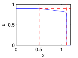
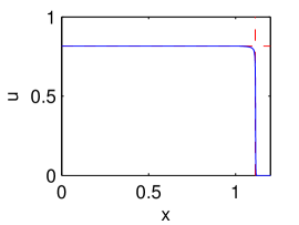
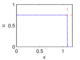
Numerically, it is not practical to solve the half line problem (4.4), and one has to choose an appropriate computational domain. Theorem 2.10 in Chapter 2 provides a theoretical bound for the difference between the solution to the half line problem and that to the finite interval problem. However, the estimate (2.44) in Theorem 2.10 includes time-dependent parameters and , which cannot be obtained analyticaly. Therefore, we numerically demonstrate how the computational domain size affects the solution. We choose , and as an example here. Figure 4.1 shows the snapshot of the solutions at , and for computational domain with , and .
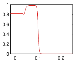
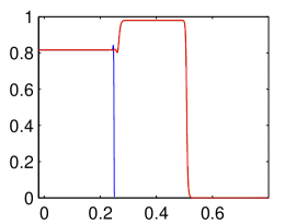
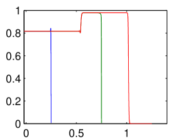
In Figure 4.11(a), , the leading shock is located at , and , , all exceed the leading shock location. Hence all the three computational domains deliver visually indistinguishable results. Whereas, in Figure 4.11(b), , the leading shock is located at , is shorter than the computational domain needed to capture this shock, hence the numerical solution halts at . On the contrast, and are both large enough to capture this shock front. Similarly, in Figure 4.11(c), , the leading shock is located at 1.02. and both result in wrong solution profiles. More specifically, both solutions halt at the boundary of the insufficient computational domain. But is large enough to capture the correct solution profile.
In the rest of this chapter, all the computational domains are therefore chosen based on the principle:
In addition, numerical solutions for larger ’s, for example, , , , are also sought. For all these larger ’s, the numerical solutions are all consistent with that corresponding to up to . This confirms that it is not necessary to take too much larger than leading shock speed computational time.
To validate the order analysis given in chapter 3 for various schemes proposed, we first test the order of our schemes numerically with a smooth initial condition
where
The final time was employed, so that there was no shock created. in the MBL equation (4.1) is taken to be 1, is taken to be 2, and the computational interval is . The order tests of the trapezoid scheme and the third order semi-discrete scheme with different parameter value and the initial condition are given in Tables 4.1, 4.2. Table 4.1 shows that the trapezoid rule achieved second order accuracy for all the tested cases in sense. Table 4.2 shows that the semi-discrete scheme has the order of accuracy greater than 2.5 for all the cases, and exceeds 3 for some cases. This confirms the accuracy study given in sections 3.1.1 and 3.2 respectively.
| N | order | order | order | ||||
|---|---|---|---|---|---|---|---|
| 60 | 7.5416e-03 | - | 2.5388e-03 | - | 1.5960e-03 | - | |
| 120 | 1.9684e-03 | 1.9379 | 6.7288e-04 | 1.9157 | 4.4066e-04 | 1.8568 | |
| 240 | 4.9891e-04 | 1.9802 | 1.7645e-04 | 1.9311 | 1.2529e-04 | 1.8144 | |
| 480 | 1.2589e-04 | 1.9865 | 4.5366e-05 | 1.9596 | 3.3205e-05 | 1.9158 | |
| 60 | 8.0141e-03 | - | 2.6069e-03 | - | 1.4989e-03 | - | |
| 120 | 2.1502e-03 | 1.8981 | 7.0452e-04 | 1.8876 | 4.2221e-04 | 1.8279 | |
| 240 | 5.5697e-04 | 1.9488 | 1.8259e-04 | 1.9480 | 1.1283e-04 | 1.9038 | |
| 480 | 1.4104e-04 | 1.9815 | 4.6109e-05 | 1.9855 | 2.8719e-05 | 1.9740 | |
| 60 | 1.3102e-02 | - | 4.1784e-03 | - | 2.2411e-03 | - | |
| 120 | 3.6201e-03 | 1.8557 | 1.0994e-03 | 1.9263 | 6.1060e-04 | 1.8759 | |
| 240 | 9.6737e-04 | 1.9039 | 2.8089e-04 | 1.9686 | 1.5667e-04 | 1.9625 | |
| 480 | 2.5825e-04 | 1.9053 | 7.1250e-05 | 1.9790 | 3.9286e-05 | 1.9956 | |
| 60 | 6.4427e-03 | - | 2.1578e-03 | - | 1.1682e-03 | - | |
| 120 | 1.6611e-03 | 1.9555 | 5.7775e-04 | 1.9011 | 3.6447e-04 | 1.6804 | |
| 240 | 4.3643e-04 | 1.9283 | 1.5215e-04 | 1.9250 | 1.0389e-04 | 1.8107 | |
| 480 | 1.1223e-04 | 1.9593 | 3.9170e-05 | 1.9577 | 2.7629e-05 | 1.9109 | |
| 60 | 7.5867e-03 | - | 2.4101e-03 | - | 1.3364e-03 | - | |
| 120 | 2.0069e-03 | 1.9185 | 6.4998e-04 | 1.8906 | 3.7650e-04 | 1.8277 | |
| 240 | 5.1832e-04 | 1.9531 | 1.6801e-04 | 1.9519 | 1.0062e-04 | 1.9037 | |
| 480 | 1.3136e-04 | 1.9803 | 4.2497e-05 | 1.9831 | 2.5599e-05 | 1.9748 | |
| 60 | 1.1959e-02 | - | 3.8026e-03 | - | 1.9938e-03 | - | |
| 120 | 3.2940e-03 | 1.8602 | 9.9527e-04 | 1.9338 | 5.4231e-04 | 1.8783 | |
| 240 | 8.7736e-04 | 1.9086 | 2.5358e-04 | 1.9727 | 1.3933e-04 | 1.9606 | |
| 480 | 2.3271e-04 | 1.9146 | 6.4252e-05 | 1.9806 | 3.4967e-05 | 1.9944 | |
| 60 | 5.7714e-03 | - | 1.9358e-03 | - | 1.0481e-03 | - | |
| 120 | 1.5035e-03 | 1.9406 | 5.1617e-04 | 1.9070 | 2.8061e-04 | 1.9011 | |
| 240 | 3.9299e-04 | 1.9357 | 1.3616e-04 | 1.9225 | 7.9134e-05 | 1.8262 | |
| 480 | 1.0063e-04 | 1.9655 | 3.5080e-05 | 1.9566 | 2.1035e-05 | 1.9115 | |
| 60 | 7.1823e-03 | - | 2.2843e-03 | - | 1.2069e-03 | - | |
| 120 | 1.8963e-03 | 1.9213 | 6.1315e-04 | 1.8974 | 3.4013e-03 | 1.8272 | |
| 240 | 4.8284e-04 | 1.9736 | 1.5796e-04 | 1.9567 | 9.0912e-04 | 1.9035 | |
| 480 | 1.2093e-04 | 1.9974 | 3.9783e-05 | 1.9894 | 2.3121e-05 | 1.9753 | |
| 60 | 1.1042e-02 | - | 3.5020e-03 | - | 1.8299e-03 | - | |
| 120 | 3.0287e-03 | 1.8662 | 9.1181e-04 | 1.9414 | 4.8976e-04 | 1.9016 | |
| 240 | 8.0111e-04 | 1.9186 | 2.3118e-04 | 1.9797 | 1.2593e-04 | 1.9595 | |
| 480 | 2.1076e-04 | 1.9264 | 5.8358e-05 | 1.9860 | 3.1627e-05 | 1.9934 |
| order | order | order | |||||
|---|---|---|---|---|---|---|---|
| 120 | 2.6992e-03 | - | 1.1300e-03 | - | 7.2363e-04 | - | |
| 240 | 4.0403e-04 | 2.7400 | 1.7079e-04 | 2.7260 | 1.1283e-04 | 2.6811 | |
| 480 | 5.7504e-05 | 2.8127 | 2.4624e-05 | 2.7941 | 1.6242e-05 | 2.7963 | |
| 960 | 8.4934e-06 | 2.7592 | 3.0892e-06 | 2.9948 | 1.7607e-06 | 3.2055 | |
| 120 | 4.7731e-03 | - | 2.0192e-03 | - | 1.7267e-03 | - | |
| 240 | 8.7205e-04 | 2.4524 | 3.6879e-04 | 2.4529 | 3.0632e-04 | 2.4949 | |
| 480 | 1.2006e-04 | 2.8606 | 5.0480e-05 | 2.8690 | 4.1985e-05 | 2.8671 | |
| 960 | 1.5942e-05 | 2.9129 | 6.6663e-06 | 2.9208 | 5.1464e-06 | 3.0282 | |
| 120 | 3.7573e-03 | - | 1.2122e-03 | - | 7.9211e-04 | - | |
| 240 | 7.4624e-04 | 2.3320 | 2.4164e-04 | 2.3267 | 1.5061e-04 | 2.3949 | |
| 480 | 1.1994e-04 | 2.6373 | 3.8434e-05 | 2.6524 | 2.5089e-05 | 2.5857 | |
| 960 | 1.5565e-05 | 2.9460 | 4.9190e-06 | 2.9660 | 3.1363e-06 | 2.9999 | |
| 120 | 2.1836e-03 | - | 9.1039e-04 | - | 5.7219e-04 | - | |
| 240 | 3.2729e-04 | 2.7381 | 1.3760e-04 | 2.7260 | 8.9550e-05 | 2.6757 | |
| 480 | 4.6856e-05 | 2.8043 | 1.9909e-05 | 2.7890 | 1.2935e-05 | 2.7914 | |
| 960 | 6.7382e-06 | 2.7978 | 2.3182e-06 | 3.1023 | 1.4109e-06 | 3.1965 | |
| 120 | 3.9014e-03 | - | 1.6388e-03 | - | 1.3873e-03 | - | |
| 240 | 7.0517e-04 | 2.4680 | 2.9669e-04 | 2.4656 | 2.4272e-04 | 2.5149 | |
| 480 | 9.6528e-05 | 2.8690 | 4.0354e-05 | 2.8781 | 3.3125e-05 | 2.8733 | |
| 960 | 1.2890e-05 | 2.9047 | 5.3648e-06 | 2.9111 | 4.0754e-06 | 3.0229 | |
| 120 | 3.0797e-03 | - | 9.9202e-04 | - | 6.4456e-04 | - | |
| 240 | 6.1133e-04 | 2.3328 | 1.9783e-04 | 2.3261 | 1.2277e-04 | 2.3924 | |
| 480 | 9.7351e-05 | 2.6507 | 3.1222e-05 | 2.6637 | 2.0263e-05 | 2.5990 | |
| 960 | 1.2396e-05 | 2.9733 | 3.9513e-06 | 2.9822 | 2.4962e-06 | 3.0210 | |
| 120 | 1.8244e-03 | - | 7.5548e-04 | - | 4.6671e-04 | - | |
| 240 | 2.7262e-04 | 2.7425 | 1.1419e-04 | 2.7260 | 7.3299e-05 | 2.6707 | |
| 480 | 3.9198e-05 | 2.7980 | 1.6562e-05 | 2.7855 | 1.0681e-05 | 2.7788 | |
| 960 | 5.4739e-06 | 2.8401 | 1.9677e-06 | 3.0733 | 1.3232e-06 | 3.0129 | |
| 120 | 3.2727e-03 | - | 1.3672e-03 | - | 1.1477e-03 | - | |
| 240 | 5.8671e-04 | 2.4798 | 2.4585e-04 | 2.4754 | 1.9866e-04 | 2.5304 | |
| 480 | 7.9974e-05 | 2.8750 | 3.3285e-05 | 2.8848 | 2.7033e-05 | 2.8775 | |
| 960 | 1.0724e-05 | 2.8987 | 4.4466e-06 | 2.9041 | 3.3341e-06 | 3.0193 | |
| 120 | 2.5902e-03 | - | 8.3335e-04 | - | 5.3882e-04 | - | |
| 240 | 5.1342e-04 | 2.3348 | 1.6611e-04 | 2.3268 | 1.0271e-04 | 2.3913 | |
| 480 | 8.1062e-05 | 2.6630 | 2.6032e-05 | 2.6738 | 1.6813e-05 | 2.6109 | |
| 960 | 1.0173e-05 | 2.9944 | 3.2662e-06 | 2.9946 | 2.0473e-06 | 3.0377 |
We will now use examples to study the solutions to MBL equation (4.1) using the numerical schemes proposed in chapter 3. We first notice that if we scale and as follows
then MBL (4.1) equation can be written in terms of and as follows
| (4.6) |
The scaled equation (4.6) shows that it is the magnitude of and that determine the asymptotic behavior, not , , neither alone ([21]). In addition, (4.6) also shows that the dispersive parameter denotes the relative importance of the dispersive term . The bigger is, the more dispersive effect (4.1) equation has. This can be seen from the computational results to be shown later in this section.
Duijn et al. [21] numerically provided a bifurcation diagram (Figure 4.2) of MBL (4.1) equation as the dispersive parameter and the post-shock value of the initial condition vary. The solution of (4.1) has been proven to display qualitatively different profiles for parameter values () falling in different regimes of the bifurcation diagram.
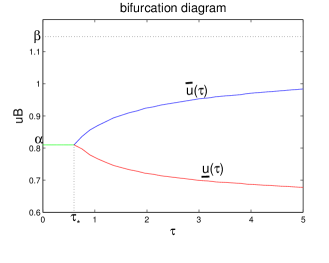
In particular, for every fixed value, there are two critical values, namely, and . From the bifurcation diagram (Figure 4.2), it is clear that, when , . For a fixed value, the solution has three different profiles.
-
(a)
If , the solution contains a plateau value for , a rarefaction wave connection to for , another plateau value for , and a shock from down to at (see Figure 4.3).
-
(b)
If , the solution contains a plateau value for , a shock from up to at , another plateau value for , and a shock from down to at (see Figure 4.3). The solution may exhibit a damped oscillation near .
-
(c)
If , the solution consists a single shock connecting and at (see Figure 4.3). It may exhibit oscillatory behavior near .
Notice that when and , the solution profiles (4.3) displays non-monotonicity, which is consistent with the experimental observations ([7]).
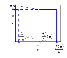
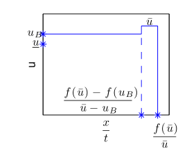
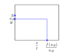
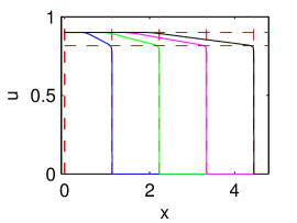
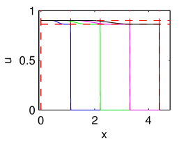
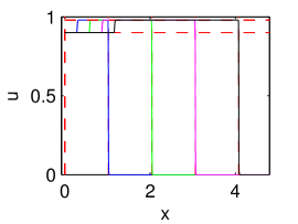
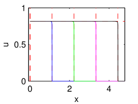
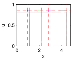
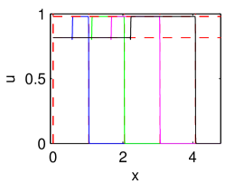
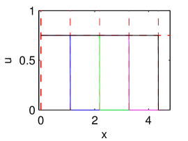
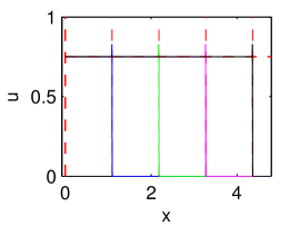
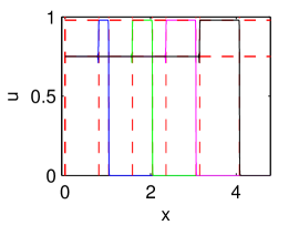
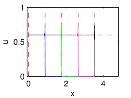
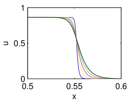
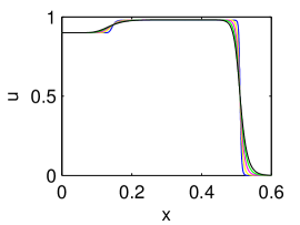
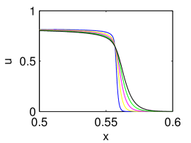
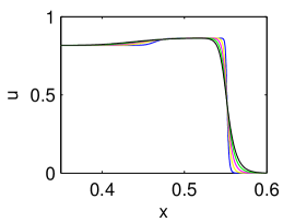
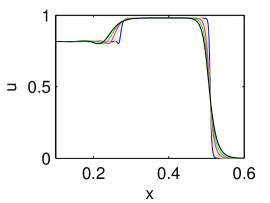
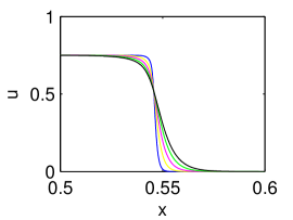
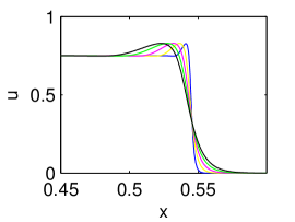
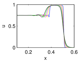
In the numerical computation we show below, we will therefore test the accuracy and capability of central schemes for different parameter values ( and ) that fall into various regimes of the bifurcation diagram, and therefore display qualitatively different solution profiles. The numerical experiments were carried out for , and , i.e. to get the asymptotic solution profiles, and was chosen to be and was chosen to be 0.1. The scheme used in the computation is the second order Trapezoid scheme as shown in section 3.1.1. The Midpoint scheme delivers similar computational results, hence is omitted here. The solution profiles at (blue), (green), (magenta) and (black) are chosen to demonstrate the time evolution of the solutions. The red dashed lines are used to denote the theoretical shock locations and plateau values for comparison purpose.
We start with . Based on the bifurcation diagram (Figure 4.2), we choose three representative values, i.e. , (for ) and . For each fixed , we choose three representative values, i.e. , with , and with . We first use this 9 pairs of values given in Table 4.3 to validate the solution profiles with the demonstrative solution profiles given in Figure 4.3.
| Example 4 | Example 5 | Example 6 | |
|---|---|---|---|
| Example 1 | |||
| Example 2 | |||
| Example 3 |
Example 1 .
When is fixed, we increase from 0.2 to 1 to 5 (Figure 4(a) , 4(b) , 4(c)), the dispersive effect starts to dominate the solution profile. When (Figure 4(a)), the solution profile is similar to the classical BL equation solution (see Figure 2(b)), with a rarefaction wave for and a shock from to at .
This corresponds to Figure 4.3 with .
When (Figure 4(b)), the rarefaction wave is between and the solution remains at the plateau value for and the shock occurs at .
This corresponds to Figure 4.3 with .
When (Figure 4(c)), the solution displays the first shock from to at , and then remains at the plateau value for and the second shocks occurs at .
This corresponds to Figure 4.3 with . Notice that as increases, the rarefaction region shrinks and the plateau region enlarges.
Example 2 .
When is fixed, we increase from 0.2 to 1 to 5 (Figure 4(d) , 4(e) , 4(f)), the dispersive effect starts to dominate the solution profile. When , the solution displays one single shock at . For both and , the solution has two shocks, one at , and another one at . For both and (Figures 4(e) 4(f)), the solutions correspond to Figure 4.3, which are consistent to the experimental observations. Notice that as increases from 1 to 5, i.e., the dispersive effect increases, the inter-shock interval length increases at every fixed time (compare Figure 4(e) with Figure 4(f)). In addition, for fix ( respectively), as time progresses, the inter-shock interval length increases in the linear fashion (see Figure 4(e) (Figure 4(f) respectively) ).
Example 3 .
When is fixed, we increase from 0.2 to 1 to 5 (Figure 4(g) , 4(h) , 4(i)), the dispersive effects starts to dominate the solution profile in the similar fashion as and . Notice that when , since is very close to , the solution displays oscillation at (Figure 4(h)). If we increase further to , the dispersive effect is strong enough to create a plateau value at (see Figure 4(i)).
Example 4 .
Now, we fix , decrease from 0.9 to , to 0.75
(Figures4(a) 4(d) 4(g)). If the solution consists a rarefaction wave connecting down to , then a shock from to 0, otherwise, the solution consists a single shock from down to 0. In all cases, since , regardless of the value, the solution will not display non-monotone behavior, due to the lack of dispersive effect.
Example 5 .
Now, we fix , decrease from 0.9 to , to 0.75 (Figures4(b) 4(e) 4(h)). If , the solution consists a rarefaction wave connecting and , and a shock connecting down to 0 (Figure 4(b)). Even if , because , the solution still has a chance to increase to the plateau value as seen in Figure 4(e). But, if is too small, for example, , the solution does not increase to any more, instead, it consists a single shock connecting down to 0 (Figure 4(h)).
Example 6 .
Now, we fix , decrease from 0.9 to , to 0.75 (Figures4(c) 4(f) 4(i)).
For all three , they are between and , hence all increase to the plateau value before dropping to 0. Notice that as decreases, the inter-shock interval length decreases at every fixed time (compare Figures 4(c), 4(f) and 4(i)). This shows that when the dispersive effect is strong (), the bigger is, the bigger region the solution stays at the plateau value.
Example 7 .
We now show the solution profiles for the extreme value, i.e. in Figures
5(a) (), 5(b) () and 5(c) (). Notice that these are cases of
classical BL equation with small diffusion . We compare Figures
5(a), 5(b) and 5(c) with the
solution of the classical BL equation given in Figures 2(a) and 2(b), it is clear that they show
qualitatively same solution profiles. The difference is that due to the
diffusion term in the MBL equation, as shown in Figure 4.5, the
solutions do not have sharp edges right at the shock, instead, the solutions
smear out a little.
If we compare Figures 5(a), 5(b) and
5(c) with Figures 4(a),
4(d) and 4(g), there is no visible difference. This shows
that once , solution profile will stay the same for a fixed value.
Example 8 .
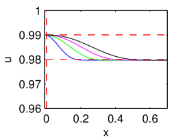
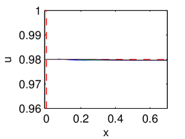
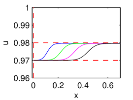
We also study the solution profiles for close to . For example, when , , we hence choose , , and solutions are shown in Figure 6(a), 6(b), 6(c).
If , the solution drops to the plateau value , then drops to 0 (see Figure 6(a)). If , the solution remains at plateau value and then drop to 0 (see Figure 6(b)). If , the solution increases to the plateau value , then drops to 0. In all cases, the transition from to takes very small space. In the majority space, the solution keeps to be the plateau value .
Example 9 , , , , .
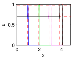
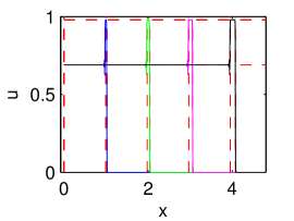
In addition, we study the solution profiles for close to . For example, when
, , we hence choose , , , , and solutions are shown in Figures 7(a), 7(b), 7(c), 7(d), 7(e). As decreases crossing , the solution gradually stops increasing to the plateau value , and the inter-shock interval length decreases (compare Figures 7(a), 7(b) and 7(c)). The oscillation in Figures 7(d) and 7(e) are due to the fact that values are too close to . This confirms that even with big dispersive effect (say ), if is too small (e.g. ), the solution will not exhibit non-monotone behavior.
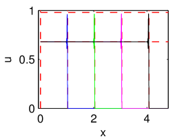
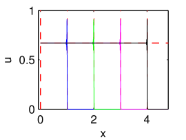
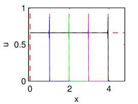
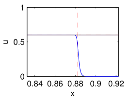
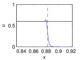
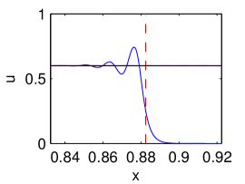
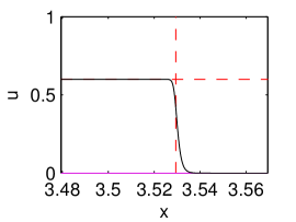
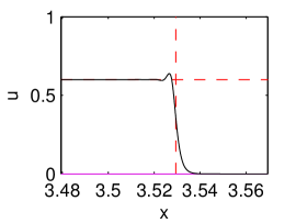
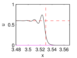
Example 10 , , .
We fix to be small, and in this example, we take it to be . We vary the value, from to barely larger than to . The numerical solutions are given in
Figure 8(a), 8(b), 8(c). As increases, the post-shock
value remains the same, but there will be oscillation generated as becomes larger than . Figures
8(d), 8(e) and 8(f) show that as
increases, the oscillation amplitude increases and oscillates more rounds.
Notice that is the dispersive parameter, and this means that even for small value, different
dispersive parameter values still give different dispersive effects, although none can bring the solution to the
plateau value .
Comparing
Figures 8(d), 8(e) and 8(f) with
Figures 8(g), 8(h) and 8(i), it is clear that
the oscillation amplitude remains steady with respect to time.

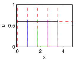
Example 11 .
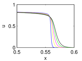
In this example, we will compare the solution profiles for different values. Fixing , we show the numerical results in Figure 4.9
for (blue), (yellow), (magenta), (green),
and (black).
For the purpose of cross reference, we choose the same nine sets of parameter settings as in examples 1– 6. To
assist the observation, the figures in Figure 4.9 are zoomed into the regions where different
values introduce different solution profiles.
The numerical solutions clearly show that as increases, the numerical solution is smeared out, and the
jump location becomes less accurate.
Notice that is responsible for the competition between the diffusion and dispersion, which in turn
determines the plateau values. Hence varying value doesn’t affect the plateau location.
5. Conclusion
We proved that the solution to the infinite domain problem can be approximated by that of the bounded domain problem. This provides a theoretical justification for using finite domain to calculation the numerical solution of the MBL equation (1.13). We also extended the classical central scheme originally designed for the hyperbolic systems to solve the MBL equation, which is of pseudo-parabolic type. The numerical solutions for qualitatively different parameter values and initial conditions show that the jump locations are consistent with the theoretical calculation and the plateau heights are consistent with the numerically obtained values given in [21]. In particular, when , for , the numerical solutions give non-monotone water saturation profiles, which is consistent with the experimental observations. In addition, the order tests show that the proposed second and third order central schemes achieved the desired accuracies.
In [22, 20], the two-dimensional space extension of the modified Buckley-Leverett equation has been derived. One of the future directions is to develop high order numerical schemes to solve the two-dimensional MBL equation. Central schemes have been used to solve high dimensional hyperbolic problem and dispersive problem ([11, 16]), which makes it a good candidate for such a task.
Appendix A Proof of the lemmas
Proof to lemma 2.2.
Let , then
and hence achieves its maximum at . Therefore, , where and , and in turn, we have that for all . ∎
Proof to lemma 2.3 (iii).
Based on the assumption on in (2.29)
| (A.2) |
Calculating with the assumption that , we get
Therefore, we get the desired inequality
∎
Acknowledgments
CYK would like to thank Prof. L.A. Peletier for introducing MBL equation and Mathematical Biosciences Institute at OSU for the hospitality and support.
References
- [1] J. L. Bona, H.-Q. Chen, S. M. Sun, and B.-Y. Zhang, Comparison of quarter-plane and two-point boundary value problems: the BBM-equation, Discrete Contin. Dyn. Syst. 13 (2005), no. 4, 921–940. MR MR2166711 (2006m:35314)
- [2] J. L. Bona and L.-H. Luo, Initial-boundary value problems for model equations for the propagation of long waves, Evolution equations (Baton Rouge, LA, 1992), Lecture Notes in Pure and Appl. Math., vol. 168, Dekker, New York, 1995, pp. 63, 65–94. MR MR1300420 (95i:35137)
- [3] S.E. Buckley and M.C. Leverett, Mechanism of fluid displacement in sands, Petroleum Transactions, AIME 146 (1942), 107–116.
- [4] B. Cockburn, C. Johnson, C.-W. Shu, and E. Tadmor, Advanced numerical approximation of nonlinear hyperbolic equations, Lecture Notes in Mathematics, vol. 1697, Springer-Verlag, Berlin, 1998, Papers from the C.I.M.E. Summer School held in Cetraro, June 23–28, 1997, Edited by Alfio Quarteroni, Fondazione C.I.M.E.. [C.I.M.E. Foundation]. MR MR1729305 (2000h:65004)
- [5] B. Cockburn, G. E. Karniadakis, and C-W (Eds.) Shu, Discontinuous galerkin methods: Theory, computation and applications, Lecture Notes in Computational Science and Engineering, 2000.
- [6] A.T. Corey, The interrelation between gas and oil relative permeabilities, Producer’s Monthly 19 (1954), no. 1, 38–41.
- [7] D. A. DiCarlo, Experimental measurements of saturation overshoot on infiltration, Water Resources Research 40 (2004), 4215.1 – 4215.9.
- [8] S.M Hassanizadeh and W.G. Gray, Mechanics and thermodynamics of multiphase flow in porous media including interphase boundaries, Adv. Water Resour. 13 (1990), 169–186.
- [9] by same author, Thermodynamic basis of capillary pressure in porous media, Water Resour. Res. 29 (1993), 3389–3405.
- [10] H. Hugoniot, Propagation des Mouvements dans les Corps et specialement dans les Gaz Parfaits (in French), Journal de l’Ecole Polytechnique 57 (1887), 3–97.
- [11] G-S Jiang and E. Tadmor, Nonoscillatory central schemes for multidimensional hyperbolic conservation laws, SIAM J. Sci. Comput. 19 (1998), no. 6, 1892–1917 (electronic). MR 1638064 (99f:65128)
- [12] A. Kurganov and D. Levy, A third-order semidiscrete central scheme for conservation laws and convection-diffusion equations, SIAM J. Sci. Comput. 22 (2000), no. 4, 1461–1488 (electronic). MR MR1797891 (2001j:65127)
- [13] A. Kurganov and C.-T. Lin, On the reduction of numerical dissipation in central-upwind schemes, Commun. Comput. Phys. 2 (2007), no. 1, 141–163. MR MR2305919 (2007k:35320)
- [14] R. J. LeVeque, Numerical methods for conservation laws, second ed., Lectures in Mathematics ETH Zürich, Birkhäuser Verlag, Basel, 1992. MR MR1153252 (92m:65106)
- [15] by same author, Finite volume methods for hyperbolic problems, Cambridge Texts in Applied Mathematics, Cambridge University Press, Cambridge, 2002. MR MR1925043 (2003h:65001)
- [16] D. Levy, G. Puppo, and G. Russo, Compact central WENO schemes for multidimensional conservation laws, SIAM J. Sci. Comput. 22 (2000), no. 2, 656–672. MR 1780619 (2001d:65110)
- [17] W. J. Macquorn Rankine, On the thermodynamic theory of waves of finite longitudinal disturbance, Royal Society of London Philosophical Transactions Series I 160 (1870), 277–288.
- [18] H. Nessyahu and E. Tadmor, Nonoscillatory central differencing for hyperbolic conservation laws, J. Comput. Phys. 87 (1990), no. 2, 408–463. MR MR1047564 (91i:65157)
- [19] O. A. Oleĭnik, Discontinuous solutions of non-linear differential equations, Uspehi Mat. Nauk (N.S.) 12 (1957), no. 3(75), 3–73. MR MR0094541 (20 #1055)
- [20] C. J. Van Duijn, A. Mikelic, and I.S. Pop, Effective Buckley-Leverett equations by homogenization, Progress in industrial mathematics at ECMI (2000), 42–52.
- [21] C. J. van Duijn, L. A. Peletier, and I. S. Pop, A new class of entropy solutions of the Buckley-Leverett equation, SIAM J. Math. Anal. 39 (2007), no. 2, 507–536 (electronic). MR MR2338418 (2008g:35136)
- [22] Y. Wang, Central schemes for the modified buckley-leverett equation, Ph.D. thesis, The Ohio State University, 2010.
- [23] Y. Xu and C-W. Shu, A local discontinuous Galerkin method for the Camassa-Holm equation, SIAM J. Numer. Anal. 46 (2008), no. 4, 1998–2021. MR MR2399405 (2009e:65140)
- [24] by same author, Local discontinuous Galerkin method for the Hunter-Saxton equation and its zero-viscosity and zero-dispersion limits, SIAM J. Sci. Comput. 31 (2008/09), no. 2, 1249–1268. MR MR2466156 (2009k:65187)