HPQCD Collaboration

Dβ†’Ο€,lβ€‹Ξ½β†’π·πœ‹π‘™πœˆD\rightarrow\pi,l\nu Semileptonic Decays, |Vc​d|subscript𝑉𝑐𝑑|V_{cd}| and 2nd Row Unitarity from Lattice QCD

Heechang Na Department of Physics, The Ohio State University, Columbus, OH 43210, USA    Christine T.Β H.Β Davies SUPA, School of Physics & Astronomy, University of Glasgow, Glasgow, G12 8QQ, UK    Eduardo Follana Departamento de Fisica Teorica, Universidad de Zaragoza, E-50009 Zaragoza, Spain    Jonna Koponen SUPA, School of Physics & Astronomy, University of Glasgow, Glasgow, G12 8QQ, UK    G.Peter Lepage Laboratory of Elementary Particle Physics, Cornell University, Ithaca, NY 14853, USA    Junko Shigemitsu Department of Physics, The Ohio State University, Columbus, OH 43210, USA
Abstract

We present a new calculation of the Dβ†’Ο€,lβ€‹Ξ½β†’π·πœ‹π‘™πœˆD\rightarrow\pi,l\nu semileptonic form factor f+D→π​(q2)subscriptsuperscriptπ‘“β†’π·πœ‹superscriptπ‘ž2f^{D\rightarrow\pi}_{+}(q^{2}) at q2=0superscriptπ‘ž20q^{2}=0 based on HISQ charm and light valence quarks on MILC Nf=2+1subscript𝑁𝑓21N_{f}=2+1 lattices. Using methods developed recently for HPQCD’s study of Dβ†’K,lβ€‹Ξ½β†’π·πΎπ‘™πœˆD\rightarrow K,l\nu decays, we find f+D→π​(0)=0.666​(29)subscriptsuperscriptπ‘“β†’π·πœ‹00.66629f^{D\rightarrow\pi}_{+}(0)=0.666(29). This signifies a better than factor of two improvement in errors for this quantity compared to previous calculations. Combining the new result with CLEO-c branching fraction data, we extract the CKM matrix element |Vc​d|=0.225​(6)e​x​p.​(10)l​a​t.subscript𝑉𝑐𝑑0.225subscript6𝑒π‘₯𝑝subscript10π‘™π‘Žπ‘‘|V_{cd}|=0.225(6)_{exp.}(10)_{lat.}, where the first error comes from experiment and the second from theory. With a total error of ∼5.3similar-toabsent5.3\sim 5.3% the accuracy of direct determination of |Vc​d|subscript𝑉𝑐𝑑|V_{cd}| from D𝐷D semileptonic decays has become comparable to (and in good agreement with) that from neutrino scattering. We also check for second row unitarity using this new |Vc​d|subscript𝑉𝑐𝑑|V_{cd}|, HPQCD’s earlier |Vc​s|subscript𝑉𝑐𝑠|V_{cs}| and |Vc​b|subscript𝑉𝑐𝑏|V_{cb}| from the Fermilab Lattice & MILC collaborations. We find |Vc​d|2+|Vc​s|2+|Vc​b|2=0.976​(50)superscriptsubscript𝑉𝑐𝑑2superscriptsubscript𝑉𝑐𝑠2superscriptsubscript𝑉𝑐𝑏20.97650|V_{cd}|^{2}+|V_{cs}|^{2}+|V_{cb}|^{2}=0.976(50), improving on the current PDG2010 value.

pacs:
12.38.Gc, 13.20.Fc

I Introduction

The Cabibbo-Kobayashi-Maskawa (CKM) matrix provides particle physicists with a wealth of opportunities to carry out precision tests of the Standard Model (SM) and look for New Physics. On the one hand each matrix element can be determined in several ways, employing different experimental and theory inputs, and the results compared with each other. Three generation unitarity can also be examined to see how well V^C​K​MΓ—V^C​K​M†=I^subscript^𝑉𝐢𝐾𝑀superscriptsubscript^𝑉𝐢𝐾𝑀†^𝐼\hat{V}_{CKM}\times\hat{V}_{CKM}^{\dagger}=\hat{I} is satisfied. This leads to tests such as 1st, 2nd or 3rd row/column unitarity. It also gives rise to the important β€œUnitarity Triangle” relation Vu​dβˆ—Vu​bβˆ—+Vc​dβˆ—Vc​bβˆ—+Vt​dβˆ—Vt​bβˆ—=0subscript𝑉𝑒𝑑subscriptsuperscript𝑉𝑒𝑏subscript𝑉𝑐𝑑subscriptsuperscript𝑉𝑐𝑏subscript𝑉𝑑𝑑subscriptsuperscript𝑉𝑑𝑏0V_{ud}*V^{*}_{ub}+V_{cd}*V^{*}_{cb}+V_{td}*V^{*}_{tb}=0. Consistency checks of the sides and angles of the Unitarity Triangle (UT) have been the focus of much of the experimental and theoretical effort in Flavor Physics in recent years. Lattice QCD is playing an increasingly important role in CKM physics reviews . For instance, lattice calculations of the Kaon semileptonic form factor f+K→π​(0)superscriptsubscriptπ‘“β†’πΎπœ‹0f_{+}^{K\rightarrow\pi}(0) boyle ; lubicz and the decay constant fKsubscript𝑓𝐾f_{K} (or fK/fΟ€subscript𝑓𝐾subscriptπ‘“πœ‹f_{K}/f_{\pi}) milc ; follana ; bmw ; rbc ; etm have contributed to precision determinations of |Vu​s|subscript𝑉𝑒𝑠|V_{us}| and 1st row unitarity tests kaonrev .

The HPQCD collaboration recently published a new lattice calculation of the Dβ†’K,lβ€‹Ξ½β†’π·πΎπ‘™πœˆD\rightarrow K,l\nu semileptonic decay form factor f+Dβ†’K​(q2)subscriptsuperscript𝑓→𝐷𝐾superscriptπ‘ž2f^{D\rightarrow K}_{+}(q^{2}) at q2=0superscriptπ‘ž20q^{2}=0 dtok which significantly reduced the error on this quantity compared to previous theory results. This led to a very precise determination of the CKM matrix element |Vc​s|subscript𝑉𝑐𝑠|V_{cs}|. Features in the HPQCD work that made this improvement possible include the use of a relativistic quark action, the β€œHighly Improved Staggered Quark” (HISQ) action hisq , to simulate both light and charm quarks, better data analysis tools and a new method for carrying out chiral/continuum extrapolations. Capitalizing on these developments, we turn here in this article to Dβ†’Ο€,lβ€‹Ξ½β†’π·πœ‹π‘™πœˆD\rightarrow\pi,l\nu semileptonic decays. We focus on extracting the CKM matrix element |Vc​d|subscript𝑉𝑐𝑑|V_{cd}| by combining theory results for f+D→π​(0)superscriptsubscriptπ‘“β†’π·πœ‹0f_{+}^{D\rightarrow\pi}(0) with experimental input from CLEO-c cleo . The first unquenched lattice studies of D𝐷D semileptonic decays were carried out several years ago by the Fermilab Lattice & MILC collaborations fermi2005 . In that work lattice gauge theory was able to predict the shape of f+​(q2)subscript𝑓superscriptπ‘ž2f_{+}(q^{2}) prior to subsequent confirmation by experiment. The theory errors for f+D→π​(0)superscriptsubscriptπ‘“β†’π·πœ‹0f_{+}^{D\rightarrow\pi}(0) in fermi2005 were ∼similar-to\sim10%, and this has remained the dominant error in determinations of |Vc​d|subscript𝑉𝑐𝑑|V_{cd}| from D𝐷D semileptonic decays. More accurate determinations have come from neutrino scattering experiments so that the current PDG2010 pdg2010 quotes |Vc​d|subscript𝑉𝑐𝑑|V_{cd}| from neutrino charm production with an error of about ∼similar-to\sim5%. With the new lattice calculations described in this article, the accuracy of |Vc​d|subscript𝑉𝑐𝑑|V_{cd}| from D𝐷D semileptonic decays is approaching that from neutrino scattering and this provides an important consistency check. We find,

|Vc​d|=0.225​(6)e​x​p.​(10)l​a​t.,subscript𝑉𝑐𝑑0.225subscript6𝑒π‘₯𝑝subscript10π‘™π‘Žπ‘‘|V_{cd}|=0.225(6)_{exp.}(10)_{lat.}, (1)

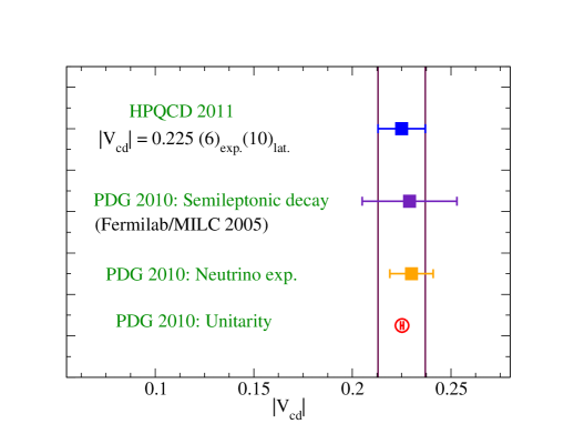
where the first error is from experiment cleo and the second is the theory error from the Lattice QCD calculation presented here. Eq.(1) is in excellent agreement with the PDG value based on neutrino scattering of |Vc​d|=0.230​(11)subscript𝑉𝑐𝑑0.23011|V_{cd}|=0.230(11).

In the rest of this article we describe how the result of eq.(1) was obtained. We work with HISQ valence charm and light quarks on the MILC AsqTad Nf=2+1subscript𝑁𝑓21N_{f}=2+1 coarse (a∼0.12similar-toπ‘Ž0.12a\sim 0.12fm) and fine (a∼0.09similar-toπ‘Ž0.09a\sim 0.09fm) lattices. Table I lists the five MILC milc1 ensembles employed in this work and some simulation parameters. Compared to dtok we have doubled the statistics on ensembles C1, C2 and F1. The valence charm and light bare quark masses are the same as in dtok with the former tuned to the Ξ·csubscriptπœ‚π‘\eta_{c} mass and the latter chosen such that the ratio of ml​i​g​h​tsubscriptπ‘šπ‘™π‘–π‘”β„Žπ‘‘m_{light} to the physical strange quark mass is approximately the same for valence and sea quarks. In the next section we summarize the formulas for hadronic matrix elements necessary to extract f+D→π​(0)subscriptsuperscriptπ‘“β†’π·πœ‹0f^{D\rightarrow\pi}_{+}(0) and explain how they are related to three- and two-point correlators evaluated numerically on the lattice. These relations are the same as those described in reference dtok so we will be brief. In section III we describe our data analysis and fitting procedures. We employ Bayesian fitting methods and carry out multi-exponential fits to several three-point and two-point correlators at the same time. Section IV discusses chiral and continuum extrapolations of lattice results to the physical limit. We apply the modified z-expansion method developed for Dβ†’K→𝐷𝐾D\rightarrow K semileptonic form factors in dtok . Section V presents our results for f+D→π​(0)subscriptsuperscriptπ‘“β†’π·πœ‹0f^{D\rightarrow\pi}_{+}(0) and |Vc​d|subscript𝑉𝑐𝑑|V_{cd}| and comparisons with other determinations of these quantities. Section VI gives a brief summary and we also include a 2n​dsuperscript2𝑛𝑑2^{nd} row unitarity test with all theory inputs coming from Lattice QCD.

Table 1: The MILC Nf=2+1subscript𝑁𝑓21N_{f}=2+1 ensembles used in the Dβ†’Ο€β†’π·πœ‹D\rightarrow\pi semileptonic project. The fourth column gives the valence HISQ light and charm quark masses in lattice units. Nc​o​n​fsubscriptπ‘π‘π‘œπ‘›π‘“N_{conf} is the number of configurations and Nt​s​r​csubscriptπ‘π‘‘π‘ π‘Ÿπ‘N_{tsrc} the number of time sources used for each configuration.
Set r1/asubscriptπ‘Ÿ1π‘Žr_{1}/a ml​(s​e​a)/ms​(s​e​a)subscriptπ‘šπ‘™π‘ π‘’π‘Žsubscriptπ‘šπ‘ π‘ π‘’π‘Žm_{l}(sea)/m_{s}(sea) a​mv​a​l​e​n​c​eπ‘Žsubscriptπ‘šπ‘£π‘Žπ‘™π‘’π‘›π‘π‘’am_{valence} Nc​o​n​fsubscriptπ‘π‘π‘œπ‘›π‘“N_{conf} Nt​s​r​csubscriptπ‘π‘‘π‘ π‘Ÿπ‘N_{tsrc} L3Γ—Ntsuperscript𝐿3subscript𝑁𝑑L^{3}\times N_{t}
C1 2.647 0.005/0.050 0.0070 1200 2 243Γ—64superscript2436424^{3}\times 64
0.6207 1200 2
C2 2.618 0.010/0.050 0.0123 1200 2 203Γ—64superscript2036420^{3}\times 64
0.6300 1200 2
C3 2.644 0.020/0.050 0.0246 600 2 203Γ—64superscript2036420^{3}\times 64
0.6235 600 2
F1 3.699 0.0062/0.031 0.00674 1200 4 283Γ—96superscript2839628^{3}\times 96
0.4130 1200 4
F2 3.712 0.0124/0.031 0.0135 600 4 283Γ—96superscript2839628^{3}\times 96
0.4120 600 4

II Relevant Matrix Elements

The most efficient way to calculate f+​(q2)subscript𝑓superscriptπ‘ž2f_{+}(q^{2}) at q2=0superscriptπ‘ž20q^{2}=0 is to focus on the scalar form factor f0​(q2)subscript𝑓0superscriptπ‘ž2f_{0}(q^{2}) and use the kinematic identity f+​(0)=f0​(0)subscript𝑓0subscript𝑓00f_{+}(0)=f_{0}(0). The scalar form factor can be determined from the matrix element of the scalar current S=Ψ¯q​Ψc𝑆subscriptΒ―Ξ¨π‘žsubscriptΨ𝑐S=\overline{\Psi}_{q}\,\Psi_{c} between the D𝐷D meson and pion states.

f0D→π​(q2)=(m0​cβˆ’m0​l)β€‹βŸ¨Ο€|S|D⟩MD2βˆ’MΟ€2.subscriptsuperscriptπ‘“β†’π·πœ‹0superscriptπ‘ž2subscriptπ‘š0𝑐subscriptπ‘š0𝑙quantum-operator-productπœ‹π‘†π·superscriptsubscript𝑀𝐷2superscriptsubscriptπ‘€πœ‹2f^{D\rightarrow\pi}_{0}(q^{2})=\frac{(m_{0c}-m_{0l})\langle\pi|S|D\rangle}{M_{D}^{2}-M_{\pi}^{2}}. (2)

The combination in the numerator of eq.(2) does not get renormalized. The use of absolutely normalized currents is one of the reasons why we are able to significantly reduce errors in our D𝐷D semileptonic scalar form factor calculations, both here and in dtok .

Our goal is to determine the hadronic matrix element βŸ¨Ο€|S|D⟩quantum-operator-productπœ‹π‘†π·\langle\pi|S|D\rangle in eq.(2) via numerical simulations. The starting point is the three-point correlator,

C3​p​n​t​(t0,t,T,pβ†’Ο€)=1L3β€‹βˆ‘xβ†’βˆ‘yβ†’βˆ‘zβ†’ei​pβ†’Ο€β‹…(zβ†’βˆ’xβ†’)superscript𝐢3𝑝𝑛𝑑subscript𝑑0𝑑𝑇subscriptβ†’π‘πœ‹1superscript𝐿3subscriptβ†’π‘₯subscript→𝑦subscript→𝑧superscript𝑒⋅𝑖subscriptβ†’π‘πœ‹β†’π‘§β†’π‘₯\displaystyle C^{3pnt}(t_{0},t,T,\vec{p}_{\pi})=\frac{1}{L^{3}}\sum_{\vec{x}}\sum_{\vec{y}}\sum_{\vec{z}}e^{i\vec{p}_{\pi}\cdot(\vec{z}-\vec{x})}
βŸ¨Ξ¦Ο€β€‹(xβ†’,t0)​S~​(zβ†’,t)​ΦD†​(yβ†’,t0βˆ’T)⟩.delimited-⟨⟩subscriptΞ¦πœ‹β†’π‘₯subscript𝑑0~𝑆→𝑧𝑑subscriptsuperscriptΦ†𝐷→𝑦subscript𝑑0𝑇\displaystyle\qquad\langle\Phi_{\pi}(\vec{x},t_{0})\,\tilde{S}(\vec{z},t)\,\Phi^{\dagger}_{D}(\vec{y},t_{0}-T)\rangle. (3)

In eq.(II) the interpolating operator Ξ¦D†subscriptsuperscriptΦ†𝐷\Phi^{\dagger}_{D} creates a D𝐷D meson at time slice t0βˆ’Tsubscript𝑑0𝑇t_{0}-T. At time t𝑑t (t0β‰₯tβ‰₯t0βˆ’Tsubscript𝑑0𝑑subscript𝑑0𝑇t_{0}\geq t\geq t_{0}-T) the scalar current S𝑆S converts the c𝑐c quark inside the D𝐷D into a light quark and also inserts momentum pβ†’Ο€subscriptβ†’π‘πœ‹\vec{p}_{\pi}. The resulting pion then propagates to time slice t0subscript𝑑0t_{0} where it is annihilated by ΦπsubscriptΞ¦πœ‹\Phi_{\pi}. In addition to the three-point correlator one needs the pion and D𝐷D meson two-point correlators,

CD2​p​n​t​(t,t0)=1L3β€‹βˆ‘xβ†’βˆ‘yβ†’βŸ¨Ξ¦D​(yβ†’,t)​ΦD†​(xβ†’,t0)⟩,subscriptsuperscript𝐢2𝑝𝑛𝑑𝐷𝑑subscript𝑑01superscript𝐿3subscriptβ†’π‘₯subscript→𝑦delimited-⟨⟩subscriptΦ𝐷→𝑦𝑑subscriptsuperscriptΦ†𝐷→π‘₯subscript𝑑0C^{2pnt}_{D}(t,t_{0})=\frac{1}{L^{3}}\sum_{\vec{x}}\sum_{\vec{y}}\langle\Phi_{D}(\vec{y},t)\Phi^{\dagger}_{D}(\vec{x},t_{0})\rangle, (4)

and

CΟ€2​p​n​t​(t,t0;pβ†’Ο€)=subscriptsuperscript𝐢2π‘π‘›π‘‘πœ‹π‘‘subscript𝑑0subscriptβ†’π‘πœ‹absent\displaystyle C^{2pnt}_{\pi}(t,t_{0};\vec{p}_{\pi})=
1L3β€‹βˆ‘xβ†’βˆ‘yβ†’ei​pβ†’Ο€β‹…(xβ†’βˆ’yβ†’)β€‹βŸ¨Ξ¦Ο€β€‹(yβ†’,t)​Φπ†​(xβ†’,t0)⟩.1superscript𝐿3subscriptβ†’π‘₯subscript→𝑦superscript𝑒⋅𝑖subscriptβ†’π‘πœ‹β†’π‘₯→𝑦delimited-⟨⟩subscriptΞ¦πœ‹β†’π‘¦π‘‘subscriptsuperscriptΞ¦β€ πœ‹β†’π‘₯subscript𝑑0\displaystyle\quad\frac{1}{L^{3}}\sum_{\vec{x}}\sum_{\vec{y}}e^{i\vec{p}_{\pi}\cdot(\vec{x}-\vec{y})}\langle\Phi_{\pi}(\vec{y},t)\Phi^{\dagger}_{\pi}(\vec{x},t_{0})\rangle. (5)

Details on how the above three- and two-point correlators can be expressed in terms of single component staggered quark propagators are given in section IV of reference dtok and will not be repeated here. There we also show how the sums βˆ‘xβ†’subscriptβ†’π‘₯\sum_{\vec{x}} in eqns.(II), (4) and (5) can be carried out using U(1) random wall sources.

The meson creation operators Ξ¦D†subscriptsuperscriptΦ†𝐷\Phi^{\dagger}_{D} and Φπ†superscriptsubscriptΞ¦πœ‹β€ \Phi_{\pi}^{\dagger} create not only the ground state D𝐷D and pion we are interested in but also an arbitrary number of excited states with the same quantum numbers. Hence the t𝑑t dependence of the two- and three-point correlators is complicated especially for staggered quarks. For two-point correlators it is given by,

CD2​p​n​t​(t)subscriptsuperscript𝐢2𝑝𝑛𝑑𝐷𝑑\displaystyle C^{2pnt}_{D}(t) =\displaystyle= βˆ‘j=0NDβˆ’1bjD​(eβˆ’EjD​t+eβˆ’EjD​(Ntβˆ’t))superscriptsubscript𝑗0subscript𝑁𝐷1subscriptsuperscript𝑏𝐷𝑗superscript𝑒subscriptsuperscript𝐸𝐷𝑗𝑑superscript𝑒subscriptsuperscript𝐸𝐷𝑗subscript𝑁𝑑𝑑\displaystyle\sum_{j=0}^{N_{D}-1}b^{D}_{j}(e^{-E^{D}_{j}t}+e^{-E^{D}_{j}(N_{t}-t)})
+\displaystyle+ βˆ‘k=0NDβ€²βˆ’1dkD​(βˆ’1)t​(eβˆ’Ek′⁣D​t+eβˆ’Ek′⁣D​(Ntβˆ’t)),superscriptsubscriptπ‘˜0superscriptsubscript𝑁𝐷′1subscriptsuperscriptπ‘‘π·π‘˜superscript1𝑑superscript𝑒subscriptsuperscriptπΈβ€²π·π‘˜π‘‘superscript𝑒superscriptsubscriptπΈπ‘˜β€²π·subscript𝑁𝑑𝑑\displaystyle\sum_{k=0}^{N_{D}^{\prime}-1}d^{D}_{k}(-1)^{t}(e^{-E^{\prime D}_{k}t}+e^{-E_{k}^{\prime D}(N_{t}-t)}),

and similarly for CΟ€2​p​n​t​(t)subscriptsuperscript𝐢2π‘π‘›π‘‘πœ‹π‘‘C^{2pnt}_{\pi}(t), except that there is no opposite parity terms for zero momentum. For three-point correlators one has

C3​p​n​t​(t,T)=βˆ‘j=0NΟ€βˆ’1βˆ‘k=0NDβˆ’1Aj​k​eβˆ’Ejπ​t​eβˆ’EkD​(Tβˆ’t)superscript𝐢3𝑝𝑛𝑑𝑑𝑇superscriptsubscript𝑗0subscriptπ‘πœ‹1superscriptsubscriptπ‘˜0subscript𝑁𝐷1subscriptπ΄π‘—π‘˜superscript𝑒superscriptsubscriptπΈπ‘—πœ‹π‘‘superscript𝑒superscriptsubscriptπΈπ‘˜π·π‘‡π‘‘\displaystyle C^{3pnt}(t,T)=\sum_{j=0}^{N_{\pi}-1}\sum_{k=0}^{N_{D}-1}A_{jk}e^{-E_{j}^{\pi}t}e^{-E_{k}^{D}(T-t)}
+βˆ‘j=0NΟ€βˆ’1βˆ‘k=0NDβ€²βˆ’1Bj​k​eβˆ’Ejπ​t​eβˆ’Ek′⁣D​(Tβˆ’t)​(βˆ’1)(Tβˆ’t)superscriptsubscript𝑗0subscriptπ‘πœ‹1superscriptsubscriptπ‘˜0superscriptsubscript𝑁𝐷′1subscriptπ΅π‘—π‘˜superscript𝑒superscriptsubscriptπΈπ‘—πœ‹π‘‘superscript𝑒superscriptsubscriptπΈπ‘˜β€²π·π‘‡π‘‘superscript1𝑇𝑑\displaystyle\quad+\sum_{j=0}^{N_{\pi}-1}\sum_{k=0}^{N_{D}^{\prime}-1}B_{jk}e^{-E_{j}^{\pi}t}e^{-E_{k}^{\prime D}(T-t)}(-1)^{(T-t)}
+βˆ‘j=0NΟ€β€²βˆ’1βˆ‘k=0NDβˆ’1Cj​k​eβˆ’Ej′⁣π​t​eβˆ’EkD​(Tβˆ’t)​(βˆ’1)tsuperscriptsubscript𝑗0superscriptsubscriptπ‘πœ‹β€²1superscriptsubscriptπ‘˜0subscript𝑁𝐷1subscriptπΆπ‘—π‘˜superscript𝑒superscriptsubscriptπΈπ‘—β€²πœ‹π‘‘superscript𝑒superscriptsubscriptπΈπ‘˜π·π‘‡π‘‘superscript1𝑑\displaystyle\quad+\sum_{j=0}^{N_{\pi}^{\prime}-1}\sum_{k=0}^{N_{D}-1}C_{jk}e^{-E_{j}^{\prime\pi}t}e^{-E_{k}^{D}(T-t)}(-1)^{t}
+βˆ‘j=0NΟ€β€²βˆ’1βˆ‘k=0NDβ€²βˆ’1Dj​k​eβˆ’Ej′⁣π​t​eβˆ’Ek′⁣D​(Tβˆ’t)​(βˆ’1)t​(βˆ’1)(Tβˆ’t).superscriptsubscript𝑗0superscriptsubscriptπ‘πœ‹β€²1superscriptsubscriptπ‘˜0superscriptsubscript𝑁𝐷′1subscriptπ·π‘—π‘˜superscript𝑒superscriptsubscriptπΈπ‘—β€²πœ‹π‘‘superscript𝑒superscriptsubscriptπΈπ‘˜β€²π·π‘‡π‘‘superscript1𝑑superscript1𝑇𝑑\displaystyle\quad+\sum_{j=0}^{N_{\pi}^{\prime}-1}\sum_{k=0}^{N_{D}^{\prime}-1}D_{jk}e^{-E_{j}^{\prime\pi}t}e^{-E_{k}^{\prime D}(T-t)}(-1)^{t}(-1)^{(T-t)}.

We are interested in the ground state contributions with amplitudes,

b0D≑|⟨ΦD|D⟩|22​MD​a3,subscriptsuperscript𝑏𝐷0superscriptinner-productsubscriptΦ𝐷𝐷22subscript𝑀𝐷superscriptπ‘Ž3b^{D}_{0}\equiv\frac{|\langle\Phi_{D}|D\rangle|^{2}}{2M_{D}a^{3}}, (8)
b0π≑|βŸ¨Ξ¦Ο€|Ο€βŸ©|22​Eπ​a3,subscriptsuperscriptπ‘πœ‹0superscriptinner-productsubscriptΞ¦πœ‹πœ‹22subscriptπΈπœ‹superscriptπ‘Ž3b^{\pi}_{0}\equiv\frac{|\langle\Phi_{\pi}|\pi\rangle|^{2}}{2E_{\pi}a^{3}}, (9)

and

A00β‰‘βŸ¨Ξ¦Ο€|Ο€βŸ©β€‹βŸ¨Ο€|S|DβŸ©β€‹βŸ¨D|Ξ¦D⟩(2​Eπ​a3)​(2​MD​a3)​a3.subscript𝐴00inner-productsubscriptΞ¦πœ‹πœ‹quantum-operator-productπœ‹π‘†π·inner-product𝐷subscriptΦ𝐷2subscriptπΈπœ‹superscriptπ‘Ž32subscript𝑀𝐷superscriptπ‘Ž3superscriptπ‘Ž3A_{00}\equiv\frac{\langle\Phi_{\pi}|\pi\rangle\,\langle\pi|S|D\rangle\,\langle D|\Phi_{D}\rangle}{(2E_{\pi}a^{3})\,(2M_{D}a^{3})}\,a^{3}. (10)

So the hadronic matrix element βŸ¨Ο€|S|D⟩quantum-operator-productπœ‹π‘†π·\langle\pi|S|D\rangle that enters into the formula for f0D→π​(0)subscriptsuperscriptπ‘“β†’π·πœ‹00f^{D\rightarrow\pi}_{0}(0) in (2) is given by,

βŸ¨Ο€|S|D⟩=2​MD​Eπ​A00b0π​b0D.quantum-operator-productπœ‹π‘†π·2subscript𝑀𝐷subscriptπΈπœ‹subscript𝐴00superscriptsubscript𝑏0πœ‹superscriptsubscript𝑏0𝐷\langle\pi|S|D\rangle=2\sqrt{M_{D}E_{\pi}}\;\frac{A_{00}}{\sqrt{b_{0}^{\pi}b_{0}^{D}}}. (11)

We have accumulated simulation data for zero momentum D𝐷D correlators and for pion correlators with momenta 2​πL​(0,0,0)2πœ‹πΏ000\frac{2\pi}{L}(0,0,0), 2​πL​(1,0,0)2πœ‹πΏ100\frac{2\pi}{L}(1,0,0), 2​πL​(1,1,0)2πœ‹πΏ110\frac{2\pi}{L}(1,1,0) and 2​πL​(1,1,1)2πœ‹πΏ111\frac{2\pi}{L}(1,1,1). The corresponding three-point correlators were calculated for T=15,16𝑇1516T=15,16 on the coarse and for T=19,20,23𝑇192023T=19,20,23 on the fine ensembles. In the next section we describe how the combination on the right-hand-side of (11) is obtained from three- and two-point correlators.

III Fits and Data Analysis
Refer to caption
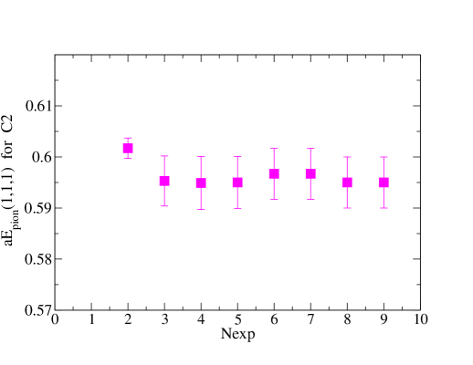
Figure 1: Ground state pion energy in lattice units for momentum 2​πL​(1,1,1)2πœ‹πΏ111\frac{2\pi}{L}(1,1,1) versus the number of exponentials in the fit.
Refer to caption
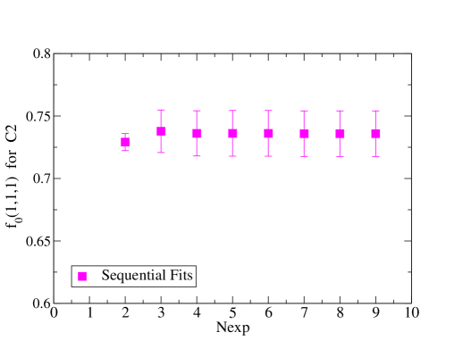
Figure 2: The form factor f0​(q2)subscript𝑓0superscriptπ‘ž2f_{0}(q^{2}) for pion momentum 2​πL​(1,1,1)2πœ‹πΏ111\frac{2\pi}{L}(1,1,1) from simultaneous fits to two- and three-point correlators versus Ne​x​p=ND=NDβ€²=NΟ€=NΟ€β€²subscript𝑁𝑒π‘₯𝑝subscript𝑁𝐷subscriptsuperscript𝑁′𝐷subscriptπ‘πœ‹subscriptsuperscriptπ‘β€²πœ‹N_{exp}=N_{D}=N^{\prime}_{D}=N_{\pi}=N^{\prime}_{\pi}. The β€œsequential fitting” method was employed to go from one Ne​x​psubscript𝑁𝑒π‘₯𝑝N_{exp} value to the next. In this method the fit results from the Ne​x​psubscript𝑁𝑒π‘₯𝑝N_{exp} exponential fit is inserted as initial conditions for the subsequent [Ne​x​psubscript𝑁𝑒π‘₯𝑝N_{exp} + 1] exponential fit.

Extracting energies and amplitudes from numerical data on two- and three-point correlators is one of the more challenging but at the same time very important aspect of lattice calculations. For the past decade the HPQCD collaboration has been employing fitting methods based on Bayesian statistics and involving multi-exponential fits bayse . For instance, in order to obtain the ground state energy and amplitude from a two-point correlator, we drop the first 1 ∼similar-to\sim 4 time slices and then fit to the form of eq.(II) for several values of N≑ND𝑁subscript𝑁𝐷N\equiv N_{D} (or NΟ€subscriptπ‘πœ‹N_{\pi}) and Nβ€²superscript𝑁′N^{\prime}. One continues to increase the number of exponentials until the fit results for E0subscript𝐸0E_{0} and b0subscript𝑏0b_{0} including their errors and the chisquared per degree of freedom of the fit have stabilized. Fig.1 shows an example of a​EΟ€π‘ŽsubscriptπΈπœ‹aE_{\pi} versus Ne​x​p=NΟ€subscript𝑁𝑒π‘₯𝑝subscriptπ‘πœ‹N_{exp}=N_{\pi} for momentum 2​πL​(1,1,1)2πœ‹πΏ111\frac{2\pi}{L}(1,1,1) with NΟ€β€²=NΟ€subscriptsuperscriptπ‘β€²πœ‹subscriptπ‘πœ‹N^{\prime}_{\pi}=N_{\pi}. One sees that fits have stabilized after Ne​x​p=3subscript𝑁𝑒π‘₯𝑝3N_{exp}=3. It should be noted that as one increases the number of exponentials and with it the number of fit parameters, the number of data points is growing as well. Each new fit parameter adds another prior term, i.e. additional data, to the fit function and the number of data points minus the number of fit parameters remains constant bayse .

The combination A00b0π​b0Dsubscript𝐴00superscriptsubscript𝑏0πœ‹superscriptsubscript𝑏0𝐷\frac{A_{00}}{\sqrt{b_{0}^{\pi}b_{0}^{D}}} is obtained from simultaneous fits to CD2​p​n​t​(t)subscriptsuperscript𝐢2𝑝𝑛𝑑𝐷𝑑C^{2pnt}_{D}(t), CΟ€2​p​n​t​(t)subscriptsuperscript𝐢2π‘π‘›π‘‘πœ‹π‘‘C^{2pnt}_{\pi}(t) and C3​p​n​t​(t,T)superscript𝐢3𝑝𝑛𝑑𝑑𝑇C^{3pnt}(t,T) for 2 (or 3) T𝑇T values. In order to be able to include a large number of exponentials in these complicated fits we proceed as follows. We set NΟ€=NΟ€β€²=ND=ND′≑Ne​x​psubscriptπ‘πœ‹subscriptsuperscriptπ‘β€²πœ‹subscript𝑁𝐷subscriptsuperscript𝑁′𝐷subscript𝑁𝑒π‘₯𝑝N_{\pi}=N^{\prime}_{\pi}=N_{D}=N^{\prime}_{D}\equiv N_{exp} and start out with a small value, Ne​x​p=2subscript𝑁𝑒π‘₯𝑝2N_{exp}=2 or Ne​x​p=3subscript𝑁𝑒π‘₯𝑝3N_{exp}=3. The fit results are then inserted as initial conditions for the subsequent Ne​x​p+1subscript𝑁𝑒π‘₯𝑝1N_{exp}+1 exponential fit. This procedure is repeated until one has completed multi-exponential fits with Ne​x​psubscript𝑁𝑒π‘₯𝑝N_{exp} much larger than 2. Fig. 2 shows results for f0​(q2)subscript𝑓0superscriptπ‘ž2f_{0}(q^{2}) on ensemble C2 at pion momentum 2​πL​(1,1,1)2πœ‹πΏ111\frac{2\pi}{L}(1,1,1) versus Ne​x​psubscript𝑁𝑒π‘₯𝑝N_{exp} using this β€œsequential fitting” procedure. One sees that, similar to in Fig.1, fit results have stabilized for Ne​x​p>3subscript𝑁𝑒π‘₯𝑝3N_{exp}>3 fnote1 .

In ongoing work we are investigating further methods to deal with complicated fits with large number of parameters, in particular fits to collections of sums of exponentials marginal . For the calculations of this article, however, we have found that the β€œsequential fitting” method described above works well for all our data fnote2 . We are even able to fit data on a given ensemble for all four pion momenta simultaneously and this allows us to obtain correlations between form factor results at different q2superscriptπ‘ž2q^{2}. These simultaneous fit results for f0​(pβ†’Ο€)subscript𝑓0subscriptβ†’π‘πœ‹f_{0}(\vec{p}_{\pi}) are given in Table II for several pion momenta pβ†’Ο€subscriptβ†’π‘πœ‹\vec{p}_{\pi} (the latter in units of 2​πL)\frac{2\pi}{L}).

IV Chiral and Continuum Extrapolation

The next step is to extrapolate the data of Table II to the chiral/continuum limit. We do so using the β€œmodified z-expansion fit” developed in dtok . The scalar form factor is parameterized as

f0​(q2)subscript𝑓0superscriptπ‘ž2\displaystyle f_{0}(q^{2}) =\displaystyle= 1P​(q2)​Φ0​(a0​D0+a1​D1​z+a2​D2​z2)1𝑃superscriptπ‘ž2subscriptΞ¦0subscriptπ‘Ž0subscript𝐷0subscriptπ‘Ž1subscript𝐷1𝑧subscriptπ‘Ž2subscript𝐷2superscript𝑧2\displaystyle\frac{1}{P(q^{2})\Phi_{0}}\left(a_{0}D_{0}+a_{1}D_{1}z+a_{2}D_{2}z^{2}\right) (12)
Γ—(1+b1​(a​EΟ€)2+b2​(a​EΟ€)4),absent1subscript𝑏1superscriptπ‘ŽsubscriptπΈπœ‹2subscript𝑏2superscriptπ‘ŽsubscriptπΈπœ‹4\displaystyle\times\left(1+b_{1}(aE_{\pi})^{2}+b_{2}(aE_{\pi})^{4}\right),

with

Disubscript𝐷𝑖\displaystyle D_{i} =\displaystyle= 1+c1i​xl+c2i​xl​l​o​g​(xl)+di​(a​mc)2+ei​(a​mc)41superscriptsubscript𝑐1𝑖subscriptπ‘₯𝑙superscriptsubscript𝑐2𝑖subscriptπ‘₯π‘™π‘™π‘œπ‘”subscriptπ‘₯𝑙subscript𝑑𝑖superscriptπ‘Žsubscriptπ‘šπ‘2subscript𝑒𝑖superscriptπ‘Žsubscriptπ‘šπ‘4\displaystyle 1+c_{1}^{i}x_{l}+c_{2}^{i}x_{l}log(x_{l})+d_{i}(am_{c})^{2}+e_{i}(am_{c})^{4} (13)
+fi​(12​δ​MΟ€2+δ​MK2),subscript𝑓𝑖12𝛿superscriptsubscriptπ‘€πœ‹2𝛿superscriptsubscript𝑀𝐾2\displaystyle+f_{i}\left(\frac{1}{2}\delta M_{\pi}^{2}+\delta M_{K}^{2}\right),
xl=MΟ€2(4​π​fΟ€)2,subscriptπ‘₯𝑙superscriptsubscriptπ‘€πœ‹2superscript4πœ‹subscriptπ‘“πœ‹2x_{l}=\frac{M_{\pi}^{2}}{(4\pi f_{\pi})^{2}}, (14)
δ​MΟ€2=1(4​π​fΟ€)2​((MΟ€s​e​a)2βˆ’(MΟ€v​a​l​e​n​c​e)2),𝛿superscriptsubscriptπ‘€πœ‹21superscript4πœ‹subscriptπ‘“πœ‹2superscriptsuperscriptsubscriptπ‘€πœ‹π‘ π‘’π‘Ž2superscriptsuperscriptsubscriptπ‘€πœ‹π‘£π‘Žπ‘™π‘’π‘›π‘π‘’2\delta M_{\pi}^{2}=\frac{1}{(4\pi f_{\pi})^{2}}\left((M_{\pi}^{sea})^{2}-(M_{\pi}^{valence})^{2}\right), (15)
δ​MK2=1(4​π​fΟ€)2​((MKs​e​a)2βˆ’(MKv​a​l​e​n​c​e)2).𝛿superscriptsubscript𝑀𝐾21superscript4πœ‹subscriptπ‘“πœ‹2superscriptsuperscriptsubscriptπ‘€πΎπ‘ π‘’π‘Ž2superscriptsuperscriptsubscriptπ‘€πΎπ‘£π‘Žπ‘™π‘’π‘›π‘π‘’2\delta M_{K}^{2}=\frac{1}{(4\pi f_{\pi})^{2}}\left((M_{K}^{sea})^{2}-(M_{K}^{valence})^{2}\right). (16)

The kinematic variable z𝑧z is defined as bgl ; arnesen ; bhill ,

z​(q2,t0)=t+βˆ’q2βˆ’t+βˆ’t0t+βˆ’q2+t+βˆ’t0,𝑧superscriptπ‘ž2subscript𝑑0subscript𝑑superscriptπ‘ž2subscript𝑑subscript𝑑0subscript𝑑superscriptπ‘ž2subscript𝑑subscript𝑑0z(q^{2},t_{0})=\frac{\sqrt{t_{+}-q^{2}}-\sqrt{t_{+}-t_{0}}}{\sqrt{t_{+}-q^{2}}+\sqrt{t_{+}-t_{0}}}, (17)

with t0subscript𝑑0t_{0} a free parameter (which we set equal to 1.951.951.95GeV2 ) and tΒ±=(MDΒ±MΟ€)2subscript𝑑plus-or-minussuperscriptplus-or-minussubscript𝑀𝐷subscriptπ‘€πœ‹2t_{\pm}=(M_{D}\pm M_{\pi})^{2}. We take Ξ¦0subscriptΞ¦0\Phi_{0} from arnesen and set P​(q2)=1𝑃superscriptπ‘ž21P(q^{2})=1, where the latter relation reflects the absence of subthreshold poles in the scalar channel.

Table 2: Results for f0​(pβ†’Ο€)subscript𝑓0subscriptβ†’π‘πœ‹f_{0}(\vec{p}_{\pi}) for each ensemble
Set f0​(0,0,0)subscript𝑓0000f_{0}(0,0,0) f0​(1,0,0)subscript𝑓0100f_{0}(1,0,0) f0​(1,1,0)subscript𝑓0110f_{0}(1,1,0) f0​(1,1,1)subscript𝑓0111f_{0}(1,1,1)
C1 1.1557(74) 0.9155(93) 0.8119(68) 0.7384(209)
C2 1.1014(38) 0.8700(59) 0.7801(43) 0.7315(87)
C3 1.0398(28) 0.8787(36) 0.7922(31) 0.7326(66)
F1 1.1053(29) 0.8652(52) 0.7586(53) 0.7112(108)
F2 1.0443(28) 0.8613(31) 0.7645(53) 0.7097(70)
Refer to caption
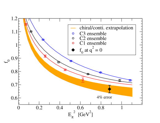
Figure 3: Chiral/continuum extrapolation of f0Dβ†’Ο€subscriptsuperscriptπ‘“β†’π·πœ‹0f^{D\rightarrow\pi}_{0} versus EΟ€2superscriptsubscriptπΈπœ‹2E_{\pi}^{2}. The data points are from the coarse ensembles (C1, C2 and C3). The three individual curves and the extrapolated band are from a fit to all five ensembles.
Refer to caption
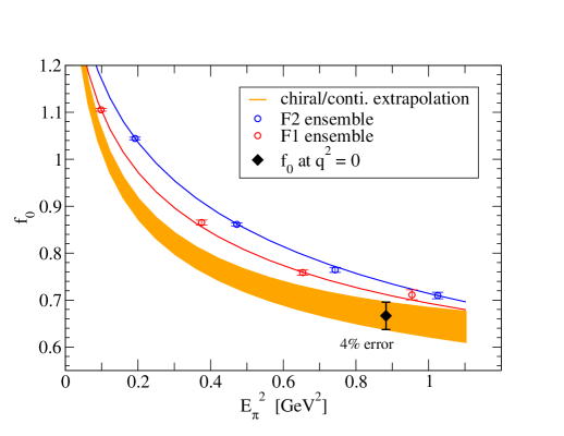
Figure 4: Same as for Fig.3 showing, however, the fine data points.
Refer to caption
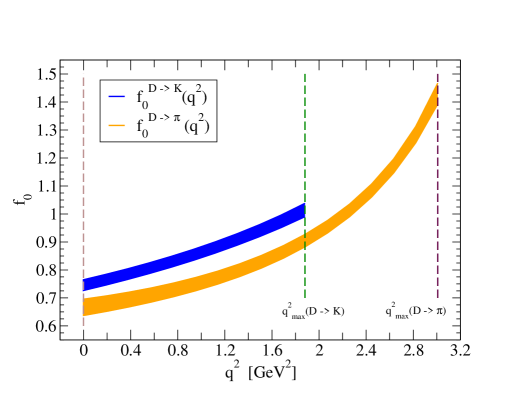
Figure 5: f0Dβ†’K​(q2)superscriptsubscript𝑓0→𝐷𝐾superscriptπ‘ž2f_{0}^{D\rightarrow K}(q^{2}) and f0D→π​(q2)superscriptsubscript𝑓0β†’π·πœ‹superscriptπ‘ž2f_{0}^{D\rightarrow\pi}(q^{2}) versus q2superscriptπ‘ž2q^{2} in the physical limit.

We show results of fits to the form of eq.(12) in Figs.3 & 4. We plot separately the coarse and fine data points in order to be able to better distinguish individual curves. However, the fit was done simultaneously to all the data in Table II, coarse and fine. The Ο‡2/d​o​f=0.85superscriptπœ’2π‘‘π‘œπ‘“0.85\chi^{2}/dof=0.85 for this fit. In Fig.5 we show both f0Dβ†’K​(q2)superscriptsubscript𝑓0→𝐷𝐾superscriptπ‘ž2f_{0}^{D\rightarrow K}(q^{2}) (results from dtok ) and f0D→π​(q2)superscriptsubscript𝑓0β†’π·πœ‹superscriptπ‘ž2f_{0}^{D\rightarrow\pi}(q^{2}) versus q2superscriptπ‘ž2q^{2} in the physical region 0≀q2≀qm​a​x2=(MDβˆ’Mπ​(K))20superscriptπ‘ž2subscriptsuperscriptπ‘ž2π‘šπ‘Žπ‘₯superscriptsubscript𝑀𝐷subscriptπ‘€πœ‹πΎ20\leq q^{2}\leq q^{2}_{max}=(M_{D}-M_{\pi(K)})^{2}. Note that we consider the correlations between the momenta in the fits which we did not consider in dtok . However, we find that including or excluding correlations in our chiral/continuum extrapolations has minimal effect on f0D→π​(0)superscriptsubscript𝑓0β†’π·πœ‹0f_{0}^{D\rightarrow\pi}(0) at the physical point, namely a ∼0.04​σsimilar-toabsent0.04𝜎\sim 0.04\sigma shift in the central value and a ∼0.02​σsimilar-toabsent0.02𝜎\sim 0.02\sigma change in the error.

The motivation for the β€œmodified z-expansion fit” is explained in more detail in dtok . Form factors at q2=0superscriptπ‘ž20q^{2}=0 are needed to extract the CKM matrix elements |Vc​d|subscript𝑉𝑐𝑑|V_{cd}| or |Vc​s|subscript𝑉𝑐𝑠|V_{cs}|. The pion energy approaches 1GeV in this kinematic region and so chiral perturbation theory might cease to be valid. The z-expansion, on the other hand, is applicable throughout the physical kinematic region, and our new β€œmodified z-expansion” allows for the expansion coefficients to be mass and lattice spacing dependent. We have checked that fits to eq.(12) are stable with respect to adding further terms such as xl2superscriptsubscriptπ‘₯𝑙2x_{l}^{2}, (a​mc)6superscriptπ‘Žsubscriptπ‘šπ‘6(am_{c})^{6}, (a​EΟ€)6superscriptπ‘ŽsubscriptπΈπœ‹6(aE_{\pi})^{6} or keeping just the c1isubscriptsuperscript𝑐𝑖1c^{i}_{1} and c2isubscriptsuperscript𝑐𝑖2c^{i}_{2} terms in eq.(13) (the Disubscript𝐷𝑖D_{i}’s). Such changes in the fit ansatz led to minimal changes in both the central value and the error for f0​(0)subscript𝑓00f_{0}(0) in the physical limit. We have also verified that traditional ChPT extrapolations (see Appendix C & D of dtok and references therein for relevant ChPT formulas) lead to f+​(0)subscript𝑓0f_{+}(0) in the physical limit consistent with the z-expansion result and with comparable errors, however with worse Ο‡2/d​o​fsuperscriptπœ’2π‘‘π‘œπ‘“\chi^{2}/dof.

V Results for f+D→π​(0)subscriptsuperscriptπ‘“β†’π·πœ‹0f^{D\rightarrow\pi}_{+}(0) and |Vc​d|subscript𝑉𝑐𝑑|V_{cd}| in the Physical Limit

Table 3: Error Budget for f+D→π​(0)subscriptsuperscriptπ‘“β†’π·πœ‹0f^{D\rightarrow\pi}_{+}(0)
Type Error (%)
Statistical 3.1
Scale (r1subscriptπ‘Ÿ1r_{1} and r1/asubscriptπ‘Ÿ1π‘Žr_{1}/a) 0.7
Expansion coeff. aisubscriptπ‘Žπ‘–a_{i} 0.3
Epsubscript𝐸𝑝E_{p} 0.6
Light quark dependence 1.9
Sea quark dependence 0.6
a​mcπ‘Žsubscriptπ‘šπ‘am_{c} corrections 2.0
a​EΟ€π‘ŽsubscriptπΈπœ‹aE_{\pi} corrections 1.0
Finite volume 0.04
Charm mass tuning 0.05
Total 4.4%

Our final result for the Dβ†’Ο€β†’π·πœ‹D\rightarrow\pi form factor at q2=0superscriptπ‘ž20q^{2}=0 averaged over D0β†’Ο€βˆ’β†’superscript𝐷0superscriptπœ‹D^{0}\rightarrow\pi^{-} and D+β†’Ο€0β†’superscript𝐷superscriptπœ‹0D^{+}\rightarrow\pi^{0}, is,

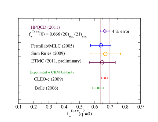
f+D→π​(0)=0.666​(20)s​t​a​t.​(21)s​y​s.,superscriptsubscriptπ‘“β†’π·πœ‹00.666subscript20π‘ π‘‘π‘Žπ‘‘subscript21𝑠𝑦𝑠f_{+}^{D\rightarrow\pi}(0)=0.666(20)_{stat.}(21)_{sys.}, (18)

where the first error is statistical and the second systematic. Fig.6 plots our new result together with other theory calculations fermi2005 ; sumrule ; etmcf0 and experimental determinations cleo ; belle (the latter use CKM unitarity values for |Vc​d|subscript𝑉𝑐𝑑|V_{cd}| to extract f+D→π​(0)subscriptsuperscriptπ‘“β†’π·πœ‹0f^{D\rightarrow\pi}_{+}(0)).

The total error in our f+D→π​(0)subscriptsuperscriptπ‘“β†’π·πœ‹0f^{D\rightarrow\pi}_{+}(0) is 4.44.44.4%, signifying a better than factor of 2 improvement over previous lattice determinations. The full error budget is given in Table III. The largest error is statistical followed by a​mcπ‘Žsubscriptπ‘šπ‘am_{c} and light quark mass dependence errors. All but the last two entries in Table III were obtained using the methods described in reference alpha and Appendix B of dtok . For instance, the β€œlight quark dependence” errors come from the c1isuperscriptsubscript𝑐1𝑖c_{1}^{i} and c2isuperscriptsubscript𝑐2𝑖c_{2}^{i} terms in the fit ansatz eq.(13), the β€œa​mcπ‘Žsubscriptπ‘šπ‘am_{c} corrections” from the disubscript𝑑𝑖d_{i} and eisubscript𝑒𝑖e_{i} terms etc.

Finite volume errors were estimated by calculating a pion tadpole integral both at finite and at infinite volume. The charm mass tuning error is taken to be the same as for Dβ†’K,lβ€‹Ξ½β†’π·πΎπ‘™πœˆD\rightarrow K,l\nu for which calculations at two values of a​mcπ‘Žsubscriptπ‘šπ‘am_{c} were carried out explicitely to estimate this error. Effects from electromagnetism/isospin breaking and charm sea are expected to give negligible contribution to the error budget compared to our other errors (see dtok ).

Finally one can combine our result for f+D→π​(0)subscriptsuperscriptπ‘“β†’π·πœ‹0f^{D\rightarrow\pi}_{+}(0) with CLEO-c’s measurement of |Vc​d|Γ—f+D→π​(0)subscript𝑉𝑐𝑑subscriptsuperscriptπ‘“β†’π·πœ‹0|V_{cd}|\times f^{D\rightarrow\pi}_{+}(0) cleo to extract a precision value for |Vc​d|subscript𝑉𝑐𝑑|V_{cd}| from D semileptonic decays. This leads to the result quoted already in eq.(1), which is shown in Fig.7 together with values from PDG2010.

VI Summary

Refer to caption
Figure 6: The Dβ†’Ο€β†’π·πœ‹D\rightarrow\pi form factor f+D→π​(0)subscriptsuperscriptπ‘“β†’π·πœ‹0f^{D\rightarrow\pi}_{+}(0) from this work and comparisons with other determinations fermi2005 ; sumrule ; etmcf0 ; cleo ; belle .
Refer to caption
Figure 7: Comparison of |Vc​d|subscript𝑉𝑐𝑑|V_{cd}| from this work with values in PDG2010 pdg2010 .

In this article we have presented a new calculation of the Dβ†’Ο€,lβ€‹Ξ½β†’π·πœ‹π‘™πœˆD\rightarrow\pi,l\nu semileptonic form factor f+D→π​(q2)subscriptsuperscriptπ‘“β†’π·πœ‹superscriptπ‘ž2f^{D\rightarrow\pi}_{+}(q^{2}) at q2=0superscriptπ‘ž20q^{2}=0, with errors a factor of two better than in the past. This combined with recent precision measurement of the branching fraction for this process by CLEO-c has allowed for an accurate determination of the CKM matrix element |Vc​d|subscript𝑉𝑐𝑑|V_{cd}|. Direct determination of |Vc​d|subscript𝑉𝑐𝑑|V_{cd}| from D𝐷D semileptonic decays is becoming competitive with that from neutrino scattering. The fact that these two very different processes lead to the same |Vc​d|subscript𝑉𝑐𝑑|V_{cd}| is a nontrivial consistency check of the Standard Model.

Finally using our values for |Vc​d|subscript𝑉𝑐𝑑|V_{cd}| and |Vc​s|subscript𝑉𝑐𝑠|V_{cs}| dtok plus the most recent |Vc​b|e​x​c​l.=0.0397​(10)subscriptsubscript𝑉𝑐𝑏𝑒π‘₯𝑐𝑙0.039710|V_{cb}|_{excl.}=0.0397(10) from the Fermilab Lattice & MILC collaborations vcb , the most up-to-date test of second row unitary from Lattice QCD becomes,

|Vc​d|2+|Vc​s|2+|Vc​b|2=0.976​(50).superscriptsubscript𝑉𝑐𝑑2superscriptsubscript𝑉𝑐𝑠2superscriptsubscript𝑉𝑐𝑏20.97650|V_{cd}|^{2}+|V_{cs}|^{2}+|V_{cb}|^{2}=0.976(50). (19)

This improves on the PDG2010 value 1.101​(74)1.101741.101(74) pdg2010 .

In the future we will be reducing the largest errors in Table III by increasing statistics and simulating on finer lattices jona . Calculations of the full q2superscriptπ‘ž2q^{2} dependence of f+Dβ†’K​(q2)superscriptsubscript𝑓→𝐷𝐾superscriptπ‘ž2f_{+}^{D\rightarrow K}(q^{2}) and f+D→π​(q2)superscriptsubscriptπ‘“β†’π·πœ‹superscriptπ‘ž2f_{+}^{D\rightarrow\pi}(q^{2}) are also already underway jona . Furthermore we are working on updating HPQCD’s result for the D𝐷D meson decay constant fDsubscript𝑓𝐷f_{D} follana and on carrying out an independent extraction of |Vc​d|subscript𝑉𝑐𝑑|V_{cd}| from D𝐷D leptonic decays pacs .

Acknowledgments:
This work was supported by the DOE and NSF in the US, by STFC in the UK and by MICINN and DGIID-DGA in Spain. We thank MILC for making their Lattices available. Simulations were carried out on facilities of the USQCD collaboration funded by the Office of Science of the DOE and at the Ohio Supercomputer Center.

Appendix A Priors and Prior Widths for Two- and Three-Point Correlators

In this appendix we give sample priors and prior widths used in the fits of section III (the reader is referred to reference bayse for definitions of these terms). We turn to the Particle Data Group listings for guidance in picking priors for energies and energy splittings. All energies in Table IV are given in lattices units and are appropriate for ensemble C2. Numbers for other ensembles can be obtained by rescaling with corresponding lattice spacings. Prior widths for amplitudes are fixed based on exploratory initial fits.

Table 4: Sample priors and prior widths for two- and three-point correlator fits. Energies are in lattice units, and this example corresponds to priors used for ensemble C2. The notation is the same as in equations (II) and (II).
prior prior width
E0Dsubscriptsuperscript𝐸𝐷0E^{D}_{0} 1.16 0.58
Ej>0Dβˆ’Ejβˆ’1Dsubscriptsuperscript𝐸𝐷𝑗0subscriptsuperscript𝐸𝐷𝑗1E^{D}_{j>0}-E^{D}_{j-1} 0.36 0.36
E0′⁣Dsubscriptsuperscript𝐸′𝐷0E^{\prime D}_{0} 1.52 1.52
Ek>0′⁣Dβˆ’Ekβˆ’1′⁣DsubscriptsuperscriptπΈβ€²π·π‘˜0subscriptsuperscriptπΈβ€²π·π‘˜1E^{\prime D}_{k>0}-E^{\prime D}_{k-1} 0.36 0.36
bjDsubscriptsuperscript𝑏𝐷𝑗\sqrt{b^{D}_{j}} 0.01 0.5
dkDsubscriptsuperscriptπ‘‘π·π‘˜\sqrt{d^{D}_{k}} 0.01 0.5
E0π​(000)subscriptsuperscriptπΈπœ‹0000E^{\pi}_{0}(000) 0.21 0.11
E0π​(100)subscriptsuperscriptπΈπœ‹0100E^{\pi}_{0}(100) 0.38 0.19
E0π​(110)subscriptsuperscriptπΈπœ‹0110E^{\pi}_{0}(110) 0.49 0.25
E0π​(111)subscriptsuperscriptπΈπœ‹0111E^{\pi}_{0}(111) 0.60 0.30
E1π​(a​l​l​m​o​m)βˆ’E0π​(a​l​l​m​o​m)subscriptsuperscriptπΈπœ‹1π‘Žπ‘™π‘™π‘šπ‘œπ‘šsubscriptsuperscriptπΈπœ‹0π‘Žπ‘™π‘™π‘šπ‘œπ‘šE^{\pi}_{1}(all\;\;mom)-E^{\pi}_{0}(all\;\;mom) 0.61 0.31
Ej>1π​(a​l​l​m​o​m)βˆ’Ejβˆ’1π​(a​l​l​m​o​m)subscriptsuperscriptπΈπœ‹π‘—1π‘Žπ‘™π‘™π‘šπ‘œπ‘šsubscriptsuperscriptπΈπœ‹π‘—1π‘Žπ‘™π‘™π‘šπ‘œπ‘šE^{\pi}_{j>1}(all\;\;mom)-E^{\pi}_{j-1}(all\;\;mom) 0.36 0.36
E0′⁣π​(100)subscriptsuperscriptπΈβ€²πœ‹0100E^{\prime\pi}_{0}(100) 0.74 0.74
E0′⁣π​(110)subscriptsuperscriptπΈβ€²πœ‹0110E^{\prime\pi}_{0}(110) 0.85 0.85
E0′⁣π​(111)subscriptsuperscriptπΈβ€²πœ‹0111E^{\prime\pi}_{0}(111) 0.96 0.96
Ek>0′⁣π​(m​o​m>0)βˆ’Ekβˆ’1′⁣π​(m​o​m>0)subscriptsuperscriptπΈβ€²πœ‹π‘˜0π‘šπ‘œπ‘š0subscriptsuperscriptπΈβ€²πœ‹π‘˜1π‘šπ‘œπ‘š0E^{\prime\pi}_{k>0}(mom>0)-E^{\prime\pi}_{k-1}(mom>0) 0.36 0.36
bjπ​(a​l​l​m​o​m)subscriptsuperscriptπ‘πœ‹π‘—π‘Žπ‘™π‘™π‘šπ‘œπ‘š\sqrt{b^{\pi}_{j}}(all\;\;mom) 0.01 0.5
dkπ​(m​o​m>0)subscriptsuperscriptπ‘‘πœ‹π‘˜π‘šπ‘œπ‘š0\sqrt{d^{\pi}_{k}}(mom>0) 0.01 0.5
Aj​ksubscriptπ΄π‘—π‘˜A_{jk}, Bj​ksubscriptπ΅π‘—π‘˜B_{jk}, Cj​ksubscriptπΆπ‘—π‘˜C_{jk}, Dj​ksubscriptπ·π‘—π‘˜D_{jk} 0.01 0.1

References

  • (1) For some recent reviews see :
    R.Β Van de Water, PoS LAT2009, 014 (2009;
    V.Β Lubicz, PoS LAT2009, 013 (2009);
    J.Β Laiho, E.Β Lunghi and R.Β Van de Water, Phys.Β Rev.Β  D81, 034503 (2010);
    J.Β Shigemitsu, [arXiv:1102.0716 [hep-ph]];
    J.Β Laiho, B.D.Β Pecjak and C.Β Schwanda, [arXiv:1107.3934 [hep-ex]].
  • (2) P.Β A.Β Boyle et al. [UKQCD/RBC collaboration]; Eur.Β Phys.Β J.Β  C69, 159-167 (2010).
  • (3) V.Β Lubicz et al., [ETMC], Phys.Β Rev.Β  D 80, 111502 (2009)
  • (4) A.Β Bazavov et al. [MILC], PoS LATTICE2010, 074 (2010).
  • (5) E.Β Follana et al., [HPQCD/UKQCD Collaboration], Phys.Β Rev.Β Lett.Β  100, 062002 (2008)
  • (6) S.Β Durr et al., [BMW Collaboration], Phys.Β Rev.Β  D 81, 054507 (2010)
  • (7) Y.Β Aoki et al. [RBC/UKQCD Collaboration], [arXiv:1011.0892 [hep-lat]].
  • (8) B.Β Blossier et al. [ETMC], JHEP 0907, 043 (2009)
  • (9) M.Β Antonelli et al., [FlaviaNet Working Group on Kaon Decays], Eur.Β Phys.Β J.Β  C 69, 399 (2010)
  • (10) H.Β Na et al., [HPQCD collaboration], Phys.Β Rev.Β  D 82, 114506 (2010)
  • (11) E.Β Follana et al. [HPQCD/UKQCD Collaboration], Phys.Β Rev.Β  D75, 054502 (2007).
  • (12) D.Β Besson et al. [CLEO Collaboration], Phys.Β Rev.Β  D 80, 032005 (2009)
  • (13) C.Aubin et al., [Fermilab Lattice & MILC collaborations]; Phys. Rev. Lett. 94, 011601 (2005).
  • (14) K.Β Nakamura et al. [Particle Data Group], J.Β Phys.Β G 37, 075021 (2010).
  • (15) C.Β Bernard et al. [MILC]; Phys.Β Rev.Β  D64, 054506 (2001).
  • (16) G.P.Β Lepage et al. [HPQCD collaboration]; Nucl.Phys.B, Proc.Suppl. 106, 12 (2002).
  • (17) For very complicated multi-exponential fits it can happen that fit results include fake low lying levels (with amplitudes that are consistant with zero) that distort ground state energies and fitting errors. Care is required to watch out for these spurious levels and make sure that fits that exhibit such levels are not trusted. The β€œsequential fitting” method adopted in this article has been very effective in preventing spurious levels from arising.
  • (18) K.Β Hornbostel et al. [HPQCD collaboration] in preparation.
  • (19) In reference dtok the β€œsequential fitting” method was not employed. Instead the number of exponentials in the three-point correlator ansatz was kept low, at 1 or 2, and only N​e​x​p𝑁𝑒π‘₯𝑝N{exp} in the two-point correlators increased as in Figs. 1 & 2. Good Ο‡2/d​o​fsuperscriptπœ’2π‘‘π‘œπ‘“\chi^{2}/dof were obtained in the simultaneous three- and two-point correlator fits and consistant results for different T𝑇T values. We took this as evidence that excited state contributions were suppressed in the three-point correlators compared to in two-point correlators. By simplifying the fit ansatz in this manner, we were able to avoid spurious levels from appearing in dtok
  • (20) C.G.Boyd, B.Grinstein and R.F.Lebed; Phys. Rev. Lett. 74, 4603 (1995).
  • (21) M.C.Arnesen et al.; Phys. Rev. Lett. 95:071802 (2005).
  • (22) T.Becher and R.J.Hill; Phys.Lett. B633, 61 (2006).
  • (23) A.Β Khodjamirian et al., Phys.Β Rev.Β  D 80, 114005 (2009).
  • (24) S.Β Di Vita et al. [ETMC], [arXiv:1104.0869 [hep-lat]].
  • (25) L.Widhalm et al. [Belle Collaboration]; Phys. Rev. Lett. 97:061804 (2006).
  • (26) C.Β T.Β H.Β Davies et al. [HPQCD Collaboration], Phys.Β Rev.Β D 78, 114507 (2008).
  • (27) P.Β Mackenzie, [Fermilab Lattice & MILC collaborations]; talk presented at CKM2010.
  • (28) J.Β Koponen et al. [HPQCD collaboration], work in progress.
  • (29) For a recent determination of |Vc​d|subscript𝑉𝑐𝑑|V_{cd}| and |Vc​s|subscript𝑉𝑐𝑠|V_{cs}| from D𝐷D leptonic decays see: Y.Β Namekawa et al. [PACS-CS Collaboration]; arXiv:1104.4600 [hep-lat].