On stellar limb darkening and exoplanetary transits.

Abstract

This paper examines how to compare stellar limb-darkening coefficients evaluated from model atmospheres with those derived from photometry. Different characterizations of a given model atmosphere can give quite different numerical results (even for a given limb-darkening ‘law’), while light-curve analyses yield limb-darkening coefficients that are dependent on system geometry, and that are not directly comparable to any model-atmosphere representation. These issues are examined in the context of exoplanetary transits, which offer significant advantages over traditional binary-star eclipsing systems in the study of stellar limb darkening. ‘Like for like’ comparisons between light-curve analyses and new model-atmosphere results, mediated by synthetic photometry, are conducted for a small sample of stars. Agreement between the resulting synthetic-photometry/atmosphere-model (SPAM) limb-darkening coefficients and empirical values ranges from very good to quite poor, even though the targets investigated show only a small dispersion in fundamental stellar parameters.

1 Introduction

Stellar limb darkening is the wavelength-dependent decrease in specific intensity, $I_{\lambda}(\mu)$, with decreasing $\mu$, where $\mu=\cos\theta$ and $\theta$ is the angle between the surface normal and the line of sight; in the context of model atmospheres, it is, in principle, significantly more sensitive to input physics than are integral quantities, such as the emergent flux.

Until rather recently, the only important opportunity to compare models and observations of limb darkening for the distant stars has been through eclipsing-binary systems, but there the comparison has been hindered both by the rather weak dependence on limb darkening of the light-curves, and by degeneracies with other model parameters. As a consequence, normal practice among light-curve analysts has been to assume some description of limb darkening, based on stellar-atmosphere results; any errors in the description are liable to be concealed by small adjustments to fitted free parameters.

New observational techniques have begun to allow the direct investigation of limb darkening (and hence more sensitive tests of model-atmosphere calculations) under other circumstances. Optical interferometry has opened the way to direct imaging of stellar surfaces beyond the solar system for a handful of stars with the largest angular diameters (e.g., Aufdenberg, Ludwig & Kervella, 2005), and microlensing light-curves are also capable of probing the intensity distribution of the lensed source (e.g., Witt, 1995; Zub et al., 2011), albeit usually only crudely (Dominik, 2004). However, the focus of the present paper is on the role of limb darkening in exoplanetary transits, which are likely to yield many more results in the coming years than any other technique.

In many respects, star+exoplanet systems are close to being idealised eclipsing binaries: it is often reasonable to assume that the photometric properties of the parent star are unaffected by the transiting planet (i.e., no tidal distortion, ‘reflection’ effect, or gravity darkening), and that the secondary (planet) is completely dark, and spherical. These assumptions reduce the number of geometric unknowns to be determined from the light-curve to only three (in addition to the orbital ephemeris, which may be established separately); e.g., the ratio of the radii, the size of the star in units of the centres-of-mass separation, and the impact parameter. This relative simplicity allows a more critical examination of limb darkening than is possible in star+star systems. With an anticipated torrent of data of extremely high quality from satellites such as Kepler, it is therefore timely to revisit the comparison of limb-darkening coefficients (LDCs) from model-atmosphere and light-curve analyses, as has already been recognized by several authors (e.g. Southworth, 2008; Pál, 2008; Claret, 2009).

This comparison is examined here as follows: Section 2 reviews limb-darkening ‘laws’ and fitting techniques (including a new flux-conserving least-squares methodology), stressing the spread in numerical coefficients that can arise even when characterizing a given model-atmosphere intensity distribution with a given law. Section 3 examines the LDCs extracted from light-curve analyses, emphasizing not only the range in numerical coefficients that can arise from characterizing a given surface-brightness distribution under different geometries, but also that the photometrically determined LDCs are not, in any case, directly comparable to those derived from model-atmosphere calculations.

With the background that (i) the numerical values of coefficients determined from model atmospheres depend on the fitting method, and (ii) coefficients determined from light-curves are not directly comparable to model-atmosphere resulst, and vary with impact parameter, Section 4 outlines how model-atmosphere limb-darkening results can be compared with inferences from high-quality exotransit photometry, and presents illustrative results.

2 Characterizing limb darkening

In photometric analyses, it is still impractical to invert observed light-curves in order to recover detailed stellar surface-brightness distributions. Rather, in this context limb darkening is habitually represented by some ad hoc ‘law’ with one or, at most, two free parameters, which may be optimized as part of the fitting process. In order to facilitate comparison of light-curve results with model-atmosphere calculations, model intensities are often represented with the same parametrizations.

2.1 Functional forms

Historically, the first limb-darkening law to be developed was the analytical solution for an atmosphere in which the source function is linear in optical depth:

$$I_{\lambda}(\mu)=I_{\lambda}(1)\left[{1-u(1-\mu)}\right]$$ (1)

(Schwarzschild, 1906), where the wavelength dependence of $u$ is implicit (although $u=0.6$ at all wavelengths for a grey atmosphere; Milne 1921). This linear law is the universally adopted one-parameter representation of limb darkening.

More-realistic atmosphere models do not have analytical functional representations of actual limb darkening. Following the work of Kopal (1949), a quadratic law of the form

$$I(\mu)=I(1)\left[{1-u_{1}(1-\mu)-u_{2}(1-\mu)^{2}}\right]$$ (2)

has been widely adopted as a characterization of model-atmosphere calculations. It is of particular importance in modelling exotransit photometry using Monte-Carlo Markov-Chain (MCMC) techniques, since it allows for analytical calculation of light-curves with good computational efficiency (Mandel & Agol, 2002).

While eqtns. 1 and 2 are convenient in the analysis of light-curves, a significantly more accurate representation of model-atmosphere results is achieved with the four-coefficient fit introduced by Claret (2000):

$$I(\mu)=I(1)\left[{1-\sum_{n=1}^{4}a_{n}\left({1-\mu^{n/2}}\right)}\right].$$ (3)

This form reproduces intensities from model atmospheres to $\sim$1 part in 1000 over a wide range of parameter space (e.g., Howarth, 2011), although it isn’t practical to estimate numerical values of the coefficients from photometry.

2.2 Fitting model-atmosphere intensities.

Although linear and quadratic limb-darkening laws may not give particularly accurate functional descriptions of model-atmosphere intensities, it is nonetheless necessary to represent them in this way in order to compare with observationally derived LDCs. However, even for a given limb-darkening law, the characterization of model-atmosphere results using different fitting techniques can result in quite different values for the coefficients

2.2.1 LS1: least squares with $I(1)$ constrained

Rewriting eqtn. 1 as

$$I_{\lambda}(\mu)/I_{\lambda}(1)=\left[{1-u(1-\mu)}\right],$$

gives a one-parameter formulation straightforwardly solved by least squares for $u$, using as input the model-atmosphere values of $I(\mu)$. The intercept of the linear fit is implicitly constrained such that $\hat{I}(1)$, the value of $I(1)$ evaluated from the fitted law, is fixed at model-atmosphere value. The quadratic equivalent is

$$I_{\lambda}(\mu)/I_{\lambda}(1)=\left[{1-u_{1}(1-\mu)-u_{2}(1-\mu)^{2}}\right],$$

2.2.2 LS2: least squares with $I(1)$ free

Relaxing the constraint that $\hat{I}_{\lambda}(1)\equiv I_{\lambda}(1)$ gives laws that can be again be solved in a trivial least-squares exercise, with $\hat{I}_{\lambda}(1)$ as an additional free parameter:

$$I_{\lambda}(\mu)=\hat{I}_{\lambda}(1)\left[{1-u(1-\mu)}\right]$$

(linear),

$$I_{\lambda}(\mu)=\hat{I}_{\lambda}(1)\left[{1-u_{1}(1-\mu)-u_{2}(1-\mu)^{2}}\right]$$

(quadratic; in practice, both sides may be divided by $I_{\lambda}(1)$ in these two equations).

2.2.3 Flux-conserving fit: FC1

The physical flux $F_{\lambda}$ is related to the specific intensity through

$$\begin{split}F_{\lambda}&=2\pi\int_{0}^{1}{I_{\lambda}(\mu)\mu\,\mbox{d}\mu}\\ &=4\pi H_{\lambda}\end{split}$$ (4)

where $H_{\lambda}$ is the Eddington flux (the first-order moment of the radiation field). The integration of eqtn. 4 using an analytical limb-darkening law to represent $I_{\lambda}(\mu)$, with coefficients determined by least squares, will not normally recover the physical flux exactly. To address this, we can impose the condition that

$$F_{\lambda} =2\pi\int_{0}^{1}{\hat{I}_{\lambda}(\mu)\mu\,\mbox{d}\mu};$$

that is,

$$F_{\lambda} =\pi\hat{I}(1)\left[{1-u/3}\right]$$

$$F_{\lambda} =\frac{2\pi\hat{I}(1)}{12}\left[{6-2u_{1}-u_{2}}\right]$$

in the linear and quadratic cases, respectively. Requiring $\hat{I}_{\lambda}(\mu)$, evaluated from the limb-darkening law, to equal $I_{\lambda}(\mu)$, evaluated from the model atmosphere, at some arbitrary $\mu=x$, we obtain

$$u=\frac{\pi I_{\lambda}(x)-F_{\lambda}}{(\pi I_{\lambda}(x)/3)+(x-1)F_{\lambda}}.$$ (5)

for the linear law. Wade & Rucinski (1985) chose $x=1$, whence

$$u=3\left[{1-F_{\lambda}/\left({\pi I_{\lambda}(1)}\right)}\right]$$

(noting the Wade & Rucinski’s “angle-averaged” [astrophysical] flux is $F_{\lambda}/\pi$ in the nomenclature adopted here). In effect, the choice of $x$ fixes the intercept of the linear law, with the constraint of flux conservation then fixing the slope.

The equivalent algebra for the quadratic law follows from selecting any two values $\mu=x_{1},x_{2}$ at which $\hat{I}_{\lambda}(\mu)$ is equal to $I_{\lambda}(\mu)$, giving a pair of simultaneous equations that can readily be solved for $u_{1},u_{2}$. Wade & Rucinski (1985), and subsequent authors, used $x_{1}=1,x_{2}=0.1$ (values which are also adopted here), but again these are more or less arbitrary choices.

Figure 1: Comparison of linear limb-darkening coefficients determined from model atmospheres by different numerical techniques (cf. Section 2), as a function of effective temperature. Open circles are LS1 results.

Figure 2: Limb darkening in the H and U bands for a 4 kK model. The thick ‘lines’ are individual model-atmosphere intensities, shown as points which merge together at this scale. The fitted 4-coefficient limb-darkening laws are shown drawn through the points. Straight lines show the linear limb-darkening laws for the H band, with coefficients determined by standard flux conservation and by flux-conserving least squares (FC1, FC2, respectively; cf. Section 2.2).

2.2.4 Flux-conserving least squares: FC2

The weakness of the standard flux-conserving approach is the lack of a compelling physical argument to select any particular $x$ values for the normalization (other than requiring the intensities to be everywhere positive; e.g., requiring $0\geq u\geq 1$ in the linear case).

Rather than making an arbitrary choice of $x$, we can instead introduce the more objective requirement of minimising the sum of the squares of the differences between model and fitted intensities while still requiring flux to be conserved. For a linear law it is convenient first to determine $u$ by by minimising $\sum{\left({\hat{I}(\mu)-I(\mu)}\right)^{2}}$, using standard least-squares techniques, where

$$\hat{I}_{\lambda}(\mu)=\frac{3F_{\lambda}}{\pi}\left[{\frac{1-u(1-\mu)}{3-u}}\right];$$

and to then evaluate

$$\hat{I}_{\lambda}(1)=\frac{3F_{\lambda}}{\pi(3-u)}.$$

Corresponding results for the quadratic law are

$$\hat{I}_{\lambda}(\mu)=\frac{6F_{\lambda}}{\pi}\left[{\frac{1-u_{1}(1-\mu)-u_{2}(1-\mu)^{2}}{6-2u_{1}-u_{2}}}\right]$$

$$\hat{I}_{\lambda}(1)=\frac{6F_{\lambda}}{\pi(6-2u_{1}-u_{2})}.$$

Not surprisingly, this newly introduced approach of flux-conserving least squares generally yields numerical coefficients very close to those found using the LS2 method. Therefore, although it may be regarded as superior to LS2 in principle, in practice it affords no great benefit (and turns out not to give results particularly close to photometrically inferred LDCs).

2.3 Other numerical factors

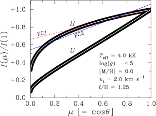
The foregoing numerical methods can (and do) yield substantially different LDC values, even for the standard linear and quadratic representations of a given, fixed, intensity distribution, as is illustrated by Figs. 1 and 2. For a given intensity distribution, in the optical wavelength regime the FC1 $u$ coefficient is usually the smallest numerically; LS2 and FC2 $u$ coefficients are very similar, and relatively large; and the LS1 coefficient is intermediate.

When characterizing model-atmosphere results, the density and distribution of angles at which intensities are calculated, and the weighting scheme, will also influence the numerical values of limb-darkening coefficients (e.g., Díaz-Cordovés & Giménez, 1992; Claret, 2008). In the present work, intensities were computed for $\mu=0.001$ to 1 at steps of 0.001, and equally weighted when fitting functional forms.

Of course, the physics used in constructing the model atmosphere is also critical. The limb-darkening coefficients used throughout this paper were computed using the Atlas9 line-blanketed LTE model-atmosphere code (Kurucz, 1993), as ported to gnu-linux systems by Sbordone, Bonifacio & Castelli (2007), with the Opacity Distribution Functions described by Howarth (2011). Solar abundances, a microturbulent velocity of $v_{\rm t}=2$ km s^-1, and mixing-length parameter $\ell/H=1.25$ were adopted unless noted otherwise. These models use time-independent, plane-parallel structures; while atmospheric extension is unlikely to be important in the parameter space discussed here, the neglect of time-dependent 3D effects may be significant when comparing with empirical results (e.g., Bigot et al. 2006).

Figure 3: Photometrically determined linear limb-darkening coefficients (small dots), for fixed input limb darkening, in the Johnson-Cousins-Glass UVIHL passbands (cf. Section 3.1). Larger symbols show corresponding linear limb-darkening coefficients determined directly from the same input model-atmosphere intensity distributions using flux-conserving and flux-conserving least-squares fitting (FC1, large squares, FC2, large diamonds; Section 2.2. These single-valued results are plotted at arbitrary impact parameters).

Figure 4: Photometrically determined quadratic limb-darkening coefficients for a 4 kK model in the Johnson-Cousins-Glass UVIHL passbands. Left-hand panels, $u_{1},u_{2}$ coefficients (eqtn. 2); right-hand panels, rotated $w_{1},w_{2}$ coefficients (Section 3.2). Larger dots show corresponding quadratic limb-darkening coefficients determined directly from the same input model-atmosphere intensity distributions using flux-conserving and flux-conserving least-squares fitting (FC1, large squares, FC2, large diamonds; Section 2.2. These single-valued results are plotted at arbitrary impact parameters).

Figure 5: Quadratic limb-darkening coefficients determined by Kipping & Bakos (2011a, b) from Kepler photometry compared with model-atmosphere results. Panels are identified by star name, $T_{\rm eff}$, and $\log{g}$. Bands of grey points show the projection onto the ($u_{1},u_{2}$) plane of the 90% of MCMC results yielding the smallest $\chi^{2}$ values, which overlay the best 95% results (black points, not visible in all frames because this figure is a projection of multiparameter modelling onto a specific 2D plane). Green squares show the median values from MCMC runs (the solutions adopted by Kipping & Bakos 2011a, b), and green diamonds the minimum-$\chi^{2}$ MCMC results. Red dots show fits to model-atmosphere intensities (left to right: FC2/LS2 [indistinguishable at this scale], LS1, FC1), while horizontal and vertical lines indicate the SPAM solutions. The small rectangle shown in each panel (perhaps most easily seen by zooming in on the on-line version) encompasses the SPAM solutions for all six targets, and is included to provide an qualitative indication of the rather small scale of uncertainties likely to result from any plausible errors in input stellar parameters. The rotated $w_{1},w_{2}$ axes (eqtn. 6) are shown in the TrES-2 panel, for reference; by design, most of the variance in the MCMC results is in $w_{1}$.

Figure 6: Comparison of linear limb-darkening coefficients determined observationally for HD 209458 (lower set of black points, from Southworth 2008) and SPAM calculations (upper set of red points). The ‘error bars’ on the model-atmosphere results are the result of varying input stellar parameters (see Section 4.2 for details); for both SPAM and empirical results, the error bars are smaller than the points at most wavelengths. Continuous and dotted lines connect LS2 and FC1 model-atmosphere results, respectively.

Figure 7: Comparison of quadratic limb-darkening coefficients for HD 209458. Black points with error bars, empirical values from Southworth (2008); red points, SPAM results (Section 4.2). Continuous and dotted lines connect LS2 and FC1 model-atmosphere results, respectively.

3 Inferences from exotransit photometry

The dispersion in coefficient values introduced simply by numerical techniques poses the question: which procedure is most appropriate for comparing model-atmosphere results with observational determinations of limb darkening? To answer this question it is necessary first to examine just what it is that is measured from transit observations.

Photometric observations of exoplanetary transits record, essentially, the variation of $I_{\lambda}(r)/F_{\lambda}$ along a chord. In practice, this variation is parameterized by an analytical limb-darkening law, whose coefficients are optimized as part of the global fitting procedure. This optimization process is quite different from fitting a limb-darkening law to model-atmosphere intensities, so it is immediately clear that there cannot be any simple one-to-one correspondence between photometric and model-atmopshere LDCs.

Moreover, the extent to which a transit light-curve encodes the global limb darkening must depend on the impact parameter; on how faithfully the chosen parametrization of the limb darkening matches the intensities on those parts of the star that are occulted; and how well it extrapolates to those parts that are not. Given that simple linear and quadratic limb-darkening laws give only approximate representations of actual intensity distributions, it might be anticipated that LD coefficients determined from light-curves must, at some level, suffer systematic biasses depending on impact parameter, reinforcing the point that these photometric coefficients must fail to correspond directly to any equivalent, single-valued, characterization of model-atmosphere results.

To demonstrate and quantify these effects, model transit light-curves were first generated for a range of stellar temperatures and passbands. Limb darkening was represented in the light-curve calculations by eqtn. 3, with coefficients determined by least squares (i.e., for practical purposes, the model-atmosphere results were represented almost exactly). The geometry was set by choosing a ratio of planetary to stellar radii of 1:10 and a centres-of-mass separation of 10$R_{*}$, representative of ‘hot Jupiter’ systems commonly observed to transit (although the subsequent limb-darkening results are insensitive to the adopted values), with the impact parameter varied over the range 0–0.95.

The resulting light-curves were then solved for basic geometrical parameters, and for linear or quadratic LDCs. These calculations were performed using a modified version of jktebop (Southworth et al., 2004a, b), which is itself based on Etzel’s ebop code (Etzel, 1981; Popper & Etzel, 1981). Proximity effects (tidal distortion, ‘reflection’, etc.) were throughout assumed to be negligible.

3.1 Linear law

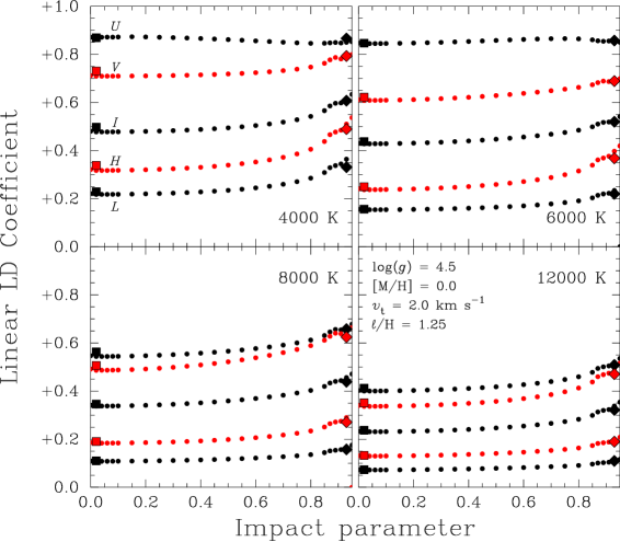
Figure 3 shows a selection of the results, and demonstrates that, in this parameter space, linear LDCs derived from photometry systematically increase with increasing impact parameter, by up to $\sim$0.2 ($\sim$60%). This behaviour is straightforward to understand: in the optical regime $\partial{I}/\partial{\mu}$ decreases with increasing $\mu$, so that any transit that is not central (i.e., inclination $i\neq 90^{\circ}$) samples a relatively steep part of the limb-darkening law. A linear approximation to that law must therefore yield a linear limb-darkening coefficient that is, in general, larger than that derived from a central transit.

Figure 2 illustrates this point by showing model-atmosphere results, and linear approximations, for a 4 kK model. The intensity in the U band is very nearly a linear function of $\mu$, so any characterization will yield similar numerical values for the $u$ coefficient. This is confirmed both in that least-squares and flux-conserving approaches yield similar results in this passband, and in that the $u$ coefficient derived photometrically is insensitive to impact parameter (upper-left panel of Fig. 3). This contrasts with H-band results; the intensity there is a strongly non-linear function of angle, and any diagnostic that characterizes only small $\mu$ values must yield a larger $u$ coefficient than that characterizing the entire centre-to-limb variation. Fig. 3 shows this to be the case.

Fig. 3 also shows the linear limb-darkening coefficients obtained by fitting the input intensity distributions directly, using flux-conserving (FC1) and flux-conserving least-squares (FC2) techniques, which bracket the range of numerical values derived directly from the model atmospheres. In this parameter space, these coefficients also almost bracket the corresponding photometric LDCs which suggests a simple, if rough-and-ready, means of comparing observational and model-atmosphere parametrizations. Furthermore, if one had to choose a single, linear limb-darkening coefficient to compare with photometric results, then the FC1 value is probably the least poor option; for randomly inclined orbits, smaller impact parameters are more probable than larger ones (and observational selection effects also favour higher orbital inclinations), and photometrically determined limb darkening coefficients are generally closest to the FC1 LDC in this case.

3.2 Quadratic law

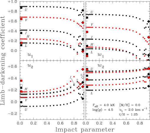
The variations in linear limb-darkening coefficient are present a fortiori for the quadratic coefficients, although here the interpretation is less straightforward because of the well-known strong correlation between $u_{1}$ and $u_{2}$, evident in the left-hand panels of Fig. 4 (see also Fig. 2 in Southworth 2008). Pál (2008) and Kipping & Bakos (2011a) point out that this correlation is largely removed through a rotation onto new principal axes,

$$w_{1} =u_{1}\cos\phi-u_{2}\sin\phi,$$

$$w_{2} =u_{2}\cos\phi+u_{1}\sin\phi,$$ (6)

with $\phi\simeq 40^{\circ}$. Results rotated to these co-ordinates are shown in the right-hand panel of Fig. 4, and confirm that, while the $w_{1}$ values continue to show a large variation with impact parameter, $w_{2}$ is more nearly constant.

The correspondence between the photometric and model-atmosphere results is less straightforward than with the linear law; the model-atmosphere representations of limb darkening show no simple relationship to the photometrically-determined equivalents (notwithstanding rough quantitative similarities). Nevertheless, the small dispersion found for the $w_{2}$ coefficient in both observational and model-atmosphere characterizations of limb darkening indicates that this should be the parameter of choice when making comparisons.

4 Comparing model-atmosphere and photometric limb-darkening

The foregoing sections emphasize that different characterizations of model-atmosphere results can give quite different numerical results (e.g., Fig. 1); and that light-curve analyses, using, of necessity, approximate limb-darkening ‘laws’, yield LDCs that vary with transit geometry (e.g., Fig. 3). Furthermore, although a given analytical limb-darkening law is adopted in photometric studies, the determination of its coefficients through light-curve modelling is, numerically, fundamentally distinct from the techniques of fitting model-atmosphere intensity distributions discussed in Section 2; that is, comparing photometric and model-atmosphere results is, to an extent, like comparing apples and oranges (but see Sandford 1995; Barone 2000). In order to examine the relationship between empirical, photometric LDCs and theoretical model-atmosphere values, it is therefore necessary to devise a method ensuring a fair comparison.

The most direct way to perform such a ‘like for like’ comparison is to adapt the methods used in Section 3, i.e., to generate model light-curves for well-studied systems, using as inputs the empirically determined geometric parameters, coupled to model-atmosphere intensity distributions (in practice, approximated by eqtn. 3) for the ‘known’ stellar parameters. This synthetic photometry can then be solved for the geometric parameters and LDCs, using the same simplified limb-darkening law adopted in the observational photometric analysis. The resulting hybrid synthetic-photometry/atmosphere-model (SPAM) LDCs can reasonably be compared directly with empirical values.

This approach has been used to investigate two illustrative datasets: the eight stars with Kepler data analysed by Kipping & Bakos (2011a, b), and the multiwavelength study of HD 209458 by Knutson et al. (2007; see also Southworth 2008, Claret 2009). Synthetic light-curves were generated with 1000 data points through transit (phases $\pm$0.05). Statistical errors are not quoted on any results because the analysis is essentially deterministic.

4.1 Kepler targets

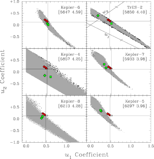
Kipping & Bakos (2011a, b) derived quadratic limb-darkening coefficients for the eight Kepler targets they studied. Their Monte-Carlo Markov-Chain results are reproduced here in Fig. 5.

Custom model atmospheres were computed for each system as described in Section 2.3; adopted stellar parameters are summarized in Table 1 (Appendix A). This group of stars samples a fairly small range in atmospheric properties ($T_{\rm eff}=5647$:$6297$ K, $\log{g}=3.96$:$4.59$, $\mbox{[M/H]}=-0.55$:$+0.33$), which is reflected in a rather small range in model-atmosphere and SPAM LDCs. It’s therefore somewhat surprising that agreement between empirical LDCs and those from the SPAM approach (or from direct fitting to model atmospheres) varies from excellent (Kepler-6) to statistically unacceptable (e.g., Kepler-5).

There is a suggestion that the extent of agreement correlates with temperature; the SPAM LDCs for the three coolest stars fall within the cloud of the best-fitting 90% of solutions, while those for the three hottest lie (just) outside. The trend is for the cloud of empirical values to move towards smaller ($u_{1},u_{2}$) values with increasing temperature, compared to the model-atmosphere results. It’s unclear why the empirical results should show so much greater variation than the models, suggesting that this apparent trend may simply be an artefact of the small sample, or that some additional factor plays an unexpectedly important role.

4.2 HD 209458

Baseline parameters of $T_{\rm eff}=6113$ K (Casagrande et al., 2010), $\log{g}=4.50$, $\mbox{[M/H]}=+0.03$ (Sousa et al., 2008), $v_{\rm t}=2$ km s^-1, $\ell/H=1.25$ were adopted to construct the reference model atmosphere and intensities for HD 209458. Broad-band limb-darkening was calculated by assuming ‘top hat’ response functions for the photometric passbands of the Knutson et al. HST observations. The principal results are summarized in Table 2

Additional models were run for $T_{\rm eff}=5913,6313$; $\log{g}=4.2,4.8$; $\ell/H=0.5$; $v_{\rm t}=0,4~{}\mbox{\rm km$\;$s${}^{-1}$}$; and $\mbox{[M/H]}=-0.4,+0.4$. These ranges allow for quite generous uncertainties in parameters for this well-studied system. The extremes in linear LDCs from the models are for the low-$T_{\rm eff}$ and high-gravity models (numerically largest and smallest coefficients, respectively), and these models are used to illustrate plausible ‘error bars’ on the SPAM coefficients in Figs. 6 and 7.

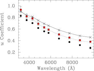
Fig. 6 shows results for linear coefficients. The discrepancies between model-atmosphere and photometric results already noted by Claret (2009; see also Southworth 2008), on the basis of older models, persist in the new analysis.

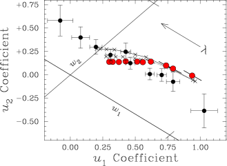
The comparison for quadratic coefficients is shown in Fig. 7. The variation with wavelength of both $u_{1}$ and $u_{2}$ coefficients is much less for the SPAM coefficients than is found empirically. However, both sequences run almost parallel to the rotated $w_{1}$ axis, and agreement in the better-determined $w_{2}$ parameter is tolerable at all wavelengths. In particular, for the $\sim$678 nm passband, which is close to the effective wavelength of the Kepler results, the agreement is reasonably good, [$(w_{1},w_{2})=(0.234,0.385),(0.099,0.363)$ for SPAM and light-curve coefficients, respectively]. This is in contrast to the Kepler results for stars at similar effective temperatures (but is consistent with the result that it is the higher-gravity stars that show the best agreement between models and observations).

5 Summary and conclusions

Different methods of fitting a given limb-darkening law to a given model-atmosphere intensity distribution lead to quite different numerical coefficients. Furthermore, the limb-darkening coefficients determined from photometry of exoplanetary transits are functions of impact parameter, and can’t reliably be compared directly to any of the standard model-atmosphere characterizations.

A more direct comparison can be made if the model intensities are translated into observer space, through the medium of synthetic light-curves. The resulting synthetic-photometry/atmosphere-model (SPAM) limb-darkening coefficients are not single-valued, but can be compared directly with empirical results.

[If one had to choose a traditional single-valued representation of model-atmosphere results, then at optical wavelengths closest agreement with the SPAM results is generally obtained with the standard (FC1) flux-conserving method, which also yields the smallest value of the linear limb-darkening coefficient.]

For the commonly used quadratic limb-darkening law, most of the variation in different fits to model-atmosphere intensities is in the $w_{1}$ parameter, with much smaller dispersions in the $w_{2}$ coefficient. Since the $w_{1}$ axis is also defined as that which maximizes dispersion in observational (Monte-Carlo) results, the most sensitive comparison between models and observations is in $w_{2}$.

New model-atmosphere calculations, analysed with the SPAM approach, show mixed results. Agreement with empirical Kepler LDCs is good in some cases (differences in $w_{2}$ less than 0.06 in four out of six systems), but not in others. There is a hint of a possible temperature dependence in the extent of disagreement for these targets, with cooler stars showing better agreement. However, at similar effective wavelengths HST results for HD 209458 (which is at the hotter end of the range of Kepler targets) agree well with models; there are discrepancies at longer and short wavelengths, though again with fair agreement in $w_{2}$. Since gravity (and metallicity) correlate with temperature for the Kepler sample, and since HD 209458 is both high-temperature and high-gravity in the context of that sample, this might be taken as an indication that agreement is better at higher gravities (with temperature as a secondary factor). However, the ranges in all quantitities characterizing the atmospheres are so small as to render such conclusions speculative at this stage. Forthcoming results from Kepler, and other missions, should enlarge the parameter space, and permit better discrimination of where models and observations do and do not agree.

Appendix A Fit results

Table 1: Limb-darkening results: Kepler photometry. For each star, the physical parameters used in the model-atmosphere calculations are first listed, followed by the resulting 4-parameter Kepler-band limb-darkening coefficients (eqtn. 3). Subsequent columns list the SPAM coefficients, determined by fitting synthetic light-curves generated from the ‘known’ system parameters; the empirical photometric coefficients; and, for reference, coefficients determined directly from the model-atmosphere intensity distributions. All necessary stellar & system parameters are adopted from Kipping & Bakos (2011a, b).

	Photometry	Photometry	Model-atmosphere fits
	(Synthetic)	(Observed)	LS1	LS2	FC1	FC2
Kepler-4	$T_{\rm eff}=5857$ K, $\log{g}=4.25$, $\mbox{[M/H]}=+0.17$, $v_{\rm t}=2$ km s-1, $\ell/H=1.25$.
$a_{n},n=1,4$	+7.63788E-01	$-$7.97285E-01	+1.40090E+00	$-$5.86378E-01
linear, $u$	+0.6080		+0.6252	+0.6491	+0.5828	+0.6491
quad, $u_{1}$	+0.5201	$+0.61^{+0.59}_{-0.39}$	+0.4805	+0.4480	+0.5035	+0.4481
quad, $u_{2}$	+0.1230	$-0.21^{+0.52}_{-0.68}$	+0.1931	+0.2256	+0.1586	+0.2256
Kepler-5	$T_{\rm eff}=6297$ K, $\log{g}=3.96$, $\mbox{[M/H]}=+0.03$, $v_{\rm t}=2$ km s-1, $\ell/H=1.25$.
$a_{n},n=1,4$	+7.34699E-01	$-$7.94487E-01	+1.43212E+00	$-$6.20527E-01
linear, $u$	+0.5564		+0.6011	+0.6265	+0.5566	+0.6267
quad, $u_{1}$	+0.4877	$+0.25^{+0.13}_{-0.12}$	+0.4537	+0.4248	+0.4739	+0.4250
quad, $u_{2}$	+0.1377	$+0.37^{+0.25}_{-0.27}$	+0.1966	+0.2254	+0.1654	+0.2253
Kepler-6	$T_{\rm eff}=5647$ K, $\log{g}=4.59$, $\mbox{[M/H]}=+0.33$, $v_{\rm t}=2$ km s-1, $\ell/H=1.25$.
$a_{n},n=1,4$	+8.20192E-01	$-$9.18046E-01	+1.53037E+00	$-$6.26480E-01
linear, $u$	+0.5967		+0.6436	+0.6664	+0.6025	+0.6665
quad, $u_{1}$	+0.5415	$+0.55^{+0.13}_{-0.11}$	+0.5011	+0.4675	+0.5262	+0.4675
quad, $u_{2}$	+0.1189	$+0.01^{+0.26}_{-0.27}$	+0.1901	+0.2240	+0.1527	+0.2240
Kepler-7	$T_{\rm eff}=5933$ K, $\log{g}=3.98$, $\mbox{[M/H]}=+0.11$, $v_{\rm t}=2$ km s-1, $\ell/H=1.25$.
$a_{n},n=1,4$	+7.48602E-01	$-$7.78844E-01	+1.38072E+00	$-$5.77728E-01
linear, $u$	+0.5850		+0.6205	+0.6439	+0.5790	+0.6440
quad, $u_{1}$	+0.5191	$+0.34^{+0.16}_{-0.13}$	+0.4795	+0.4480	+0.5017	+0.4481
quad, $u_{2}$	+0.1183	$+0.33^{+0.26}_{-0.34}$	+0.1881	+0.2196	+0.1546	+0.2195
Kepler-8	$T_{\rm eff}=6213$ K, $\log{g}=4.28$, $\mbox{[M/H]}=-0.55$, $v_{\rm t}=2$ km s-1, $\ell/H=1.25$.
$a_{n},n=1,4$	+7.13647E-01	$-$7.27611E-01	+1.35455E+00	$-$5.92941E-01
linear, $u$	+0.5817		+0.5980	+0.6240	+0.5525	+0.6241
quad, $u_{1}$	+0.4864	$+0.41^{+0.55}_{-0.25}$	+0.4474	+0.4176	+0.4675	+0.4179
quad, $u_{2}$	+0.1337	$+0.11^{+0.44}_{-0.83}$	+0.2008	+0.2305	+0.1701	+0.2304
TrES-2	$T_{\rm eff}=5850$ K, $\log{g}=4.40$, $\mbox{[M/H]}=+0.15$, $v_{\rm t}=2$ km s-1, $\ell/H=1.25$.
$a_{n},n=1,4$	+6.97192E-01	$-$6.67832E-01	+1.29178E+00	$-$5.62467E-01
linear, $u$	+0.6238		+0.6117	+0.6366	+0.5676	+0.6368
quad, $u_{1}$	+0.4754	$+0.52^{+0.44}_{-0.34}$	+0.4644	+0.4344	+0.4846	+0.4346
quad, $u_{2}$	+0.1608	$+0.06^{+0.37}_{-0.48}$	+0.1964	+0.2264	+0.1659	+0.2264

Table 2: Limb-darkening results: HD 209458. System parameters and observed LDCs are from Southworth (2008). Stellar parameters $T_{\rm eff}=6113$ K (Casagrande et al., 2010), $\log{g}=4.50$, $\mbox{[M/H]}=+0.03$ (Sousa et al., 2008), $v_{\rm t}=2$ km s^-1, $\ell/H=1.25$. Columns follow the model of Table 1, with rows grouped by HST wavelength in nm.

	Photometry	Photometry	Model-atmosphere fits
	(Synthetic)	(Observed)	LS1	LS2	FC1	FC2
HST-320;	$a_{n},n=1,4$	+4.58205E-01	-7.02251E-01	+1.97519E+00	-7.98143E-01
linear, $u$	$+0.9346$	$+0.828{\pm}0.023$	$+0.9064$	$+0.9029$	$+0.9151$	$+0.9029$
quad, $u_{1}$	$+0.9373$	$+1.030{\pm}0.102$	$+0.9438$	$+0.9607$	$+0.9428$	$+0.9607$
quad, $u_{2}$	$-0.0076$	$-0.384{\pm}0.182$	$-0.0500$	$-0.0681$	$-0.0553$	$-0.0681$
HST-375;	$a_{n},n=1,4$	+6.43615E-01	-9.36895E-01	+2.09622E+00	-8.88657E-01
linear, $u$	$+0.8204$	$+0.754{\pm}0.013$	$+0.8283$	$+0.8356$	$+0.8118$	$+0.8356$
quad, $u_{1}$	$+0.7901$	$+0.791{\pm}0.052$	$+0.7809$	$+0.7844$	$+0.7888$	$+0.7844$
quad, $u_{2}$	$+0.0680$	$-0.073{\pm}0.012$	$+0.0632$	$+0.0596$	$+0.0460$	$+0.0596$
HST-430;	$a_{n},n=1,4$	+6.15746E-01	-8.44919E-01	+2.00870E+00	-8.87838E-01
linear, $u$	$+0.7839$	$+0.703{\pm}0.007$	$+0.8005$	$+0.8118$	$+0.7758$	$+0.8118$
quad, $u_{1}$	$+0.7370$	$+0.703{\pm}0.036$	$+0.7283$	$+0.7312$	$+0.7360$	$+0.7312$
quad, $u_{2}$	$+0.1006$	$-0.001{\pm}0.068$	$+0.0964$	$+0.0933$	$+0.0797$	$+0.0933$
HST-485;	$a_{n},n=1,4$	+6.33987E-01	-6.21291E-01	+1.55033E+00	-7.10907E-01
linear, $u$	$+0.6919$	$+0.618{\pm}0.006$	$+0.7276$	$+0.7482$	$+0.6865$	$+0.7483$
quad, $u_{1}$	$+0.6197$	$+0.612{\pm}0.034$	$+0.5962$	$+0.5826$	$+0.6109$	$+0.5826$
quad, $u_{2}$	$+0.1418$	$+0.009{\pm}0.062$	$+0.1754$	$+0.1894$	$+0.1511$	$+0.1894$
HST-540;	$a_{n},n=1,4$	+7.10040E-01	-7.19161E-01	+1.47157E+00	-6.49635E-01
linear, $u$	$+0.6307$	$+0.561{\pm}0.007$	$+0.6684$	$+0.6919$	$+0.6248$	$+0.6919$
quad, $u_{1}$	$+0.5578$	$+0.426{\pm}0.039$	$+0.5240$	$+0.4999$	$+0.5437$	$+0.5000$
quad, $u_{2}$	$+0.1364$	$+0.248{\pm}0.092$	$+0.1927$	$+0.2171$	$+0.1622$	$+0.2171$
HST-580;	$a_{n},n=1,4$	+7.20922E-01	-6.88211E-01	+1.34528E+00	-5.92544E-01
linear, $u$	$+0.5917$	$+0.534{\pm}0.006$	$+0.6322$	$+0.6583$	$+0.5852$	$+0.6584$
quad, $u_{1}$	$+0.5141$	$+0.462{\pm}0.036$	$+0.4756$	$+0.4453$	$+0.4967$	$+0.4455$
quad, $u_{2}$	$+0.1417$	$+0.126{\pm}0.063$	$+0.2089$	$+0.2394$	$+0.1770$	$+0.2393$
HST-678;	$a_{n},n=1,4$	+7.67414E-01	-7.43741E-01	+1.22290E+00	-5.25063E-01
linear, $u$	$+0.5090$	$+0.437{\pm}0.006$	$+0.5520$	$+0.5824$	$+0.5011$	$+0.5826$
quad, $u_{1}$	$+0.4267$	$+0.309{\pm}0.037$	$+0.3799$	$+0.3392$	$+0.4044$	$+0.3395$
quad, $u_{2}$	$+0.1442$	$+0.214{\pm}0.061$	$+0.2295$	$+0.2696$	$+0.1935$	$+0.2695$
HST-775;	$a_{n},n=1,4$	+7.82449E-01	-7.91226E-01	+1.16704E+00	-4.88230E-01
linear, $u$	$+0.4545$	$+0.377{\pm}0.008$	$+0.4964$	$+0.5282$	$+0.4458$	$+0.5286$
quad, $u_{1}$	$+0.3737$	$+0.197{\pm}0.047$	$+0.3240$	$+0.2785$	$+0.3494$	$+0.2790$
quad, $u_{2}$	$+0.1384$	$+0.299{\pm}0.078$	$+0.2299$	$+0.2741$	$+0.1929$	$+0.2739$
HST-873;	$a_{n},n=1,4$	+7.95398E-01	-8.55463E-01	+1.17721E+00	-4.90744E-01
linear, $u$	$+0.4088$	$+0.324{\pm}0.011$	$+0.4498$	$+0.4837$	$+0.3996$	$+0.4838$
quad, $u_{1}$	$+0.3259$	$+0.079{\pm}0.069$	$+0.2751$	$+0.2289$	$+0.3030$	$+0.2290$
quad, $u_{2}$	$+0.1396$	$+0.400{\pm}0.114$	$+0.2331$	$+0.2774$	$+0.1930$	$+0.2773$
HST-971;	$a_{n},n=1,4$	+7.63034E-01	-7.89085E-01	+1.07318E+00	-4.49903E-01
linear, $u$	$+0.3835$	$+0.275{\pm}0.016$	$+0.4242$	$+0.4588$	$+0.3732$	$+0.4591$
quad, $u_{1}$	$+0.2997$	$-0.078{\pm}0.098$	$+0.2496$	$+0.2021$	$+0.2753$	$+0.2025$
quad, $u_{2}$	$+0.1398$	$+0.581{\pm}0.164$	$+0.2330$	$+0.2782$	$+0.1958$	$+0.2780$

Appendix B Systematics of geometric parameters

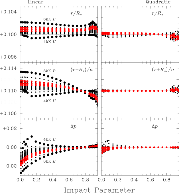
Because light-curves have only a rather weak dependence on limb darkening, we might expect that the use of simplified limb-darkening laws, or even moderately inaccurate LDCs, should have only a very modest effect on the determination of basic geometric parameters when modelling photometry. To demonstrate this (at the referee’s suggestion), additional results from the model grids described in Section 3 are presented in Fig 8.

[To remind the reader, model light-curves were generated using a ratio of planetary to stellar radii of 1:10 and a centres-of-mass separation of 10$R_{*}$, over a range of impact parameters, and an effectively exact representation of limb darkening. These light-curves were then solved, adopting linear or quadratic limb darkening (with the LDCs as free parameters). It is the results of these light-curve solutions that are summarized in Fig 8.]

The systematic errors in fitted geometric parameters (up to $\sim$4% in $r/R_{*}$ and $(r+R_{*})/a$ for the models presented here) might be significant for the best-quality photometry if a linear limb-darkening law is assumed, but are negligible if a quadratic law is used.

Figure 8: Geometric parameters determined from modelling synthetic light-curves, as functions of input impact parameter. The light-curves were generated using essentially exact representations of limb darkening; ratio of planetary to stellar radii $r/R_{*}=0.1$; the sum of the radii, in units of the semi-major axis $r+R_{*})/a=0.11$. Light-curve solutions assume linear (left-hand panels) or quadratic (right-hand panels) limb darkening, with coefficients optimised as part of the fitting process. The (generally small) departures from input parameters are solely a result of using these approximate representations of limb darkening. Results are shown for stellar models at 4, 6, 8, and 12 kK, and UBVRIJHKL passbands; 4-kK U-band and 8-kK B-band results bracket most of the data when a linear law is adopted, and are highlighted with larger symbols. Results for the R band, which are representative of typical unfiltered CCD systems, are shown in red.

References

- Aufdenberg, Ludwig & Kervella (2005) Aufdenberg, J.P., Ludwig, H.-G., Kervella, P., 2005, ApJ, 633 , 424
- Barone (2000) Barone, J.E., 2000, Brit. Medical J., 321, 1569
- Bigot et al. (2006) Bigot, L., Kervella, P., Thévenin, F., Ségransan, D., 2006, A&A, 446, 635
- Casagrande et al. (2010) Casagrande, L., Ramírez, I., Meléndez, J., Bessell, M., Asplund, M., 2010, A&A, 512, 54
- Claret (2000) Claret, A., 2000, A&A, 363, 1081
- Claret (2008) Claret, A., 2008, A&A, 482, 259
- Claret (2009) Claret, A., 2009, A&A, 506, 1335
- Díaz-Cordovés & Giménez (1992) Díaz-Cordovés, J., Giménez, A., 1992, A&A, 259, 227
- Dominik (2004) Dominik, M., 2004, MNRAS, 352, 1315
- Etzel (1981) Etzel, P. B., 1981, in Carling, E. B., Kopal, Z., eds, NATO ASI Ser. C, 69, Photometric and Spectroscopic Binary Systems. Dordrecht, p. 111
- Howarth (2011) Howarth, I.D., 2011 MNRAS, 413, 1515
- Kipping & Bakos (2011a) Kipping, D., Bakos, G., 2011a, ApJ, 730, 50
- Kipping & Bakos (2011b) Kipping, D., Bakos, G., 2011b, ApJ, 733, 36
- Knutson et al. (2007) Knutson, H.A., Charbonneau, D., Noyes, R.W., Brown, T.M., Gilliland, R.L., 2007, ApJ, 655, 564
- Kopal (1949) Kopal, Z., 1949, HCO Circ. 454
- Kurucz (1993) Kurucz, R.L., 1993, CD-ROM 12, Smithsonian Astrophysical Observatory
- Mandel & Agol (2002) Mandel, K., Agol, E., 2002, ApJ, 580, L171
- Milne (1921) Milne E.A., 1921, MNRAS 81, 361
- Pál (2008) Pál, A., 2008, MNRAS, 390, 281P
- Popper & Etzel (1981) Popper, D.M., Etzel, P.B., 1981, ApJ, 86, 102
- Sbordone, Bonifacio & Castelli (2007) Sbordone, L., Bonifacio, P., Castelli, F., 2007, in Convection in Astrophysics (IAU Symp. 239), p. 71
- Sandford (1995) Sandford, S.A., 1995, Annals of Improbable Research, 1, (3)
- Schwarzschild (1906) Schwarzschild K., 1906, Nachrichten von der Gesellschaft der Wissenschaften zu Göttingen, Mathematisch-Physikalische Klasse, p. 43
- Sousa et al. (2008) Sousa, S.G., Santos, N.C., Mayor, M., Udry, S., Casagrande, L., Israelian, G., Pepe, F., Queloz, D., Monteiro, M.J.P.F.G., 2008, A&A, 487, 373
- Southworth et al. (2004a) Southworth, J., Maxted, P.F.L., Smalley, B., 2004a, MNRAS, 351, 1277
- Southworth et al. (2004b) Southworth, J., Zucker, S., Maxted, P.F.L., Smalley, B., 2004b, MNRAS, 355, 986
- Southworth (2008) Southworth, J., 2008, MNRAS, 386, 1644
- Wade & Rucinski (1985) Wade, R.A., Rucinski, S.M., 1985, A&AS, 60, 471
- Witt (1995) Witt, H.J., 1995, ApJ, 449, 42
- Zub et al. (2011) Zub, M., Cassan, A., Heyrovský, D., Fouqué, P., Stempels, H.C., et al., 2011, A&A, 525, 15