Determining $R$-parity violating parameters from neutrino and LHC data

Abstract

In supersymmetric models neutrino data can be explained by $R$-parity violating operators which violate lepton number by one unit. The so called bilinear model can account for the observed neutrino data and predicts at the same time several decay properties of the lightest supersymmetric particle. In this paper we discuss the expected precision to determine these parameters by combining neutrino and LHC data and discuss the most important observables. We show that one can expect a rather accurate determination of the underlying $R$-parity parameters assuming mSUGRA relations between the $R$-parity conserving ones and discuss briefly also the general MSSM as well as the expected accuracies in case of a prospective $e^{+}e^{-}$ linear collider. An important observation is that several parameters can only be determined up to relative signs or more generally relative phases.

I Introduction

With the start of the LHC the exploration of the terascale has begun and, thus, in the search for extensions of the Standard Model (SM) significant higher mass scales can be tested as in the past. Supersymmetry (SUSY) is among the most favoured candidates as it allows for example the unification of gauge couplings and stabilizes the hierarchy of the Planck scale (or the GUT scale) and the electroweak scale. Once supersymmetry has been found, there will be two main tasks: (i) to determine the underlying parameters of the model and (ii) to check if the minimal model is realized in nature or an extended one.

In principle one can supersymmetrize all known mechanisms to generate neutrino masses and mixing angles, see e. g. ref. Nath et al. (2010). However, supersymmetry offers an intrinsic possibility to generate neutrino masses, namely $R$-parity violation (RPV), for an review see e. g. Hirsch and Valle (2004). In this case neutrino masses are generated either via mixing with neutralinos or via loop effects Hall and Suzuki (1984); Hempfling (1996); Nardi (1997). We will be constraining ourself to bilinear R-parity violation (BRpV) Kaplan and Nelson (2000); Hirsch et al. (2000); Diaz et al. (2003a), thus breaking lepton number but not baryon number. This model can be viewed as the effective theory of a spontaneously broken $R$-parity Santamaria and Valle (1987); Romao and Valle (1992); Nilles and Polonsky (1997); Kitano and Oda (2000). The BRpV neutrino mass model has only a few free parameters and therefore is very predictive. Furthermore, in contrast to trilinear RPV neutrino mass models, the constraints from LEP on the $R$-parity violating couplings are automatically satisfied as the couplings are small due to the requirement of explaining correctly neutrino data.

The RPV couplings giving rise to neutrino masses are also responsible for the decay properties of the neutralino. Therefore, an important smoking gun signal for these models is the strong connection between neutralino physics and neutrino mixing parameters. Some ratios of the branching ratios of the neutralino, or more generally the lightest supersymmetric particle, are related to neutrino mixing angles Mukhopadhyaya et al. (1998); Porod et al. (2001); Hirsch et al. (2002); Hirsch and Porod (2003). In particular, approximately the same number of muons as taus are expected along with a $W$-boson because their ratio is given by tangent of the nearly maximal atmospheric mixing angle. By measuring the decay properties of the neutralino, which is likely to be done by the LHC, a severe test of this model is possible.

Due to the smallness of the RPV couplings the neutralino will have a long lifetime, but short enough for it to mainly decay within the detectors at the LHC. The prospects for collider discovery of RPV, responsible for the neutrino masses and mixings, in mSUGRA have been thoroughly studied Barger et al. (2002); Magro et al. (2003); de Campos et al. (2005a, 2008a); De Campos et al. (2010).

Once this scenario is confirmed an important question will be how well the underlying parameters can be determined. There have been several studies within the MSSM with conserved $R$-parity Blair et al. (2001, 2003); Bechtle et al. (2006); Lafaye et al. (2008); Bechtle et al. (2010); Adam et al. (2011); Hirsch et al. (2011). In this paper we want to focus on the determination of the RPV parameters taking into account neutrino and LHC data. We will focus on a specific scenario for the details but comment on how this can be extrapolated to others. We will also work out which are the most sensitive observables.

This paper is organized as follows: in the next section we will recall briefly the main features of the BRpV model. In Section III we discuss the details of the fit procedure and present the fit results in Section IV and then draw in Section V our conclusions.

II Explicit bilinear $R$-parity violation

The MSSM with explicit bilinear $R$-parity violation is specified by the superpotential Diaz et al. (1998)

$$\mathcal{W}_{\mathrm{BRpV}}=\mathcal{W}_{\mathrm{MSSM}}+\epsilon_{i}\widehat{L}_{i}\widehat{H}_{u}\,,$$ (1)

where the last term explicitly violates both $R$-parity and lepton number in all three generations. In addition one has to add corresponding terms to the soft SUSY breaking potential,

$$V_{\mathrm{soft}}^{\mathrm{BRpV}}=V_{\mathrm{soft}}^{\mathrm{MSSM}}+B_{i}\epsilon_{i}\tilde{L}_{i}H_{u}\,,$$ (2)

which induce vacuum expectation values (VEVs) $v_{i}\mathrel{\mathop{:}\!\!=}\Braket{\tilde{\nu}_{i}}$ for the sneutrinos. Using the tadpole equations one can take the sneutrino VEVs as input instead of the $B_{i}$ Hirsch and Valle (2004).

One important aspect of this model is that the $R$-parity breaking terms give rise to mixings between SM and SUSY particles. In the neutral fermion sector the mixing between neutralinos and neutrinos leads to one massive neutrino at tree-level while the other two neutrinos acquire masses through loop corrections Hirsch et al. (2000); Diaz et al. (2003a); Hirsch and Valle (2004). The effective neutrino mass matrix at tree- and one-loop level is given by

$$(m_{\mathrm{eff,LO}})_{ij} =a\Lambda_{i}\Lambda_{j}$$ (3)

$$(m_{\mathrm{eff,NLO}})_{ij} =b\Lambda_{i}\Lambda_{j}+c(\Lambda_{i}\epsilon_{j}+\epsilon_{i}\Lambda_{j})+d\epsilon_{i}\epsilon_{j}\,,$$ (4)

where $a$, $b$, $c$, $d$ are functions of $R$-parity conserving parameters and $\Lambda_{i}$ are the so called alignment parameters

$$\Lambda_{i}=\mu v_{i}+v_{d}\epsilon_{i}\,.$$ (5)

For example $a$ is given by

$$a=\frac{-(g^{2}M_{1}+g^{\prime}{}^{2}M_{2})}{\sqrt{\Pi_{j=1}^{4}m_{\tilde{\chi}^{0}_{j}}}}$$ (6)

and $b$ is equal to $a$ plus radiative corrections. From the mixing matrix that diagonalizes eq. (4) one obtains expressions for the neutrino mixing angles in terms of the $R$-parity breaking parameters which can approximately be expressed as Hirsch et al. (2000); Diaz et al. (2003a):

$$\tan^{2}\theta_{23}\approx\left(\frac{\Lambda_{2}}{\Lambda_{3}}\right)^{2}\,,\qquad\tan^{2}\theta_{13}\approx\frac{\Lambda_{1}^{2}}{\Lambda_{2}^{2}+\Lambda_{3}^{2}}\,,\qquad\tan^{2}\theta_{12}\approx\left(\frac{\widetilde{\epsilon_{1}}}{\widetilde{\epsilon_{2}}}\right)^{2}\,,$$ (7)

where $\widetilde{\epsilon_{i}}=V_{\mathrm{tree},ij}\epsilon_{j}$ and $V_{\mathrm{tree}}$ diagonalizes the tree-level neutrino mass matrix eq. (3). As one can see from eqs. (4) and (7) both the neutrino masses and the mixing angles are predicted in terms of the $R$-parity breaking parameters. It turns out that the approximation for $\tan^{2}\theta_{23}$ is relative insensitive when going from tree-level to one-loop level. The one for $\tan^{2}\theta_{13}$ can be quite sensitive to loop corrections, in particular if $\epsilon_{2}\Lambda_{2}\epsilon_{3}\Lambda_{3}>0$. Hirsch et al. (2000); Diaz et al. (2003a). This will also manifest itself later in the fits discussed in Section IV. The most important loop contributions are due to sbottom-bottom and stau-tau loops Hirsch et al. (2000); Diaz et al. (2003a) which are in both cases proportional to $\epsilon_{j}\epsilon_{k}/|\mu|^{2}$. However, there are also regions in parameter space where the mixing between sleptons and the charged Higgs boson Diaz et al. (2003a) and/or the sneutrino-neutrino loops give large contributions Dedes et al. (2006).

The violation of $R$-parity also implies that the lightest supersymmetric particle (LSP), which we assume to be the lightest neutralino here, is no longer stable and typically decays inside the detector once the parameters are adjusted to satisfy the neutrino constraints Porod et al. (2001); Hirsch et al. (2002); Hirsch and Porod (2003); Hirsch et al. (2005). The parameters that determine the decay properties of the LSP are the same parameters that lead to neutrino masses and oscillation which implies that there are correlations between the neutralino branching ratios and the neutrino mixing angles Mukhopadhyaya et al. (1998); Porod et al. (2001), e. g.

$$\frac{\mathrm{BR}(\tilde{\chi}^{0}_{1}\to W^{\pm}\mu^{\mp})}{\mathrm{BR}(\tilde{\chi}^{0}_{1}\to W^{\pm}\tau^{\mp})}\approx\tan^{2}\theta_{23}$$ (8)

This can be most easily seen by performing first an approximate diagonalization of the chargino and neutralino mass matrices as in Hirsch and Valle (1999). The parts of the corresponding mixing matrices responsible for the mixing between neutrinos and neutralinos as well as charged leptons and charginos can be expressed in terms of

$$\frac{\epsilon_{i}}{\mu}\,,\hskip 5.69054pt\frac{\Lambda_{i}}{\sqrt{\Pi_{j=1}^{4}m_{\tilde{\chi}^{0}_{j}}}}\,,\hskip 5.69054pt\frac{\Lambda_{i}}{m_{\tilde{\chi}^{+}_{1}}m_{\tilde{\chi}^{+}_{2}}}\,.$$ (9)

and enter also the corresponding couplings in the decays used in eq. (8). Moreover, the decay length of the LSP is proportional to the $R$-parity breaking parameters Porod et al. (2001); de Campos et al. (2005a); De Campos et al. (2010). All these facts can be used to determine these parameters once information on the $R$-parity conserving ones is available.

III Fit Procedure

LHC will provide first information on the SUSY parameters once the corresponding signals are observed. However, it will be unlikely that the complete spectrum will be discovered and, thus, the first parameter fits will be performed within specific high scale models Bechtle et al. (2006); Lafaye et al. (2008); Bechtle et al. (2010); Adam et al. (2011). Therefore, the fits presented in this paper are performed in mSUGRA models which are augmented by bilinear $R$-parity breaking parameters at the electroweak scale. These models therefore have eleven free parameters, namely the five mSUGRA parameters $m_{0}$, $M_{1/2}$, $A_{0}$, $\tan\beta$, and $\Sign{\mu}$ and the six bilinear $R$-parity breaking parameters $\epsilon_{i}$, and $\Lambda_{i}$ (or $v_{i}$ respectively). For the theoretical predictions of the neutrino oscillation data, the LSP decay properties, and LHC/ILC observables, SPhenoPorod (2003) version 3.0.beta54 has been used.

In order to measure the agreement between the data and the model for a particular choice of parameters a simple $\chi^{2}$ function is used,

$$\chi^{2}(\bm{a})=\sum_{i}\left(y_{i}-f_{i}(\bm{a})\right)^{2}/\sigma_{i}^{2}\,,$$ (10)

where the $y_{i}$ are data points with their associated uncertainties or experimental errors $\sigma_{i}$ and the $f_{i}(\bm{a})$ are theoretical predictions for these data points at the point $\bm{a}$ in parameter space. The data points used for the fits were also calculated by SPheno for a specific mSUGRA point, where the $R$-parity breaking parameters are not explicitly specified but are calculated iteratively such that the predicted neutrino mixing angles and squared mass differences lie in the $3\sigma$ confidence region as given in (Schwetz et al., 2008, Table A1). If the $R$-parity breaking parameters as determined by SPheno are denoted by $\bm{\widehat{a}}$, then the data points are equal to their predictions at the point $\bm{\widehat{a}}$ where the $R$-parity breaking parameters are explicitly specified, i. e. $y_{i}=f_{i}(\bm{\widehat{a}})$.

Since the data points used in the fits are themselves theoretical predictions, the absolute minimum of eq. (10) is trivially given by $\chi^{2}_{\mathrm{min}}\mathrel{\mathop{:}\!\!=}\chi^{2}(\bm{\widehat{a}})=0$. Instead of finding the parameter point with the best goodness of fit, the purpose of data fitting is then to estimate the parameter errors based on the uncertainties $\sigma_{i}$, or to locate other minima in a multimodal $\chi^{2}$-landscape that have equally good $\chi^{2}$-values. In order to find all minima in a specific region of parameter space and to determine the boundaries of $\chi^{2}(\bm{a})$ for the error estimation, the Minuit MigradJames and Roos (1975) optimization algorithm was used repeatedly at random starting points in parameter space. This procedure gives a good coverage of the $\chi^{2}$-landscape and finds with high probability all minima which lie in the region that is bounded by the starting points. As interface between SPheno and Minuit the general purpose fitting program Kaimini, which provides different deterministic and stochastic optimization algorithms and works with any program that implements the SUSY Les Houches Accord (SLHA)Allanach et al. (2009); Skands et al. (2004), is used.

IV Results

IV.1 Fit Setup

Various fits with different free parameters and data points were carried out. The following subsections discusses fits where the $R$-parity breaking parameters are free parameters and different observables that depend on these parameters (that are the neutrino oscillation data and the $\tilde{\chi}^{0}_{1}$ decay properties) are used as data points. For each of these combinations three fits are performed which differ with respect to the mSUGRA parameters being fixed or free parameters of the fit and the set of corresponding data points. In the first setup the mSUGRA parameters are fixed and only the neutrino and/or neutralino observables are used as data points. In the second and third setup the mSUGRA parameters $m_{0}$, $M_{1/2}$, $A_{0}$ and $\tan\beta$ are free parameters in addition to the $R$-parity breaking parameters. The additional data points of the second setup are the “edge variables” $(m^{2}_{ll})^{\mathrm{edge}}$, $(m^{2}_{qll})^{\mathrm{edge}}$, $(m^{2}_{qll})^{\mathrm{thres}}$, $(m^{2}_{bll})^{\mathrm{thres}}$, $(m^{2}_{ql})_{\mathrm{min}}^{\mathrm{edge}}$, and $(m^{2}_{ql})_{\mathrm{max}}^{\mathrm{edge}}$, where the predicted relative uncertainties were taken from (Weiglein et al., 2006, Table 5.13). This setup is denoted as “LHC”. The third setup includes in addition to the edge variables the masses of the $\tilde{\chi}^{0}_{i}$, $\tilde{\chi}^{\pm}_{i}$, sleptons, and the $\tilde{t}_{1}$ assuming that are measured at a prospective future $e^{+}e^{-}$ linear collider such as ILC or CLIC. The relative uncertainties of these observables were taken from (Weiglein et al., 2006, Table 5.14). This setup is denoted as “LHC+ILC”. To be conservative the total uncertainties in both setups were obtained by summing statistic and systematic uncertainties linearly. We note, that taking the relative uncertainties for the collider observables equal for different points of parameter space is a strong assumption which would have to be confirmed by individual studies which are however not available in the literature. However, as we will see below the uncertainties on the RPV parameters are dominated by the uncertainties of the measurements of neutralino decay branching ratios and that the uncertainties on the measurements of masses and edge variables are only sub-dominant.

Fits for the various setups were performed for different SUSY benchmark points, including SPS 1a^′ Aguilar-Saavedra et al. (2006), 1a, 1b, and 3 Allanach et al. (2002). In this paper we discuss in detail as a typical example SPS 1a^′ working out the main features as most experimental studies for the collider observables used have been performed for points close by and, thus, the assumption of using the same relative uncertainties can be more easily justified. The results for the other study points and additional plots for SPS 1a^′ are given on our web page Thomas . We are aware that SPS 1a^′ is potentially excluded by recent LHC data Khachatryan et al. (2011); Aad et al. (2011) although the corresponding searches have been performed for the $R$-parity conserving case. However, we have checked that qualitative features do not depend on the point under study, e. g. they are the same for SPS 3 which is not excluded by existing data.

IV.2 Neutrino oscillation data

The free parameters of these fits are the six $R$-parity breaking parameters while the data points are the neutrino oscillation data, which are the two mass squared differences $\Delta m^{2}_{\mathrm{atm}}$ and $\Delta m^{2}_{\mathrm{sol}}$ and the three mixing angles $\tan^{2}\theta_{\mathrm{atm}}$, $\tan^{2}\theta_{\mathrm{sol}}$, and $\sin^{2}\theta_{13}$. As uncertainties for the data points the mean value of the upper and lower $1\sigma$ errors from Table A1 of Schwetz et al. (2008) were used. To get meaningful results from the fits, the number of degrees of freedom, which is the number of data points minus the number of parameters, must be equal to or greater than zero. Therefore the $\tilde{\chi}^{0}_{1}$ decay width was used as additional data point and we assumed that it can be measured with an accuracy of $15\text{\,}\%$ Ros . We perform this fit separately to get an understanding how the different sectors contribute to a global fit.

Figure 1: Likelihood maps of fits at SPS 1a^′ for various parameter combinations using neutrino data and the neutralino decay width: $\epsilon_{1}$-$\epsilon_{2}$ (upper left), $\bm{\epsilon}^{2}$-$|\bm{\Lambda}|$ (upper right), $\Lambda_{1}$-$\Lambda_{3}$ (lower left) and $\Lambda_{2}$-$\Lambda_{3}$ (lower right). These maps are projections of the six-dimensional parameter space onto the corresponding planes such that points with a higher likelihood cover points with a lower likelihood. The regions with maximum likelihood (which are colored black) correspond to minimal $\chi^{2}$-values. See section IV.2 for further details.

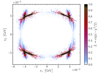
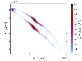
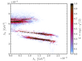
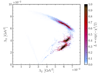
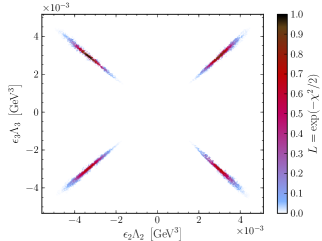
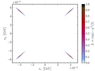
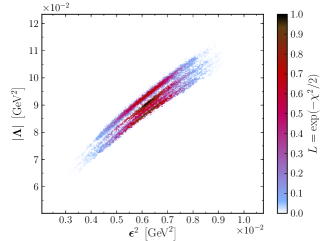
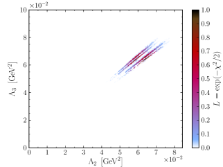
One general result of these and all following fits is that $\chi^{2}(\bm{a})$ is symmetric under the transformations $\Lambda_{i}\rightarrow-\Lambda_{i}$ and $\epsilon_{i}\to-\epsilon_{i}$, i. e. for a given minimum there are several other minima with the same goodness of fit which only differ in the signs of the $R$-parity breaking parameters. Independent of the specific mSUGRA point, the $\chi^{2}$-landscape of these fits is rather complex with 8 minima per sign combination of the $\Lambda_{i}$, resulting in 64 minima in total and each of them having $\chi^{2}$-values of less than $10^{-5}$. For a specific choice of signs for the $\Lambda_{i}$, the 8 minima divide into two classes of 4 minima each which differ by the importance of their individual loop contributions. These minima can be differentiated by the sign of the ratio $\epsilon_{2}\epsilon_{3}/(\Lambda_{2}\Lambda_{3})$ Hirsch et al. (2000); Diaz et al. (2003a). For $\epsilon_{2}\epsilon_{3}/(\Lambda_{2}\Lambda_{3})<0$, which is realized in the lower two plots of Figure 1 for $\Lambda_{3}\raise 1.29167pt\hbox{$\;<$\kern-7.5pt\raise-4.73611pt\hbox{$\sim\;$}}0.05$ GeV², the most important contributions to the solar masses and mixings come from bottom/sbottom and chargino/charged-scalar loops, while for minima where $\epsilon_{2}\epsilon_{3}/(\Lambda_{2}\Lambda_{3})>0$ (regions with $\Lambda_{3}\raise 1.29167pt\hbox{$\;>$\kern-7.5pt\raise-4.73611pt\hbox{$\sim\;$}}0.05$ GeV²) the corrections from bottom/sbottom loops are dominant. In the latter case also eqs. (7) get sizable corrections, in particular $\tan^{2}\theta_{13}$. This can also be inferred from the right upper plot of Figure 1. In the region in the upper left corner the atmospheric neutrino mass scale are essentially given by the tree level whereas in the lower two regions sizeable loop corrections are needed. The ratio $\bm{\epsilon}^{2}/|\bm{\Lambda}|$ gives the importance of the loop contributions relative to the tree-level-induced neutrino masses Hirsch et al. (2000). In the left upper plot we show preferred regions in the $\epsilon_{2}$-$\epsilon_{3}$ plane to demonstrate the sign ambiguities of the underlying parameters. Note, that in the lower two plots only one quadrant is shown and the remaining ones can be obtained by mirroring similar to the upper left.

The absolute uncertainties on these parameters depend clearly on the $R$-parity conserving parameters but the relative uncertainties are fairly insensitive to the $R$-parity conserving parameters. However, up to now we have ignored their uncertainties as we only took neutrino data into account. In the next sections we will add collider observables to allow also for a variation of these parameters.

IV.3 Neutralino decay properties

We now investigate how the neutralino decay properties can be used to get information on the $R$-parity breaking parameters without using neutrino data. We will use the $\tilde{\chi}^{0}_{1}$ decay width and branching ratios as data points for the fits but keep the other collider observables fixed. Of the branching ratios only those were taken into account whose values exceeded $0.01\text{\,}\%$. The relative uncertainties of the branching ratios were assumed to be $\Delta\mathrm{BR}_{i}/\mathrm{BR}_{i}=2/\sqrt{N_{i}}$ with $N_{i}=2\cdot 10^{6}\ \mathrm{BR}_{i}$ for a LHC integrated luminosity of $100\text{\,}\mathrm{f}\mathrm{b}^{-1}$ Aguilar-Saavedra et al. (2006). In the uncertainties of branching ratios whose final state contained quarks or $\tau$ leptons we reduced the corresponding number $N_{i}$ to $N_{i}/10$ in order to take potential uncertainties in the jet reconstruction into account. In principle this has to be checked by detailed Monte Carlo studies which are however beyond the scope of this article.

Figure 2: Likelihood map of the $\epsilon_{2}\Lambda_{2}$-$\epsilon_{3}\Lambda_{3}$ plain of fits at SPS 1a^′ with the $\tilde{\chi}^{0}_{1}$ decay properties (compare subsection IV.3). The plot shows that the distinct regions which correspond to different sets of open decay channels have different signs for $\epsilon_{2}\Lambda_{2}$ and $\epsilon_{3}\Lambda_{3}$ and that for the global minimum $\epsilon_{2}\Lambda_{2}<0$ and $\epsilon_{3}\Lambda_{3}>0$. A fit with the neutrino and neutralino data combined will therefore favor points with this sign combinations.

Figure 3: Likelihood maps of fits at SPS 1a^′ for various parameter combinations using neutralino decay width and neutralino branching ratios: $\epsilon_{1}$-$\epsilon_{2}$ (upper left), $\bm{\epsilon}^{2}$-$|\bm{\Lambda}|$ (upper right), $\Lambda_{1}$-$\Lambda_{3}$ (lower left) and $\Lambda_{2}$-$\Lambda_{3}$ (lower right). In the lower two only one quadrant is shown, the others can be obtained by mirroring with respect to the axes. These maps are projections of the six-dimensional parameter space onto the corresponding planes such that points with a higher likelihood cover points with a lower likelihood. The regions with maximum likelihood (black) correspond to minimal $\chi^{2}$-values. See section IV.3 for further details.

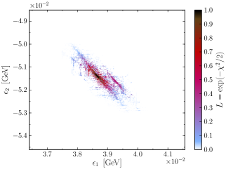
As already mentioned in subsection IV.2, the $\chi^{2}(\bm{a})$ of this fit is also symmetric under sign transformations of the $\Lambda_{i}$, i. e. also the decay properties of the $\tilde{\chi}^{0}_{1}$ do not depend on the sign of the alignment parameters. However, as can be seen in Figure 2 looking at the parameter combinations $\epsilon_{2}\Lambda_{2}$ and $\epsilon_{3}\Lambda_{3}$ one can identify a preferred quadrant, in this case the upper left, where all points with likelihood larger than 0.9 are located.

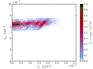
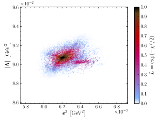
Compared to the previous fits, the regions with a high goodness of fit is reduced which is partly due to the higher number of degrees of freedom of this fit (13 data points and 6 free parameters). There are now also distinct regions with a high goodness of fit (each with its own local minimum) that correspond to different sets of decay channels whose branching ratio exceeds the aforementioned threshold of $0.01\text{\,}\%$. These regions can be seen in the two right plots of Figure 3. Within this setup the most important observables for the determination of the $R$-parity breaking parameters can be inferred by counting the frequency of those observables with the highest $\chi^{2}$-contributions for different minima. For SPS 1a^′ one finds for minima with $\chi^{2}<1$ that the four branching ratios with the highest $\chi^{2}$-contributions are

$$\mathrm{BR}(\tilde{\chi}^{0}_{1}\to\tau\tau\nu)\,,\quad\mathrm{BR}(\tilde{\chi}^{0}_{1}\to\tau\mu\nu)\,,\quad\mathrm{BR}(\tilde{\chi}^{0}_{1}\to\mu\mu\nu)\,,\quad\mathrm{BR}(\tilde{\chi}^{0}_{1}\to b\overline{b}\nu)\,.$$ (11)

Note, that this finding depends to some extent on the parameter point under study, e. g. for SPS 1b the most important branching ratios are

$$\mathrm{BR}(\tilde{\chi}^{0}_{1}\to\tau\mu\nu)\,,\quad\mathrm{BR}(\tilde{\chi}^{0}_{1}\to\tau e\nu)\,,\quad\mathrm{BR}(\tilde{\chi}^{0}_{1}\to S^{0}_{1}\nu)\,,\quad\mathrm{BR}(\tilde{\chi}^{0}_{1}\to b\overline{b}\nu)\,,$$ (12)

whereas for SPS 3 they are

$$\mathrm{BR}(\tilde{\chi}^{0}_{1}\to\tau e\nu)\,,\quad\mathrm{BR}(\tilde{\chi}^{0}_{1}\to\mu\mu\nu)\,,\quad\mathrm{BR}(\tilde{\chi}^{0}_{1}\to\tau\mu\nu)\,,\quad\mathrm{BR}(\tilde{\chi}^{0}_{1}\to b\overline{b}\nu)\,.$$ (13)

Moreover, it is obvious by comparing Figures 1 and 3 that neutrino data and branching ratios give complementary information.

IV.4 Combination of neutrino and neutralino data

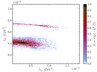
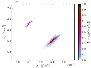
In this section we are combining the previous two fits and add also other observables: the $R$-parity breaking parameters are now fitted to the neutrino oscillation data and to the $\tilde{\chi}^{0}_{1}$ decay properties. Due to the combination of the data points, the regions with a high goodness of fit is significantly reduced as can be seen in Figure 4. Note, the different scaling of the axes compared to the previous plots. For SPS 1a^′ the parameter point $\widehat{\bm{a}}$ and all of its reflections with respect to the $\Lambda_{i}$ axes are now the only minima with $\chi^{2}\simeq 0$. For these points $\epsilon_{2}\Lambda_{2}<0$ and $\epsilon_{3}\Lambda_{3}>0$ hold. In the range $\chi^{2}<10$ there is only one additional minimum with $\chi^{2}\approx 1.5$ and for which $\epsilon_{2}\Lambda_{2}>0$ and $\epsilon_{3}\Lambda_{3}<0$.

Figure 4: Likelihood maps of fits at SPS 1a^′ for various parameter combinations using neutralino decay width and neutralino branching ratios: $\epsilon_{1}$-$\epsilon_{2}$ (upper left), $\bm{\epsilon}^{2}$-$|\bm{\Lambda}|$ (upper right), $\Lambda_{1}$-$\Lambda_{3}$ (lower left) and $\Lambda_{2}$-$\Lambda_{3}$ (lower right). In all but the upper right only one quadrant is shown, the others can be obtained by mirroring with respect to the axes. These maps are projections of the six-dimensional parameter space onto the corresponding planes such that points with a higher likelihood cover points with a lower likelihood. The regions with maximum likelihood (black) correspond to minimal $\chi^{2}$-values. See section IV.4 for further details.

SPS 1a′
parameter	best fit	$2\sigma$	$3\sigma$
$\epsilon_{1}\ \left[$10^{-2}\text{\,}\mathrm{G}\mathrm{e}\mathrm{V}$\right]$	$3.87\pm 0.03$	$\pm 0.07$	${}^{+0.11}_{-0.10}$
$\epsilon_{2}\ \left[$10^{-2}\text{\,}\mathrm{G}\mathrm{e}\mathrm{V}$\right]$	$-5.14\pm 0.04$	$\pm 0.09$	$\pm 0.13$
$\epsilon_{3}\ \left[$10^{-2}\text{\,}\mathrm{G}\mathrm{e}\mathrm{V}$\right]$	$4.55^{+0.10}_{-0.08}$	${}^{+0.22}_{-0.19}$	${}^{+0.32}_{-0.29}$
$\Lambda_{1}\ \left[$10^{-1}\text{\,}\mathrm{G}\mathrm{e}\mathrm{V}$^{2}\right]$	$0.03^{+0.04}_{-0.10}$	${}^{+0.08}_{-0.13}$	${}^{+0.11}_{-0.16}$
$\Lambda_{2}\ \left[$10^{-2}\text{\,}\mathrm{G}\mathrm{e}\mathrm{V}$^{2}\right]$	$6.41^{+0.05}_{-0.04}$	${}^{+0.11}_{-0.10}$	${}^{+0.16}_{-0.15}$
$\Lambda_{3}\ \left[$10^{-2}\text{\,}\mathrm{G}\mathrm{e}\mathrm{V}$^{2}\right]$	$6.41\pm 0.05$	${}^{+0.12}_{-0.13}$	$\pm 0.18$

SPS 3
parameter	best fit	$2\sigma$	$3\sigma$
$\epsilon_{1}\ \left[$10^{-2}\text{\,}\mathrm{G}\mathrm{e}\mathrm{V}$\right]$	$6.88\pm 0.04$	${}^{+0.15}_{-0.14}$	$\pm 0.18$
$\epsilon_{2}\ \left[$10^{-2}\text{\,}\mathrm{G}\mathrm{e}\mathrm{V}$\right]$	$-9.14\pm 0.05$	$\pm 0.17$	$\pm 0.22$
$\epsilon_{3}\ \left[$10^{-2}\text{\,}\mathrm{G}\mathrm{e}\mathrm{V}$\right]$	$8.09\pm 0.10$	$\pm 0.33$	${}^{+0.42}_{-0.43}$
$\Lambda_{1}\ \left[$10^{-1}\text{\,}\mathrm{G}\mathrm{e}\mathrm{V}$^{2}\right]$	$0.05^{+0.02}_{-0.11}$	${}^{+0.05}_{-0.15}$	${}^{+0.06}_{-0.17}$
$\Lambda_{2}\ \left[$10^{-2}\text{\,}\mathrm{G}\mathrm{e}\mathrm{V}$^{2}\right]$	$10.84\pm 0.06$	$\pm 0.19$	$\pm 0.24$
$\Lambda_{3}\ \left[$10^{-2}\text{\,}\mathrm{G}\mathrm{e}\mathrm{V}$^{2}\right]$	$10.84\pm 0.06$	$\pm 0.21$	${}^{+0.26}_{-0.27}$

Table 1: Parameter point $\widehat{\bm{a}}$ at SPS 1a^′ and SPS 3 with $1\sigma$, $2\sigma$, and $3\sigma$ uncertainties (12 d. f.) from fits with the neutrino oscillation data and the $\tilde{\chi}^{0}_{1}$ decay properties.

SPS 1a′
parameter	best fit	$2\sigma$	$3\sigma$
$\epsilon_{1}\ \left[$10^{-2}\text{\,}\mathrm{G}\mathrm{e}\mathrm{V}$\right]$	$3.87\pm 0.03$	${}^{+0.08}_{-0.07}$	${}^{+0.12}_{-0.11}$
$\epsilon_{2}\ \left[$10^{-2}\text{\,}\mathrm{G}\mathrm{e}\mathrm{V}$\right]$	$-5.14\pm 0.04$	$\pm 0.09$	$\pm 0.15$
$\epsilon_{3}\ \left[$10^{-2}\text{\,}\mathrm{G}\mathrm{e}\mathrm{V}$\right]$	$4.55^{+0.10}_{-0.08}$	${}^{+0.22}_{-0.19}$	${}^{+0.33}_{-0.30}$
$\Lambda_{1}\ \left[$10^{-1}\text{\,}\mathrm{G}\mathrm{e}\mathrm{V}$^{2}\right]$	$0.03^{+0.04}_{-0.09}$	${}^{+0.07}_{-0.14}$	${}^{+0.10}_{-0.16}$
$\Lambda_{2}\ \left[$10^{-2}\text{\,}\mathrm{G}\mathrm{e}\mathrm{V}$^{2}\right]$	$6.41\pm 0.04$	$\pm 0.10$	$\pm 0.16$
$\Lambda_{3}\ \left[$10^{-2}\text{\,}\mathrm{G}\mathrm{e}\mathrm{V}$^{2}\right]$	$6.41\pm 0.05$	$\pm 0.12$	${}^{+0.17}_{-0.18}$

SPS 3
parameter	best fit	$2\sigma$	$3\sigma$
$\epsilon_{1}\ \left[$10^{-2}\text{\,}\mathrm{G}\mathrm{e}\mathrm{V}$\right]$	$6.88\pm 0.05$	$\pm 0.12$	$\pm 0.20$
$\epsilon_{2}\ \left[$10^{-2}\text{\,}\mathrm{G}\mathrm{e}\mathrm{V}$\right]$	$-9.14\pm 0.06$	$\pm 0.15$	$\pm 0.25$
$\epsilon_{3}\ \left[$10^{-2}\text{\,}\mathrm{G}\mathrm{e}\mathrm{V}$\right]$	$8.09\pm 0.11$	$\pm 0.26$	${}^{+0.42}_{-0.43}$
$\Lambda_{1}\ \left[$10^{-1}\text{\,}\mathrm{G}\mathrm{e}\mathrm{V}$^{2}\right]$	$0.05^{+0.02}_{-0.12}$	${}^{+0.06}_{-0.15}$	${}^{+0.09}_{-0.20}$
$\Lambda_{2}\ \left[$10^{-2}\text{\,}\mathrm{G}\mathrm{e}\mathrm{V}$^{2}\right]$	$10.84\pm 0.06$	$\pm 0.15$	${}^{+0.24}_{-0.25}$
$\Lambda_{3}\ \left[$10^{-2}\text{\,}\mathrm{G}\mathrm{e}\mathrm{V}$^{2}\right]$	$10.84^{+0.07}_{-0.06}$	${}^{+0.15}_{-0.17}$	${}^{+0.25}_{-0.26}$

Table 2: Parameter point $\widehat{\bm{a}}$ at SPS 1a^′ and SPS 3 with $1\sigma$, $2\sigma$, and $3\sigma$ uncertainties (30 d. f.) from fits with the “LHC” setup.

SPS 1a′
parameter	best fit	$2\sigma$	$3\sigma$
$\epsilon_{1}\ \left[$10^{-2}\text{\,}\mathrm{G}\mathrm{e}\mathrm{V}$\right]$	$3.87\pm 0.03$	${}^{+0.08}_{-0.07}$	$\pm 0.12$
$\epsilon_{2}\ \left[$10^{-2}\text{\,}\mathrm{G}\mathrm{e}\mathrm{V}$\right]$	$-5.14\pm 0.04$	$\pm 0.09$	$\pm 0.15$
$\epsilon_{3}\ \left[$10^{-2}\text{\,}\mathrm{G}\mathrm{e}\mathrm{V}$\right]$	$4.55^{+0.10}_{-0.08}$	${}^{+0.22}_{-0.19}$	${}^{+0.34}_{-0.31}$
$\Lambda_{1}\ \left[$10^{-1}\text{\,}\mathrm{G}\mathrm{e}\mathrm{V}$^{2}\right]$	$0.03^{+0.04}_{-0.09}$	${}^{+0.07}_{-0.13}$	${}^{+0.10}_{-0.16}$
$\Lambda_{2}\ \left[$10^{-2}\text{\,}\mathrm{G}\mathrm{e}\mathrm{V}$^{2}\right]$	$6.41^{+0.04}_{-0.05}$	$\pm 0.10$	${}^{+0.17}_{-0.16}$
$\Lambda_{3}\ \left[$10^{-2}\text{\,}\mathrm{G}\mathrm{e}\mathrm{V}$^{2}\right]$	$6.41\pm 0.05$	${}^{+0.10}_{-0.11}$	${}^{+0.18}_{-0.17}$

SPS 3
parameter	best fit	$2\sigma$	$3\sigma$
$\epsilon_{1}\ \left[$10^{-2}\text{\,}\mathrm{G}\mathrm{e}\mathrm{V}$\right]$	$6.88\pm 0.05$	$\pm 0.12$	$\pm 0.20$
$\epsilon_{2}\ \left[$10^{-2}\text{\,}\mathrm{G}\mathrm{e}\mathrm{V}$\right]$	$-9.14\pm 0.06$	$\pm 0.15$	${}^{+0.25}_{-0.24}$
$\epsilon_{3}\ \left[$10^{-2}\text{\,}\mathrm{G}\mathrm{e}\mathrm{V}$\right]$	$8.09\pm 0.11$	$\pm 0.26$	${}^{+0.42}_{-0.43}$
$\Lambda_{1}\ \left[$10^{-1}\text{\,}\mathrm{G}\mathrm{e}\mathrm{V}$^{2}\right]$	$0.05^{+0.02}_{-0.12}$	${}^{+0.05}_{-0.15}$	${}^{+0.09}_{-0.19}$
$\Lambda_{2}\ \left[$10^{-2}\text{\,}\mathrm{G}\mathrm{e}\mathrm{V}$^{2}\right]$	$10.84\pm 0.06$	$\pm 0.15$	${}^{+0.25}_{-0.24}$
$\Lambda_{3}\ \left[$10^{-2}\text{\,}\mathrm{G}\mathrm{e}\mathrm{V}$^{2}\right]$	$10.84^{+0.06}_{-0.07}$	${}^{+0.15}_{-0.16}$	${}^{+0.24}_{-0.26}$

Table 3: Parameter point $\widehat{\bm{a}}$ at SPS 1a^′ and SPS 3 with $1\sigma$, $2\sigma$, and $3\sigma$ uncertainties (46 d. f.) from fits with the “LHC+ILC” setup.

Tables 1-3 give the uncertainties of the $R$-parity breaking parameters inferred from these fits for the “neutrino+neutralino data”, the “LHC”, and the “LHC+ILC” setup for SPS 1a^′ and SPS 3. The main uncertainties are due to the uncertainties of the neutrino data and the neutralino decay branching ratios a s can bee seen by comparing Table 1 with Tables 2 and 3. Except from $\Lambda_{1}$ the percentage errors of the $R$-parity breaking parameters at the $3\sigma$-level is less than $8\text{\,}\%$. $\Lambda_{1}$ is particularly difficult as the corresponding branching ratio $\tilde{\chi}^{0}_{1}\to W^{\pm}e^{\mp}$ is very small leading to the large uncertainties obtained. Note, that within the top-down approach, this means fitting the high scale mSUGRA parameters, there is hardly an effect on the uncertainties of the RPV parameters when going from the LHC to ILC. However, we do not expect significant differences when a fit of the $R$-parity conserving parameters is performed at the electroweak scale provided the neutralino and chargino masses can be measured within $1-2\text{\,}\%$ which is feasible at the ILC Accomando et al. (1998); Weiglein et al. (2006) or at CLIC Alster and Battaglia (2011). For the masses of the staus, sbottoms and the corresponding mixing angle one would need an accuracy of $10-20\text{\,}\%$ percent to keep the corresponding uncertainties in the calculation of the neutrino masses and mixing angles small enough so that they are sub-dominant compared to the uncertainties due to the branching ratios uncertainties. An important question will of course be on how much better the neutralino branching ratios can be measured at the ILC or CLIC compared to LHC.

V Discussion and conclusions

In this paper we have investigated the question how well one can measure $R$-parity violating couplings using neutrino data and future collider data. For simplicity we have taken bilinear $R$-parity violating parameters and fixed the $R$-parity conserving ones by imposing mSUGRA boundary conditions. The latter choice is not important as the requirement of explaining correctly neutrino data only fixes ratios of $R$-parity violating parameters over $R$-parity conserving parameters.

For the fits we have taken the current experimental accuracies on neutrino data and the expected accuracies on the measurements of edge variables at the LHC and mass measurements at the ILC as given by the corresponding collider studies. In addition we have assumed that at the LHC the decay length of the lightest neutralino can be measured within 15 percent and that the branching ratios can be determined within twice the corresponding statistical uncertainties. Under this assumptions we find that the expected accuracies on the RPV parameters is of order one percent. However, all fits show that there will be a sign ambiguity as all observables considered are nearly the same under a sign change of the RPV parameters. This ambiguities might be resolved by detailed studies of the lepton and jet spectra of the individual decay channels of the lightest supersymmetric particle, in the case under study the lightest neutralino.

The main source of the uncertainties are due to the uncertainties on the neutralino branching ratios. This implies that in a top-down approach, e. g. fitting the $R$-parity conserving within a given high scale model such as mSUGRA, the main information is already obtained at the LHC even if the ILC measures the SUSY spectrum more precisely. However, improvements are expected if at at ILC the neutralino branching ratios can be measured significantly better than at the LHC as one would naively presume. In case one fits the $R$-parity conserving parameters at the electroweak scale, then our findings hold if the masses of neutralinos, charginos, staus and sbottoms as well as the corresponding mixing matrices can be determined precisely. To keep things at the level shown (up to about a factor 1.5 – 2) one needs in case of the neutralino and charginos sectors precision in the percent-range, in stau and sbottom sector $10\text{\,}\%$ accuracies implying the need of an ILC and most likely also a multi-TeV $e^{+}e^{-}$ collider such as CLIC.

References

- Nath et al. (2010) P. Nath et al., Nucl. Phys. Proc. Suppl. 200-202, 185 (2010), eprint 1001.2693.
- Hirsch and Valle (2004) M. Hirsch and J. W. F. Valle, New J. Phys. 6, 76 (2004), eprint hep-ph/0405015.
- Hall and Suzuki (1984) L. J. Hall and M. Suzuki, Nucl. Phys. B231, 419 (1984).
- Hempfling (1996) R. Hempfling, Nucl. Phys. B478, 3 (1996), eprint hep-ph/9511288.
- Nardi (1997) E. Nardi, Phys. Rev. D55, 5772 (1997), eprint hep-ph/9610540.
- Kaplan and Nelson (2000) D. E. Kaplan and A. E. Nelson, JHEP 01, 033 (2000), eprint hep-ph/9901254.
- Hirsch et al. (2000) M. Hirsch, M. A. Diaz, W. Porod, J. C. Romao, and J. W. F. Valle, Phys. Rev. D62, 113008 (2000), eprint hep-ph/0004115.
- Diaz et al. (2003a) M. A. Diaz, M. Hirsch, W. Porod, J. C. Romao, and J. W. F. Valle, Phys. Rev. D68, 013009 (2003a), eprint hep-ph/0302021.
- Santamaria and Valle (1987) A. Santamaria and J. W. F. Valle, Phys. Lett. B195, 423 (1987).
- Romao and Valle (1992) J. C. Romao and J. W. F. Valle, Nucl. Phys. B381, 87 (1992).
- Nilles and Polonsky (1997) H.-P. Nilles and N. Polonsky, Nucl. Phys. B484, 33 (1997), eprint hep-ph/9606388.
- Kitano and Oda (2000) R. Kitano and K.-y. Oda, Phys. Rev. D61, 113001 (2000), eprint hep-ph/9911327.
- Mukhopadhyaya et al. (1998) B. Mukhopadhyaya, S. Roy, and F. Vissani, Phys. Lett. B443, 191 (1998), eprint hep-ph/9808265.
- Porod et al. (2001) W. Porod, M. Hirsch, J. Romao, and J. W. F. Valle, Phys. Rev. D63, 115004 (2001), eprint hep-ph/0011248.
- Hirsch et al. (2002) M. Hirsch, W. Porod, J. C. Romao, and J. W. F. Valle, Phys. Rev. D66, 095006 (2002), eprint hep-ph/0207334.
- Hirsch and Porod (2003) M. Hirsch and W. Porod, Phys. Rev. D68, 115007 (2003), eprint hep-ph/0307364.
- Barger et al. (2002) V. D. Barger, T. Han, S. Hesselbach, and D. Marfatia, Phys. Lett. B538, 346 (2002), eprint hep-ph/0108261.
- Magro et al. (2003) M. B. Magro et al., JHEP 09, 071 (2003), eprint hep-ph/0304232.
- de Campos et al. (2005a) F. de Campos et al., Phys. Rev. D71, 075001 (2005a), eprint hep-ph/0501153.
- de Campos et al. (2008a) F. de Campos et al., JHEP 05, 048 (2008a), eprint 0712.2156.
- De Campos et al. (2010) F. De Campos, O. Eboli, M. Hirsch, M. Magro, W. Porod, et al., Phys.Rev. D82, 075002 (2010), eprint 1006.5075.
- Blair et al. (2001) G. A. Blair, W. Porod, and P. M. Zerwas, Phys. Rev. D63, 017703 (2001), eprint hep-ph/0007107.
- Blair et al. (2003) G. A. Blair, W. Porod, and P. M. Zerwas, Eur. Phys. J. C27, 263 (2003), eprint hep-ph/0210058.
- Bechtle et al. (2006) P. Bechtle, K. Desch, W. Porod, and P. Wienemann, Eur. Phys. J. C46, 533 (2006), eprint hep-ph/0511006.
- Lafaye et al. (2008) R. Lafaye, T. Plehn, M. Rauch, and D. Zerwas, Eur. Phys. J. C54, 617 (2008), eprint 0709.3985.
- Bechtle et al. (2010) P. Bechtle, K. Desch, M. Uhlenbrock, and P. Wienemann, Eur. Phys. J. C66, 215 (2010), eprint 0907.2589.
- Adam et al. (2011) C. Adam et al., Eur. Phys. J. C71, 1520 (2011), eprint 1007.2190.
- Hirsch et al. (2011) M. Hirsch, L. Reichert, and W. Porod (2011), eprint 1101.2140.
- Diaz et al. (1998) M. A. Diaz, J. C. Romao, and J. W. F. Valle, Nucl. Phys. B524, 23 (1998), eprint hep-ph/9706315.
- Dedes et al. (2006) A. Dedes, S. Rimmer, and J. Rosiek, JHEP 08, 005 (2006), eprint hep-ph/0603225.
- Hirsch et al. (2005) M. Hirsch, W. Porod, and D. Restrepo, JHEP 03, 062 (2005), eprint hep-ph/0503059.
- Hirsch and Valle (1999) M. Hirsch and J. W. F. Valle, Nucl. Phys. B557, 60 (1999), eprint hep-ph/9812463.
- Diaz et al. (2003b) M. A. Diaz, R. A. Lineros, and M. A. Rivera, Phys. Rev. D67, 115004 (2003b), eprint hep-ph/0210182.
- de Campos et al. (2005b) F. de Campos et al., Phys. Rev. D71, 055008 (2005b), eprint hep-ph/0409043.
- de Campos et al. (2008b) F. de Campos et al., Phys. Rev. D77, 115025 (2008b), eprint 0803.4405.
- Porod (2003) W. Porod, Comput. Phys. Commun. 153, 275 (2003), eprint hep-ph/0301101.
- Schwetz et al. (2008) T. Schwetz, M. A. Tortola, and J. W. F. Valle, New J. Phys. 10, 113011 (2008), eprint 0808.2016.
- James and Roos (1975) F. James and M. Roos, Comput. Phys. Commun. 10, 343 (1975).
- Allanach et al. (2009) B. Allanach et al., Comp. Phys. Commun. 180, 8 (2009), eprint 0801.0045.
- Skands et al. (2004) P. Skands et al., JHEP 07, 036 (2004), eprint hep-ph/0311123.
- Weiglein et al. (2006) G. Weiglein et al. (LHC/LC Study Group), Phys. Rept. 426, 47 (2006), eprint hep-ph/0410364.
- Aguilar-Saavedra et al. (2006) J. A. Aguilar-Saavedra et al., Eur. Phys. J. C46, 43 (2006), eprint hep-ph/0511344.
- Allanach et al. (2002) B. C. Allanach et al., Eur. Phys. J. C25, 113 (2002), eprint hep-ph/0202233.
- (44) F. Thomas, http://physik.uni-wuerzburg.de/~fthomas/brpv_fit/.
- Khachatryan et al. (2011) V. Khachatryan et al. (CMS), Phys. Lett. B698, 196 (2011), eprint 1101.1628.
- Aad et al. (2011) G. Aad et al. (Atlas) (2011), eprint 1102.2357.
- (47) E. Ros, private communication.
- Accomando et al. (1998) E. Accomando et al. (ECFA/DESY LC Physics Working Group), Phys. Rept. 299, 1 (1998), eprint hep-ph/9705442.
- Alster and Battaglia (2011) N. Alster and M. Battaglia (2011), eprint 1104.0523.