Turbulent Clustering of Protoplanetary Dust and Planetesimal Formation

Abstract

We study the clustering of inertial particles in turbulent flows and discuss its applications to dust particles in protoplanetary disks. Using numerical simulations, we compute the radial distribution function (RDF), which measures the probability of finding particle pairs at given distances, and the probability density function of the particle concentration. The clustering statistics depend on the Stokes number, $St$, defined as the ratio of the particle friction timescale, $\tau_{\rm p}$, to the Kolmogorov timescale in the flow. In agreement with previous studies, we find that, in the dissipation range, the clustering intensity strongly peaks at $St\simeq 1$, and the RDF for $St\sim 1$ shows a fast power-law increase toward small scales, suggesting that turbulent clustering may considerably enhance the particle collision rate. Clustering at inertial-range scales is of particular interest to the problem of planetesimal formation. At these large scales, the strongest clustering is from particles with $\tau_{\rm p}$ in the inertial range. Clustering of these particles occurs primarily around a scale where the eddy turnover time is $\sim\tau_{\rm p}$. We find that particles of different sizes tend to cluster at different locations, leading to flat RDFs between different particles at small scales. In the presence of multiple particle sizes, the overall clustering strength decreases as the particle size distribution broadens. We discuss particle clustering in two recent models for planetesimal formation. We point out that, in the model based on turbulent clustering of chondrule-size particles, the probability of finding strong clusters that can seed planetesimals may have been significantly overestimated. We discuss various clustering mechanisms in simulations of planetesimal formation by gravitational collapse of dense clumps of meter-size particles, in particular the contribution from turbulent clustering due to the limited numerical resolution.

1. Introduction

Dust grains with microscopic to millimeter size are an important component of many astrophysical environments, and perhaps most significantly of protoplanetary disks. Although they contain a small mass fraction (approximately 1% with no gas-grain separation), solid particles affect the gas dynamics and emission through various processes such as thermal exchange, surface chemistry, and radiative transfer. In protoplanetary disks, their migration, sedimentation, and collisional coalescence and fragmentation set the stage for planet formation. Solid particles are dragged by gas motions, which are generally turbulent in astrophysical systems. The drag force of the gas turbulence, along with the generic feature that the inertial particle trajectories are dissipative, gives these particles a complex dynamics consisting of stochastic accelerations and decelerations, resulting in motions that partially reflect features of the velocity field of the gas that carries them.

The effect of turbulence on particle or droplet growth has been studied for over half a century (Arenberg 1939, East &Marshall 1954), and remains a challenging problem today in many research fields, particularly in the study of turbulent atmospheres. It is relevant to cloud formation, rain initiation (see Shaw (2003) for a general review), and the general microphysics (Pruppacher and Klett 1998) of the atmospheres of planets and moons ( e.g. Barth and Rafkin 2007, McGouldrick and Toon 2008), and of cool stars and brown dwarfs (Helling and Woitke 2006, Helling et al. 2008, Marley, Didier, and Goldblatt 2010, Freytag et al. 2010).

For disks, an important effect is that turbulent motions can induce random relative velocities between inertial particles that are much larger than Brownian velocities, increasing the particle collision rates, and hence growth rates, but also leading to destructive collisions if the relative particle speed exceeds a threshold believed to be of order a few cm/sec (see Blum and Wurm (2008) for a review; Guttler et al. (2010) for an update). In the present paper we focus on another aspect of the coupling of turbulence with solid particles in disks: Turbulent clustering. Because the inertia of particles prevents a perfect coupling with the flow, dissipative trajectories forced by turbulence can cause the formation of dense clusters of particles, even if the flow is incompressible. The process is sometimes referred to as “preferential concentration” (Fessler et al. 1994) in atmospheric and engineering applications.

The ability of incompressible turbulence to generate clusters of small particles was suggested in a seminal paper by Maxey (1987), and has been confirmed both numerically (Squires & Eaton 1991; Wang & Maxey 1993) and experimentally (Fessler et al. 1994, Uhlig et al. 1998, Kostinski & Shaw 2001, Aliseda et al. 2002, Pinsky & Khain 2003, Wood et al. 2005, Lehmann et al. 2007). The basic features of turbulent clustering were established in a number of theoretical studies (Elperin et al. 1998a, Elperin et al. 1998b, Balkovsky et al. 2001, Zaichik et al. 2003a, Zaichik et al. 2003b, Elperin et al. 2002) and low-resolution simulations (Sundaram & Collins97, Zhou et al. 1998, Reade & Collins 2000a, Reade & Collins 2000b, Wang et al. 2000). Most of these studies focused on clustering at the dissipation-range scales. In this scale range, the clustering intensity was found to peak for particles with Stokes number (the ratio of particle friction time to the Kolmogorov timescale) close to unity, and the clustering amplitude was shown to increase towards smaller scales as a power law. Higher-resolution turbulence simulations (Hogan et al. 1999, Hogan& Cuzzi 2001, Collins & Keswani 2004, Falkovich & Pumir 2004, Bec et al. 2006a, Cencini et al. 2006) have confirmed these basic results, but still differ concerning the scaling of the clustering amplitude with the Stokes and Reynolds numbers.

The process of turbulent clustering has been proposed as a possible solution to the problem of raindrop formation in atmospheric clouds (Jameson& Kostinski 2000, Falkovich et al. 2002, Vaillancourt et al. 2002), due to its effects on the collision rate of droplets. As in the case of droplet formation, the collision rate between dust grains in astrophysical systems may be enhanced by turbulent clustering. A major goal of this paper is a general introduction of the phenomenon of turbulent clustering to the astronomy community, presenting a detailed physical discussion and numerical results. We also discuss the application of our simulation results to models of planetesimal formation in protoplanetary disks.

Planetesimals are kilometer-size objects believed to be the necessary precursors to the formation of fully-fledged rocky planets. The classic theory assumes that planetesimals form by gravitational instability, as the dust particles vertically settle to a dense thin layer at the midplane (Safronov 1969, Goldreich and Ward 1973). However, even without preexisting turbulence, size-differentiated sedimentation of the particles results in vertical shear that can lead to Kelvin-Helmholtz instabilities as suggested by Weidenschilling (1980) (see Barranco 2009 for a recent detailed study). The resulting turbulent mixing prevents the settling to a thin dust layer, and the dust density needed for the gravitational instability to occur may be difficult to achieve (e.g. Youdin and Shu 2002, Chiang 2008). Another possibility is that planetesimals form by the collisional growth of dust particles. Early work on collisional growth of planetesimals and planets was reviewed by Lissauer (1993). The most serious problem for planetesimal formation in a turbulent disk continues to be that both theoretical (e.g. Ormel et al. 2007, Brauer et al. 2008) and experimental (see Blum and Wurm 2008 for a thorough review) studies indicate that particle growth is stalled in the cm-m size range, a conundrum usually referred to as the meter-size problem. Fast radial migration of cm-m particles could be alleviated with a modest enhancement of the dust-to-gas ratio, but these particles acquire such large velocities that collisional fragmentation appears inevitable (see Brauer et al. 2008). A recent summary of work on planetesimal growth is presented by Chiang and Youdin (2010), who emphasize the possibility that drag instabilities can concentrate particles and initiate gravitational instability of particle clusters (Goodman and Pindor 2000, Youdin and Goodman 2005, Johansen et al. 2007).

One response to these problems is to use them to argue that turbulence must not exist. Another is to accept one of several mechanisms (see Chiang and Youdin 2010) suggested to avoid the meter-size problem. Some of these mechanisms are based on the formation of dense particle clumps by the clustering of particles by the disk turbulence (Cuzzi et al. 2008), or by the streaming instability and other clustering effects (Johansen et al. 2007, 2009a, 2011). The point of view of the present paper is to take a critical look at the aspects of the models that rely on clustering of small particles as a part of planetesimal formation, using a new high-resolution turbulence simulation, along with a set of approximate guidelines to the behavior we find.

The paper is organized as follows. §2 is a general introduction to the physics of turbulent clustering. In §3 we describe our numerical simulations. We present results on the clustering statistics of identical particles in §4. In this section, we also discuss the Reynolds number dependence and possible effects of the back reaction, largely based on a review of numerical results from the literature. The clustering statistics of particles of different sizes are presented in §5. We apply our understanding of turbulent clustering to the problem of planetesimal formation in §6, with specific discussions of the models by Cuzzi et al. (2008) and Johansen et al. (2007). Our conclusions are summarized in §7.

2. Inertial Particle Clustering in Turbulent Flows

In order to guide the interpretation of the numerical results, we present here a brief introduction to the problem of particle clustering. We show how simple physical arguments allow us to make rough predictions about the Stokes number dependence of turbulent clustering that will be computed later from our numerical simulation.

The velocity, $\boldsymbol{v}(t)$, of an inertial particle suspended in a turbulent velocity field, $\boldsymbol{u}(\boldsymbol{x},t)$, is given by the equation,

$$\frac{d\boldsymbol{v}}{dt}=\frac{\boldsymbol{u}(\boldsymbol{x}_{\rm p}(t),t)-\boldsymbol{v}}{\tau_{\rm p}}$$ (1)

where $\boldsymbol{u}(\boldsymbol{x}_{\rm p}(t),t)$ is the flow velocity along the particle trajectory, $\boldsymbol{x}_{\rm p}(t)$, and the friction timescale, $\tau_{\rm p}$, represents the particle inertia and is essentially the time needed for the particle velocity to relax toward the flow velocity through the friction force.

The estimate of the friction timescale depends on the particle size, $a_{\rm p}$, relative to the mean free path of the gas molecules, $\lambda_{\rm g}$, in the flow (see, e.g., Weidenschilling 1977; Cuzzi et al. 1993). If $a_{\rm p}\ll\lambda_{\rm g}$, the particle-flow friction is in the Epstein Regime where the drag force is controlled by collisions between the particle and the flow molecules. The friction time is calculated by,

$$\tau_{\rm p}=\left(\frac{\rho_{\rm d}}{\rho_{\rm g}}\right)\left(\frac{a_{\rm p}}{C_{\rm s}}\right)$$ (2)

where $C_{\rm s}$ is the gas thermal velocity, $\rho_{\rm g}$ is the density of the flow and $\rho_{\rm d}$ is the density of the particle material. For compact dust grains, $\rho_{\rm d}\sim 1$ g cm^-3. The gas mean free path is estimated by $1(\rho_{\rm g}/10^{-9}$ g cm^-3)^-1 cm, assuming the cross section of hydrogen molecules is $\sim 10^{-15}$ cm². Therefore, the friction between dust particles and the flow is in the Epstein regime for particle size up to $\sim 1(\rho_{\rm g}/10^{-9}$ g cm^-3)^-1 cm. Due to the density dependence, this critical size varies with the radial locations in the disk and depends on the disk parameters.

On the other hand, for particles with $a_{\rm p}\gg\lambda_{\rm g}$, the friction force is determined by the flow around the particle surface. If the flow around the particle is laminar, the friction timescale is given by the Stokes law,

$$\tau_{\rm p}=\frac{2}{9}\left(\frac{\rho_{\rm d}}{\rho_{\rm g}}\right)\left(\frac{a_{\rm p}^{2}}{\nu}\right)$$ (3)

where $\nu$ is the kinematic viscosity of the carrier flow.

The Stokes number, $St$, defined as the ratio of the friction timescale to the Kolmogorov timescale, $\tau_{\eta}$, i.e., $St\equiv\tau_{\rm p}/\tau_{\eta}$, is commonly used to characterize the particle inertia. The Kolmogorov timescale is essentially the turnover time of the smallest eddies and is thus the smallest timescale in a turbulent flow. It is defined as $\tau_{\eta}=(\nu/\bar{\epsilon})^{1/2}$ where $\bar{\epsilon}$ is the average energy dissipation rate. In incompressible turbulence, we have $\bar{\epsilon}=\nu\langle{\bf\omega}^{2}\rangle$ with ${\bf\omega}$ being vorticity, and thus $\tau_{\eta}$ can be calculated as $\tau_{\eta}=\langle\omega^{2}\rangle^{-1/2}$. It can also be roughly estimated from the large-scale properties of the flow by $\tau_{\eta}\simeq(L/U)Re^{-1/2}$ where $L$, $U$ and $Re$ are, respectively, the outer length scale, the rms flow velocity and the Reynolds number. A crucial length scale in the clustering statistics of inertial particles is the Kolmogorov dissipation scale, $\eta$, which is given by $\eta\equiv(\nu^{3}/\bar{\epsilon})^{1/4}\simeq LRe^{-3/4}$. Numerical values for these quantities applicable to disks are given in §6.1.

The spatial clustering of inertial particles in turbulent flows has different behaviors for $St<1$ and $St>1$. We discuss the two Stokes number ranges separately.

2.1. Particles with $St<1$

The trajectories of small particles with $St\ll 1$ deviate from those of the fluid elements only slightly, and the particle phase can be approximately described as a fluid. The velocity field, $v_{i}(\boldsymbol{x},t)$, of the particle flow can be estimated from eq. (1). Assuming that the particle acceleration, $\frac{dv_{i}}{dt}$, can be approximated by the local flow acceleration, $\frac{du_{i}}{dt}$, we have $v_{i}(\boldsymbol{x},t)\simeq u_{i}(\boldsymbol{x},t)-\tau_{\rm p}\frac{du_{i}}{dt}(\boldsymbol{x},t)$. The assumption is justified for $St\ll 1$ particles because the friction timescale $\tau_{\rm p}$ is smaller than $\tau_{\eta}$, the smallest timescale in the flow. The approximation is essentially the Taylor expansion of eq. (1) to the first order of $St$.

With this approximation, one can estimate the divergence, $\partial_{i}v_{i}$, of the particle velocity field. If the carrier flow is incompressible, we have,

$$\partial_{i}v_{i}=-\tau_{\rm p}\partial_{i}u_{j}\partial_{j}u_{i},$$ (4)

where we used $\frac{du_{i}}{dt}=\frac{\partial u_{i}}{\partial t}+u_{j}\partial_{j}u_{i}$ and $\partial_{i}u_{i}=0$. Eq. (4) suggests that the particle flow has a finite compressibility even though the carrier flow is incompressible, and this would lead to spatial clustering of the particles. Intuitively, the physical origin for clustering is that the particles’ inertia causes them to lag behind or lead in front of the flow elements when the flow experiences an acceleration or deceleration.

The amplitude of the particle velocity divergence depends on the flow velocity gradient. On average, the velocity gradient in a turbulent flow is $\sim(\bar{\epsilon}/\nu)^{1/2}=1/\tau_{\eta}$ (e.g., Monin and Yaglom 1975), thus we have an estimate that $\partial_{i}v_{i}\simeq St/\tau_{\eta}$. In the limit of small Stokes numbers, the divergence increases with increasing $St$, and thus the degree of clustering is expected to increase with $St$.

The particle velocity divergence can be rewritten as $\tau_{\rm p}(\omega^{2}/2-s_{ij}s_{ij})$ where $s_{ij}=(\partial_{i}u_{j}+\partial_{j}u_{i})/2$ is the strain tensor (Maxey 1987). This suggests that vorticity tends to expel particles, while the strain would collect particles. Therefore dense particle clusters are expected to be found in the strain-dominated regions with low vorticity. This effect is illustrated in Appendix A where we use Burgers vortex tubes as a model for the small-scale structures in turbulent flows. The effect of vortices as centrifuges for inertial particles was first recognized by Maxey (1987), and has been subsequently studied in details with both numerical simulations (e.g., Wang and Maxey 1993) and experiments (e.g., Fessler et al. 1994).

Eq. (4) can also be written as $\partial_{i}v_{i}=\tau_{\rm p}\partial_{i}^{2}P/\rho_{\rm g}$. This means that the particle flow divergence is negative at local pressure maxima where $\partial_{i}^{2}P/\rho_{\rm g}<0$. Therefore, particle clustering in turbulent flows is sometimes interpreted as collection of particles at local pressure maxima.

The velocity gradient field in a turbulent flow has a correlation length scale of $\eta$, and thus the divergence of the particle flow is decorrelated at scales larger than $\eta$. Therefore the probability for the existence of coherent particle compressions or expansions at scales significantly larger than $\eta$ would be rare, suggesting that, at $St\;\hbox to0.0pt{\lower 2.5pt\hbox{$\sim$}\hss}\raise 1.5pt\hbox{$<$}\;1$, particle clustering would primarily occur below the Kolmogorov length scale. However, this does not mean that the particle clusters appear as spheres of size $\sim\eta$. Instead, they are found to be in the form of filaments or sheets of thickness $\sim\eta$.

Particle clusters are subject to disruption by the stretching of the carrier flow, which tends to disperse the clusters. The balance between the disruption and the compressibility in the particle flow determines the clustering intensity. At smaller scales, it takes longer time for stretching to disperse particle clusters to scales larger than $\eta$ where essentially no coherent compressions or expansions exist. Therefore a higher level of clustering is expected at smaller scales because clusters at these scales can experience coherent compressions for longer time (Falkovich and Pumir 2004).

It is interesting to note that the quadratic dependence of the particle flow divergence on the velocity gradients is similar to that of the energy dissipation rate $\epsilon({\boldsymbol{x}},t)=\frac{1}{2}\nu(\partial_{i}u_{j}+\partial_{j}u_{i})^{2}$. Therefore, like the dissipation rate, $\partial_{i}v_{i}$ would also display spatial fluctuations, which may give rise to a broad probability density function (PDF) for the particle concentration. Also, it is known that the PDF of the energy dissipation rate broadens with increasing Reynolds number (Frisch 1995). A similar Reynolds number dependence is likely to exist for the concentration PDF of particles with $St\;\hbox to0.0pt{\lower 2.5pt\hbox{$\sim$}\hss}\raise 1.5pt\hbox{$<$}\;1$.

2.2. Particles with $St>1$

With increasing inertia, the particle trajectories deviate more from those of the flow elements. A large particle has a long memory, and its current velocity has significant contribution from the memory of the flow velocity in the past. Therefore, the particle velocity cannot be simply estimated by the local carrier flow. The approximation, eq. (4), for the particle flow divergence breaks down for $St$ larger than 1.

In fact, nearby large particles with $St\gg 1$ do not move coherently, and at small scales the particle phase can no longer be viewed as a fluid. Intuitively, due to their large inertia, two large particles can keep a significant relative speed when approaching each other. Therefore the relative particle motions at small scales appear to be random. Bec et al. (2010) found that, for $St>1$, the velocity difference, $\delta v(St,l)$, of two particles at a separation $l$ is constant at small values of $l$, indicating that their relative motions are similar to the thermal motions of molecules in kinetic theory. Thus a fluid description for these particles would not be sufficient. The physical reason for a constant $\delta v(St,l)$ at small $l$ (for a given $St$) is that the relative velocity between nearby particles is dominated by their memory of the flow velocity difference they “saw” within a friction timescale in the past (Pan and Padoan 2010).

We consider the response behavior of $St>1$ particles to turbulent eddies of different sizes, which provides physical insights to the clustering properties of these particles. A length scale of particular interest is the size of turbulent eddies whose turnover timescale is equal to the particle friction timescale, $\tau_{\rm p}$. If $\tau_{\rm p}$ corresponds to an inertial-range timescale of the carrier flow, we have $l_{\tau_{\rm p}}\simeq\bar{\epsilon}^{1/2}\tau_{\rm p}^{3/2}$ (or equivalently $\simeq St^{3/2}\eta$) using the Kolmogorov scaling.

Particles can efficiently respond to eddies much larger than $l_{\tau_{\rm p}}$. At these scales, the particle motions are well coupled to the flow elements, and the particle velocity difference, $\delta v(St,l)$, essentially follows the flow velocity difference, $\delta u(l)$ (see Bec et al. 2010). Therefore, no strong particle clustering is expected at these large scales. Eddies much smaller than $l_{\tau_{\rm p}}$ do not efficiently affect the relative particle motions because the particle response time, $\tau_{\rm p}$, is much longer than the eddy turnover time. Thus, at scales below $l_{\tau_{\rm p}}$, the flow and the particle motions are decoupled, and the relative velocity between two particles is determined by their memory of the flow velocity difference at scales around $l_{\tau_{\rm p}}$, where the particle motions are partially coupled to the carrier flow. As discussed above, particles show random relative motions at these small scales, and thus no clustering would be found at $l\ll l_{\tau_{\rm p}}$ either. This means that significant clustering could occur only around the scale $\sim l_{\tau_{\rm p}}$. This physical picture also suggests that the particle phase has an effective mean free path of $l_{\tau_{\rm p}}$. A fluid description for particles may be valid at scales above $l_{\tau_{\rm p}}$.

For particles with $\tau_{\rm p}$ larger than the turnover time, $T_{\rm L}$, at the outer scale of the flow, all eddies evolve at a timescale smaller than $\tau_{\rm p}$, and $l_{\tau_{\rm p}}$ cannot be defined. Such particles do not closely follow the flow velocity at any scale. Motions of these particles are expected to be random at all scales, and the spatial distribution would be essentially homogeneous. We focus on inertial-range particles with $\tau_{\eta}\ll\tau_{\rm p}\ll T_{\rm L}$ in our discussions.

The clustering intensity for inertial-range particles is expected to decrease with increasing $St$. As discussed above, these particles cluster primarily at the length scale, $l_{\tau_{\rm p}}$, which increases with $St$. Therefore, clusters of larger particles are spatially more spread out, and, since no strong fluctuations exist below $l_{\tau_{\rm p}}$, the concentration level within the clusters would decrease with increasing $St$. In other words, smaller particles can form thinner clusters with higher density contrast and hence exhibit stronger clustering. The decrease of the clustering intensity with $St$ is illustrated by an intuitive example in Appendix A. The example shows that larger particles (with $St>1$) form clusters of larger sizes, and the particle concentration in the clusters becomes smaller with increasing $St$.

We estimate the compressibility in the particle collective motions around the scale $l_{\tau_{\rm p}}$, which is used in Appendix B for the derivation of the Brownian scale. Here the scale $l_{\tau_{\rm p}}$ is of special interest because the maximum flow velocity gradient that the particles can efficiently “feel” is that at $l_{\tau_{\rm p}}$. The gradient is approximately $\delta u(l_{\tau_{\rm p}})/l_{\tau_{\rm p}}$, which is $\propto\bar{\epsilon}^{1/3}l_{\tau_{\rm p}}^{-2/3}$ using the Kolmogorov scaling. The gradient decreases as $(\tau_{\rm p})^{-1}$ with $\tau_{\rm p}$, which also suggests weaker clustering for larger particles. The divergence of the particle motions around the scale $l_{\tau_{\rm p}}$ is calculated by the same method (eq. 4) as for the $St<1$ particles. This is justified because the friction time is smaller than the turnover time of eddies larger than $l_{\tau_{\rm p}}$. Inserting $\delta u(l_{\tau_{\rm p}})/l_{\tau_{\rm p}}$ for the velocity gradients in eq. (4) shows that the effective divergence is $\sim\tau_{\rm p}^{-1}=(St\tau_{\eta})^{-1}$. Therefore, for $St\;\hbox to0.0pt{\lower 2.5pt\hbox{$\sim$}\hss}\raise 1.5pt\hbox{$>$}\;1$, the particle collective motions are less compressible as $St$ increases.

We note that, unlike particles with $St<1$, the effective divergence estimated above for $St>1$ only depends on the particle friction time, but not on the flow properties in the inertial range. This is because clustering of these particles occurs at scales “selected” by the particle timescale. At the selected length scale, the turnover timescale is around $\tau_{\rm p}$, and the flow velocity gradient is $\sim\tau_{\rm p}^{-1}$. It is thus not surprising that the effective divergence is determined solely by the friction timescale. The possibility of clustering of large particles at an inertial-range scale $\sim l_{\tau_{\rm p}}$ has also been discussed in earlier studies (e.g., Eaton and Fessler 1994, Boffetta et al. 2004, Bec et al.  2007).

In summary, inertial particles suspended in a turbulent flow are expected to show inhomogeneous spatial distribution even if the carrier flow is incompressible. Inertial particles tend to be expelled from vortices and accumulate in high-stain regions. For small particles with $St\;\hbox to0.0pt{\lower 2.5pt\hbox{$\sim$}\hss}\raise 1.5pt\hbox{$<$}\;1$, clustering occurs primarily at scales below the Kolmogorov scale $\eta$, and the degree of clustering increases with increasing $St$. Large particles with $1\;\hbox to0.0pt{\lower 2.5pt\hbox{$\sim$}\hss}\raise 1.5pt\hbox{$<$}\;St\;\hbox to0.0pt{\lower 2.5pt\hbox{$\sim$}\hss}\raise 1.5pt\hbox{$<$}\;T_{\rm L}/\tau_{\eta}$ cluster around a scale, $l_{\tau_{\rm p}}$, which increases with $St$ as $\simeq St^{3/2}\eta$. The clustering intensity decreases with $St$ for $St\;\hbox to0.0pt{\lower 2.5pt\hbox{$\sim$}\hss}\raise 1.5pt\hbox{$>$}\;1$. Overall, the clustering intensity is expected to peak at $St\sim 1$.

2.3. Clustering of particles of different sizes

The discussion above is for particles of the same size, an idealized situation usually referred to as the monodisperse case. In realistic environments, the particle size is likely to have significant variations either due to an initial size distribution (from the formation process of the particles) or as a result of collisional coagulation or fragmentation. Therefore it is necessary to consider the clustering statistics for particle of different sizes.

Numerical simulations by Zhou et al. (2001) showed that particles with different sizes tend to cluster at different locations in the flow (see also Reade and Collins 2000b). This is also clearly illustrated by our example in Appendix A. A consequence of this effect is that the probability of finding nearby particles of a different size is smaller than that of finding identical particles, given equal number densities of the two particles. This has interesting effects on the collision kernel for particle coagulation models (Reade and Collins 2000b). It also has important implications on the overall spatial distribution of particle density/concentration when the particles have an extended size range. A detailed analysis of the clustering statistics for particles of different sizes will be given in §5.

3. Numerical Simulations

With the rough but physically-motivated arguments of §2 in hand, we now present and interpret the results of our numerical simulation. The simulation was carried out in a periodic box with $512^{3}$ grid points. The hydrodynamic equations with an isothermal equation of state were solved by the Enzo code (O Shea et al. 2004 and references therein), which uses a direct Eulerian formulation of the Piecewise Parabolic Method (PPM) (Colella and Woodward 1984). To drive the turbulent flow and maintain the kinetic energy at the desired level, we apply a large-scale solenoidal force with a fixed spatial pattern and a constant power in the range of wave numbers $1\leq k\leq 2$. The amplitude of the driving force is chosen such that the rms Mach number, $M_{\rm s}$, in the flow is $\simeq 1$ (the simulation setup is the same as Kritsuk et al. (2007), except for the lower Mach number and the solenoidal forcing adopted here). Unlike previous simulations devoted to exploring particle clustering in incompressible turbulence (e.g. Sundaram & Collins 1997; Reade & Collins 2000a; Hogan & Cuzzi 2001; Collins & Keswani 2004; Falkovich & Pumir 2004; Cencini et al. 2006), our simulated flow is compressible.

We chose to study turbulent clustering with a compressible flow because we aimed at exploring dust grain dynamics in various environments including highly compressible interstellar clouds. In the current work, we will focus on the application in proptoplantary disks where the turbulence is essentially incompressible. We expect from the following considerations that the clustering statistics in our simulated flow would be close to that in incompressible turbulence. First, at Mach number close to unity, the density fluctuations are weak, with the rms amplitude $\langle\delta\rho_{\rm g}^{2}\rangle^{1/2}/\bar{\rho}_{\rm g}$ at the level of $\sim$10 percent. Second, the velocity structures in a transonic flow are very close to those in incompressible flows (Porter et al. 2002; Padoan et al. 2004; Pan and Scannapieco 2011). In §4.1, we find that the clustering properties in our transonic flow are indeed in good agreement with the results from direct numerical simulations (DNS) for incompressible flows by Collins & Keswani (2004). This agreement validates the application of our results to protoplanetary disks.

One important quantity in our statistical analysis is the Kolmogorov length scale. This length scale is difficult to evaluate because our PPM simulations do not explicitly include the viscous term and the kinetic energy dissipation is through numerical diffusion. We compute $\eta$ using two methods. In the first method, we start with an estimate of the effective viscosity, $\nu_{\rm eff}$. We calculate $\nu_{\rm eff}$ from the equation $\bar{\epsilon}=\nu_{\rm eff}\langle\omega_{i}^{2}\rangle$, because solenoidal modes dominate the kinetic energy dissipation even in a transonic flow (Pan and Scannapieco 2010). The energy dissipation rate, $\bar{\epsilon}$, can be derived either from Kolmogorov’s 4/5 law (which also applies also to transonic flows; see Pan and Scannapieco 2010 and also Benzi et al. 2008), or from the relation, $\bar{\epsilon}=Du^{\prime 3}/L_{1}$, established by DNS, where $u^{\prime}$ and $L_{1}$ are the 1D velocity dispersion and the integral length scale, and the coefficient $D\simeq 0.4$ (Ishihara et al. 2009). The dissipation rate values derived from the two approaches are consistent with each other. The effective viscosity $\nu_{\rm eff}$ is then calculated from $\bar{\epsilon}$ and $\langle w^{2}\rangle$. With $\nu_{\rm eff}$, we find the effective Taylor Reynolds number in our simulated flow is $Re_{\lambda}=250$. We calculate the Kolmogorov length scale from $\eta=(\nu_{\rm eff}^{3}/\bar{\epsilon})^{1/4}$, which turns out to be 1/2 the resolution scale (Benzi et al. 2008). The Kolmogorov timescale is computed by $\langle w^{2}\rangle^{-1/2}$.

Figure 1.— Second order velocity structure function in our simulated flow (data points). The dashed line is the structure function for an incompressible flow with $Re_{\lambda}=300$, obtained from a bridging formula that connects the established scaling behaviors in different scale ranges (see text).

In the second method, we estimate $\eta$ by comparing the 2nd order velocity structure function, $S(r)=\langle(v_{i}(\boldsymbol{x}+\boldsymbol{r},t)-v_{i}(\boldsymbol{x},t))^{2}\rangle$, in our flow to that established for incompressible turbulence from theory, experiments and simulations. We adjust the Kolmogorov scale (or equivalently the effective viscosity) in our flow to obtain a best fit. Our result is shown Fig. 1, where the length scale and the structure function are normalized to the Kolmogorov scale, $\eta$, and velocity, $u_{\eta}$, respectively. The data points represent the structure function measured in our simulated flow. The Kolmogorov scale is set to be 0.4 times the computation cell size. With this value for $\eta$, we estimated the effective viscosity and the Taylor Reynolds number. The latter is $\sim 300$. The dashed line is the expected structure function in an incompressible turbulent flow with $Re_{\lambda}=300$. It is obtained from a bridging formula given in Zaichik et al. (2006), which connects the established scaling behaviors of the structure function in different scale ranges. Clearly, the data points are in good agreement with the dashed line. This agreement suggests that our simulations can be safely used for the study of turbulent clustering in weakly compressible turbulence such as that in protoplanetary disks. The best-fit value for the Kolmogorov scale, 0.4 cell size, is close to that derived from first method, suggesting our estimate of $\eta$ is reliable. Throughout the paper, we set $\eta$ to be 0.4 cell size and assume the Taylor Reynolds number is 300.

A strength of the PPM method is that it yields a quite broad inertial range already at the resolution of $512^{3}$. A clear Kolmogorov scaling is seen in Fig. 1 at scales from $\simeq 30\eta$ to $\simeq 300\eta$ in the velocity structure function. To our knowledge, turbulent clustering has not been studied in simulations that have a clear inertial range. The inertial-range velocity scaling was used in our physical discussion in §2.2. Our numerical results show that the clustering behaviors are different at scales below and above the Kolmogorov scale $\eta$. We will refer to the scales below $\eta$ as the dissipation range, and loosely call the scale range $l>\eta$ the inertial range, although the latter usually refers to the scales showing a Komolgorov scaling.

Because the Kolmogorov scale is below the resolution scale, one may be concerned with the reliability and accuracy of the measured statistics around or below $\eta$. Fortunately, we find that the velocity field at the unsolved scales may be reliably approximated by interpolation. This is because the velocity structure function is already smooth at the resolution scale, as seen from the $r^{2}$ scaling at the smallest scales in Fig. 1. This scaling means that the velocity difference is linear with $r$, and a linear interpolation (see below) may sufficiently reflect the subgrid velocity statistics. Therefore, our simulation can provide good clustering statistics at scales around or below $\eta$. This is again supported by the agreement of our results with those from DNS simulations (see §4.1).

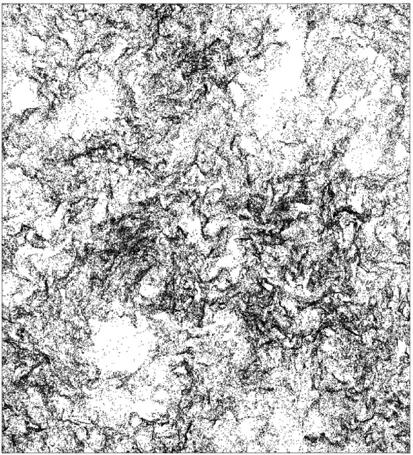
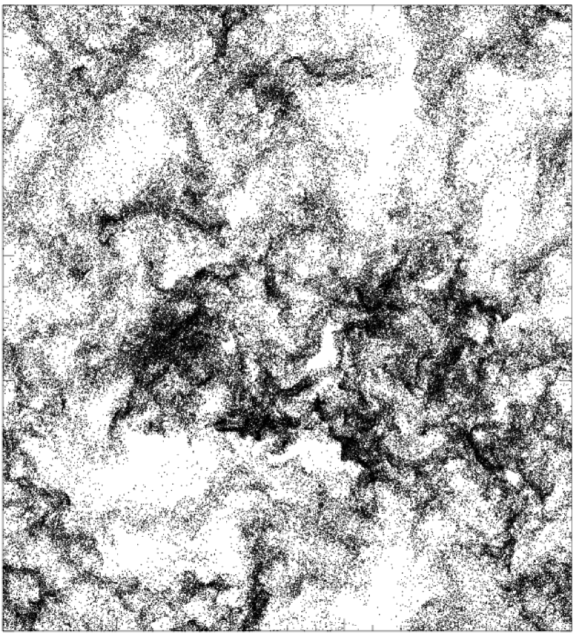
Figure 2.— Positions of all the particles with $St=1.2$ (left panel) and $St=4.9$ (right panel) within a thin slice of thickness equal to 2% of the computational box. Density fluctuations are much stronger for particles with $St=1.2$ than for those with $St=4.9$, but this cannot be fully appreciated from the images, due to the overlap of particle positions. Notice the very small scale structures present in the spatial distribution of the $St=1.2$ particles. Dense particle filaments and large voids can be seen in both panels, with sizes approaching the integral length of the flow, estimated to be approximately 0.2 times the computational box size. The estimated size of the dissipation scale, $\eta$, is approximately $10^{-3}$ times the box size, as discussed in §3.

We chose 16 different values for the particle size, and for each size we evolved 8.4 million particles in the simulated flow. The average particle density for each size is one per 16 computation cells. Due to the slight density fluctuations in our transonic flow, the friction timescale for a particle of a given size is not constant along its trajectory. The friction time scales with the gas density, $\rho_{\rm g}$, as $\tau_{\rm p}\propto\rho_{\rm g}^{-1}$ in the Epstein regime (the regime of primary interest in our astrophysical applications), and we calculated the local values of $\tau_{\rm p}$ using this scaling at each integration step for the particle trajectory. A linear interpolation is used to obtain the flow velocity and density at the particle positions inside the computation cells. A higher-order interpolation scheme may be needed for more accurate measurements of the clustering statistics below the resolution scale (e.g., Yeung and Pope 1998).

Like the friction timescale, the Stokes number has weak spatial variations. For each particle size, we define an average Stokes number using the average friction timescale based on the mean flow density. The 16 particle sizes cover a Stokes number range from 0.08 to 3000. Our statistical analysis will focus on 11 relatively small particle sizes with $St$ in the range $[0.08,43]$, as the larger particles do not show significant clustering. Furthermore, the largest particles have a long relaxation time, and their statistics may not have saturated at the end of our simulation run.

We neglect particle collisions in our simulations. This is a good approximation if the volume filling factor, $\Phi_{\rm v}$, is much smaller than 1, which is the case for dust particles in astrophysical environments. The volume filling factor is defined as $\Phi_{\rm v}=\bar{n}_{\rm p}a_{\rm p}^{3}$, where $\bar{n}_{\rm p}$ is the average particle number density.

The back reaction of the particles on the carrier flow is also neglected. The importance of the back reaction is measured by the mass loading factor, $\Phi_{m}=(\rho_{\rm p}/\rho_{\rm g})\Phi_{\rm v}$ (the ratio of the bulk particle mass density to the flow density). On average, $\Phi_{\rm m}$ is small, $\sim 0.01$, for dust particles in the astrophysical environments with metallicity close to the solar value. However, the local mass loading factor could be significant in clusters with particle concentration much larger than the average. The effect of mass loading should be considered in such clusters. We will discuss this effect in more details in §4.5.

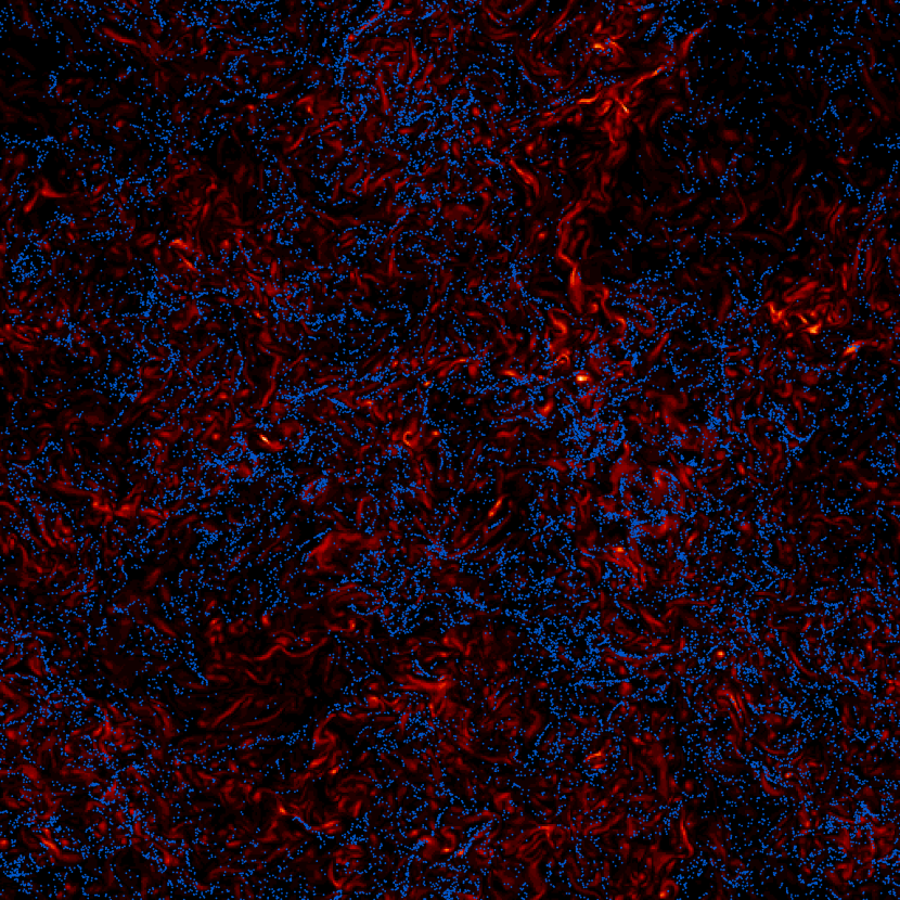
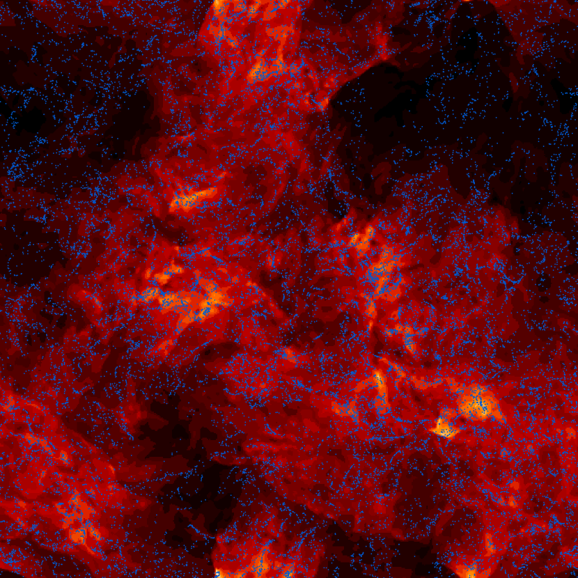
Figure 3.— Flow vorticity (left panel) and density(right panel) on a slice of the simulation box. The thickness of the slice is two computational zones. The color scale is linear with vorticity or density, and the red color represents high vortcity or density values. Blue dots are locations of particles with $St=1.2$. A clear anti-correaltion is seen between the vorticity field and the particle positions, whereas the particle distribution is independent of the flow density. The total number of particles is the same in the two panels. The impression that the left panel has more particles than in the right panel is due to the color contrast.

In our transonic flow, we find that particles are clustered with statistical properties very similar to those in incompressible flows. The particle clustering found here is not due to the compressibility of the gas flow, because very strong particle concentration enhancement exists after compensating the flow compressibility by dividing the particle number density by the flow density. The strongest clustering is indeed found for particles with $St\sim 1$. Much smaller particles (with much shorter friction timescale) behave essentially like tracer particles, and do not show any clustering relative to the gas. Clustering of larger particles is also weaker and occurs at larger scales. Fig. 2 shows the position of all the particles with $St=1.2$ and $St=4.9$ within a slice of thickness equal to 2% of the computational box. At large scales, the spatial distribution of the $St=4.9$ particles (right panel) appears to roughly coincide with that of the $St=1.2$ particles (left panel). However, the largest particle densities achieved by the $St=1.2$ particles are much larger than those of the $St=4.9$ particles (this cannot be fully appreciated in Fig. 2, due to the overlap of the particle positions in the densest regions). Furthermore, the $St=1.2$ particles show much more small-scale structure than the $St=4.9$ particles.

The largest particle densities are found in very elongated structures, especially in the case of the $St=1.2$ particles (see Fig. 2). The length of these dense particle filaments approaches the size of the integral length, $L_{1}$, of the flow, which is estimated to be approximately 0.2 times the simulation box size. The integral scale is defined as $L_{1}=3\pi\int k^{-1}E(k)dk/(4\int E(k)dk)$ where $E(k)$ is the energy spectrum. The particle distribution of Fig. 2 is also characterized by large voids, with sizes spanning the whole inertial range up to the $L_{1}$. The statistics of inertial-range-size voids has been studied by Yoshimoto and Goto (2007). The consequences of such dense filaments and voids in the particle distribution have never been studied in the astrophysical literature. We will focus on this important feature of turbulent clustering in a separate work.

In Fig. 3, we plot the flow vorticity and density on a thin slice of the simulation box, with thickness equal to two computational zones, or 5$\eta$. The particle positions are also shown (blue dots). From the left panel, we see that particles are mainly located in between regions with strong vorticity. This is consistent with our physical discussion that inertial particles are expelled by vortices and accumulate in the strain-dominated regions. On the other hand, the particle distribution is generally independent of the flow density, suggesting that particle clustering in our flows are not caused by or significantly affected by compressible modes in our flow.

4. Clustering Statistics of Identical Particles

4.1. The Radial Distribution Function

Figure 4.— Radial distribution functions for particles with $St<1$ (left panel) and $St>1$ (right panel). The Stokes number for each curve is indicated by a nearby label.

Figure 5.— Radial distribution functions at scales $r\;\hbox to0.0pt{\lower 2.5pt\hbox{$\sim$}\hss}\raise 1.5pt\hbox{$<$}\;\eta$. Solid lines are power-law fits. Left and right panels correspond to $St<1$ and $St>1$, respectively. The Stokes number for each curve is indicated by a nearby label.

The spatial distribution of particles can be studied by computing the density correlation function from the particle number density field, $n({\boldsymbol{x}})$. The correlation function is defined as,

$$\xi(St,r)=\frac{1}{\bar{n}^{2}}\langle(n({\boldsymbol{x}})-\bar{n})(n({\boldsymbol{x}}+{\boldsymbol{r}})-\bar{n})\rangle$$ (5)

where $\bar{n}$ is the average particle number density, and $\langle\cdot\cdot\cdot\rangle$ denotes the ensemble average. Alternatively, one can examine the fluctuations in the particle density, $n_{\rm r}$, coarse-grained over different length scales, $r$ (see, e.g., Falkovich and Pumir 2004). The variance, $\langle(\delta n_{\rm r})^{2}\rangle$ (where $\delta n_{\rm r}\equiv n_{\rm r}-\bar{n}$), of the coarse-grained density field as a function of $r$ provides equivalent statistical information as the correlation function $\xi(St,r)$. The two measures can be converted from each other using the correlation-fluctuation theorem (see below).

Here we use another approach based on the counting of particle pairs at given separations. We compute the radial distribution function (RDF hereafter), $g(St,r)$. It is defined such that the average number, $P(St,r)$, of particles in a volume element, $dV$, at a distance, $r(>0)$, from a reference particle is given by,

$$P(St,r)=\bar{n}g(St,r)dV.$$ (6)

This definition is essentially the same as that of the two-point correlation function of galaxies in cosmology (e.g., Peebles 1980). Clearly, for a uniform distribution, $g(St,r)=1$. From their definitions, the RDF is equivalent to the density correlation function, i.e., $g(St,r)=1+\xi(St,r)$ (see Shaw 2003). The measured RDF can be used to calculate the variance, $\langle(\delta n_{\rm r})^{2}\rangle$, of the particle density fluctuations at a given scale $r$ through the correlation-fluctuation theorem. The theorem states that

$$\frac{\langle(\delta n_{\rm r})^{2}\rangle}{\bar{n}^{2}}=\frac{1}{\bar{n}V(r)}+\frac{1}{V(r)}\int_{V(r)}(g(St,r^{\prime})-1)d^{3}r^{\prime}$$ (7)

where $V(r)$ is a volume of size $r$. The derivation of eq. (7) can be found in, e.g., Landau & Lifshitz (1980) and Peebles (1980). The first term on the r.h.s. is the reciprocal of the average particle number in $V(r)$ and corresponds to the effect of shot noise (Poisson process). The term is negligible for the case of dust particles at length scales, $r$, of astrophysical interest. If $\xi(St,r)$ or $g(St,r)$ is a power law function of $r$, as found to be the case at $r<\eta$ (see below), we have $\langle(\delta n_{\rm r})^{2}\rangle\simeq\bar{n}^{2}\xi(St,r)$.

The RDF is especially useful in estimating the collision kernel for particle coagulation models. The kernel is proportional to $\bar{n}^{2}g(St,d_{\rm p})\delta v(St,d_{\rm p})$, where $\delta v(St,d_{\rm p})$ is the particle relative speed at a distance of the particle diameter $d_{\rm p}=2a_{\rm p}$ (Wang et al. 2000). Both clustering and turbulence-induced relative speed tend to increase the particle collision rate.

For our simulation data, computing the RDF is a better approach than the statistical measures based on the particle density. This is because the number of particles in our simulations is limited, and, at small scales, the particle density may not be evaluated with high accuracy. On the other hand, we find that the number of particles is enough to provide sufficient statistics for the RDF well below the Kolmogorov scale, $\eta$ (see Fig. 5).

Figure 6.— Scaling exponent, $\mu(St)$, of the RDFs in the dissipative range. Error bars show the measurement uncertainty ($\pm 3\sigma$).

Fig. 4 shows our numerical results for the radial distribution function, $g(St,\tilde{r})$, as a function of the particle separation normalized to the Kolmogorov scale, $\tilde{r}\equiv{r/\eta}$, for different Stokes numbers. The left panel plots the RDFs for $St=0.08$, 0.16, 0.31, 0.62 from bottom to top. The RDF increases with the Stokes number at all scales, and this monotonic increase actually continues to $St=1.2$ (in the right panel). This is in agreement with our discussions in §2.1 for $St\;\hbox to0.0pt{\lower 2.5pt\hbox{$\sim$}\hss}\raise 1.5pt\hbox{$<$}\;1$. For these small Stokes numbers, strong clustering is observed at small scales. Consistent with previous simulation results, we find that, for $r\;\hbox to0.0pt{\lower 2.5pt\hbox{$\sim$}\hss}\raise 1.5pt\hbox{$<$}\;\eta$, $g(St,\tilde{r})$ can be well fit by a power law,

$$g(St,\tilde{r})=C(St)\tilde{r}^{-\mu(St)}.$$ (8)

This is shown in left panel of Fig. 5 where we give the power-law fits (solid lines) to the measured RDF (dashed lines) in the scale range from 0.03 to 2 $\eta$. The exponent $\mu(St)$ increases with $St$ for $St\;\hbox to0.0pt{\lower 2.5pt\hbox{$\sim$}\hss}\raise 1.5pt\hbox{$<$}\;1$ (see Fig. 6). The power-law RDFs at $r\;\hbox to0.0pt{\lower 2.5pt\hbox{$\sim$}\hss}\raise 1.5pt\hbox{$<$}\;\eta$ suggest self-similarity of the particle structures in the dissipation range. On the other hand, at scales $r\;\hbox to0.0pt{\lower 2.5pt\hbox{$\sim$}\hss}\raise 1.5pt\hbox{$>$}\;2\eta$, the RDFs cannot be fit by power laws, meaning that the particle density structures are not self-similar in the inertial range. The curvature of the RDF curves in the inertial range indicates that the clustering process becomes faster and faster as the length scale decreases toward the Kolmogorov scale. The same trend is seen in the $St=1.2$ curve in the right panel.

Figure 7.— RDF as a function of the Stokes number at different length scales.

The clustering behavior for $St\;\hbox to0.0pt{\lower 2.5pt\hbox{$\sim$}\hss}\raise 1.5pt\hbox{$>$}\;1$ are shown in the right panel of Fig. 4. From top to bottom, the solid lines correspond to $St=1.2$, 2.4, 4.9, 10, 21 and 43. The shape of the RDF for $St=1.2$ is very similar to those shown in the left panel. However, starting from $St=4.9$, the curvature of the RDFs is completely different. For these large particles, the RDF first increases steadily toward smaller $r$. As $r$ decreases further, a clear decrease in the RDF slope occurs at an inertial-range scale for $St\geq 4.9$. The scale at which the RDF starts to flatten increases with the Stokes number. Below that scale, the RDF becomes essentially flat for $St\;\hbox to0.0pt{\lower 2.5pt\hbox{$\sim$}\hss}\raise 1.5pt\hbox{$>$}\;10$, suggesting that no significant particle density fluctuations exist at these scales. This is in agreement with our physical discussion. In §2.2, we argued that large particles cluster mainly at a scale, $l_{\tau_{\rm p}}$, and, below $l_{\tau_{\rm p}}$, the particle relative motions are random, and no further clustering occurs. This explains the flat part in the RDFs of $St\gg 1$ particles. Therefore, the scale at which the RDF flattens corresponds to $l_{\tau_{\rm p}}$, which increases with $\tau_{\rm p}$ as $\tau_{\rm p}^{3/2}$ for $\tau_{\rm p}$ in the inertial range. This predicts that the scale for the RDF slope change goes like $St^{3/2}$. Unfortunately, due to the limited numerical resolution, it is not clear if this scaling is strictly obeyed. In the inertial range, the clustering intensity of large particles can be significantly larger than that of small particles with $St\simeq 1$, as can be seen from a comparison of the $St=1.2$ RDF to the $St=4.9$, $10$, $21$ curves in the scale range from $5\eta$ to $50\eta$. The study of turbulent clustering at inertial-range scales of astrophysical systems should thus pay particular attention to large particles with $St\gg 1$.

In the right panel of Fig. 5, we plot the RDFs in the scale range from 0.03 to 2$\eta$ for $St>1$ particles. As in the $St<1$ case, they can also be fit by power-laws (solid lines). The RDF slope decreases with $St$ in this Stokes number range, and the RDF for $St\geq 10$ is completely flat. In Fig. 6, we show the scaling exponent $\mu(St)$ as a function of $St$, which peaks at $St=0.63$.

In Fig. 7, we plot the RDF as a function of the Stokes number at six length scales. The RDF decreases with increasing length scale. At scales below $\eta$, the degree of clustering strongly peaks at $St\sim 1$. The peak systematically moves to larger Stokes numbers as the length scale $r$ becomes larger than $\eta$. As discussed above, the strongest clustering at the inertial-range scales is from particles with $\tau_{\rm p}$ corresponding to the inertial range.

Our results for the RDF are in good agreement with Collins and Kesiwani (2004), who investigated clustering of $St\sim 1$ particles in incompressible flows using DNS. Fig. 5 of Collins and Kesiwani (2004) shows the exponent $\mu$ measured at different resolutions. The exponent has apparently converged at their highest resolution ($192^{3}$). At that resolution, $\mu$ is around 0.69 for $St=0.4$ and 0.7, and decreases to 0.65 and 0.50 at $St=1$ and $St=1.5$, respectively. These $\mu$ values match very well with our Fig. 6. The agreement provides an important support for the numerical schemes adopted in our study, including the interpolation method for the velocity field at sub-grid scales. It also suggests that our simulation results can be reliably used to explore the clustering statistics in essentially incompressible flows. The coefficient $C(St)$ in Eq. 8 from our simulations is also consistent with Collins and Keswani (2004). The coefficient is equal to the RDF at $r=\eta$, and from the $St=1.2$ curve in our Fig. 4 we have $C\simeq 6.2$ for $St=1.2$. This is close to the measured values ($\sim 6-7$) of $C(St)$ at $St\simeq 1$ from the 192³ run of Collins and Keswani (2004). The agreement also has interesting implications for the Reynolds number dependence of the RDF (§4.3.1).

From Fig. 4, we see extremely strong clustering at very small scales for particles with $St\sim 1$. The RDF keeps increasing with decreasing length scale below $\eta$. From the RDF plot at smaller scales (Fig. 5), we find that the RDF is as large as $50$ at $r\simeq 0.03\eta$ for $St=0.62$. This indicates very strong clustering: the probability of finding another particle across a small distance to a given particle can be enhanced by a factor of $\sim 100$, relative to the case of uniformly distributed particles. The rms concentration, $\langle\delta n_{\rm r}^{2}\rangle^{1/2}/\bar{n}$, at this scale is very large, $\sim 10$.

Particle clustering at small scales can strongly enhance the particle collision rates. This needs to be accounted for in particle coagulation models. As mentioned earlier, the collision rate is proportional to the RDF, $g(St,d_{\rm p})$, at a separation equal to the particle diameter $d_{\rm p}$. The collision frequency is thus $g(St,d_{\rm p})$ times larger than if turbulent clustering is neglected. In other words, turbulent clustering reduces the coagulation/collision timescale by a factor of $g(St,d_{\rm p})$. The particle diameter is usually much smaller than $\eta$, and $g(St,d_{\rm p})$, at $d_{\rm p}$ can be evaluated by extrapolation using our power-law fits at scales below $\eta$.

The increase of the RDF toward the particle size, $d_{\rm p}$, may be suppressed by the Brownian motions of particles. The Brownian motions diffusively spread the particles and tend to smear out the particle density fluctuations. There is a scale below which the Brownian motions dominate over the production of particle fluctuations by turbulent clustering. We will refer to this scale as the Brownian scale and denote it as $l_{\rm B}$. We give a derivation of $l_{\rm B}$ in Appendix B. Below $l_{\rm B}$ no further clustering is expected, and the radial distribution function should be flat. Therefore, if the Brownian scale is larger than the particle diameter, we have $g(St,d_{\rm p})\simeq g(St,l_{\rm B})$, and the extrapolation should stop at $l_{\rm B}$. On the other hand, if $l_{\rm B}\;\hbox to0.0pt{\lower 2.5pt\hbox{$\sim$}\hss}\raise 1.5pt\hbox{$<$}\;d_{\rm p}$, we need to extrapolate the RDF down to $d_{\rm p}$ for the estimate of $g(St,d_{\rm p})$.

In summary, we have measured the RDF for particles of different sizes from our simulation data, and the results are consistent with the physical discussions in §2. Strongest clustering are found to occur at $St\sim 1$. The RDFs in the dissipation-range scales follow power laws and the exponent $\mu(St)$ is largest at $St\simeq 1$. The power-law increase of the RDF toward small scales implies a strong effect of turbulent clustering on the particle collision rate. Large particles ($St>1$) cluster primarily at inertial-range scales, where their clustering intensity is larger than that of $St<1$ particles.

4.2. The Particle Concentration PDF

As a second order statistical measure, the RDF reflects the rms amplitude of the particle density fluctuations. In some applications, high-order statistics, corresponding to clusters with extreme particle density, are of particular interest. For example, in §6 we will discuss planetesimal formation models based on particle clusters of high concentration level in protoplanetary disks. The probability of finding these dense clusters can be estimated from the probability density function (PDF) of the particle concentration.

We will compute the concentration PDF at different length scales. At each length scale, $r$, we consider regions of size $r$, and in each region we define a particle concentration $C\equiv n_{\rm r}/\bar{n}$ where $n_{\rm r}$ is the average number density in that region. We denote as $P_{\rm r}(C)$ the concentration PDF at scale $r$, which represents the probability of finding clusters of size $r$ with a given particle concentration, $C$.

The computation of the PDF from our simulation data is done as follows. We first divide the simulation box into cubes of size $r$ and evaluate the particle number density and the concentration in each cube. The particle density (and hence the concentration) can be accurately measured only if the number of particles in a cube is much larger than 1. We thus decided to only count the cubes containing 4 or more particles, while the cubes with less particles were simply ignored. Therefore, the measured PDF starts from a minimum concentration corresponding to 4 particles per cube. The minimum increases with decreasing length scale $r$ (see Fig. 8) because, for smaller cube sizes, 4 particles per cube implies a larger concentration. Using this method, we computed the concentration PDF down to the scale $\simeq\eta$.

Due to the limited number of particles, the measured PDFs can be contaminated or even dominated by the Poisson noise, especially at small scales. We compared the measured concentration PDF at each scale to the PDF that arises purely from Poisson poise. At small scales ($r\;\hbox to0.0pt{\lower 2.5pt\hbox{$\sim$}\hss}\raise 1.5pt\hbox{$<$}\;5\eta$), we only measured the high tails of the PDF, and the probability in the tails appears to be well above the Poisson noise PDF (by at least two orders of magnitude) for Stokes numbers in the range $0.3\leq St\leq 10$. Particles outside this range are less clustered, and the measured PDFs are close to the Poisson PDF. For those particles, we need a larger number of particles in the simulations to obtain accurate statistics. At large scales ($r\;\hbox to0.0pt{\lower 2.5pt\hbox{$\sim$}\hss}\raise 1.5pt\hbox{$>$}\;10\eta$), we have good measurements for particles with $0.16\;\hbox to0.0pt{\lower 2.5pt\hbox{$\sim$}\hss}\raise 1.5pt\hbox{$<$}\;St\;\hbox to0.0pt{\lower 2.5pt\hbox{$\sim$}\hss}\raise 1.5pt\hbox{$<$}\;40$, whose PDFs are significantly broader than the Poisson PDF.

Figure 8.— Cumulative PDF of the particle concentration for $St=1.2$ particles at different length scales.

In Fig. 8, we plot the cumulative PDF, $P_{\rm r}(>C)=\int_{C}^{\infty}P_{\rm r}(C^{\prime})dC^{\prime}$ at different scales for $St=1.2$. The PDF is broader at smaller scales, corresponding to the increase of the RDF with decreasing length scale at $St\sim 1$. As $r$ decreases toward $\eta$, the broadening of the PDF appears to be faster, consistent with the trend observed in the RDF for $St=1.2$. The scale dependence here is quite sensitive. The PDFs at large scales ($r\gg\eta$) are much narrower than those at small scales.

From Fig. 8, we see that at $1.25\eta$ there is a finite probability of finding regions with very high concentration enhancement, $C\sim 10^{3}$. The trend that the PDF becomes broader with decreasing scale suggests that even higher density clusters may be found at scales below $\sim\eta$. The growth of the PDF tail may continue to the Brownian scale, below which further clustering is suppressed. However, the PDFs shown in Fig. 8 do not account for the back reaction from the particles to the carrier flow, which is not included in our simulations. The back reaction cannot be neglected in regions with $C\;\hbox to0.0pt{\lower 2.5pt\hbox{$\sim$}\hss}\raise 1.5pt\hbox{$>$}\;10^{3}$, because the local mass loading factor $\Phi_{\rm m}$ is much larger than 1 (assuming an average dust-to-gas ratio of 0.01). Therefore, the back-reaction may significantly affect the high tails of $P(C)$ (Hogan and Cuzzi 2007). This will be discussed in more details in §4.5.

Following Hogan et al. (1999), we also considered the PDF with mass-weighting, $P_{\rm m}(C)$, which is related to the volume-weighted PDF, $P(C)$, by $P_{\rm m}(C)=CP(C)/\langle C\rangle$ (here the subscript “r” for the scale dependence is dropped for simplicity of the notation). The cumulative PDF with mass-weighting is thus $P_{\rm m}(>C)=\int_{C}^{\infty}C^{\prime}P(C^{\prime})dC^{\prime}/\langle C\rangle$, which is the fraction of the total number (or mass) of particles experiencing a concentration larger than $C$. The cumulative mass-weighted PDF is plot as dotted lines in Fig. 8. We find that that the volume- and mass- weighted PDF tails at $r=2.5\eta$ in our Fig. 8 are quite close to the results in Hogan et al. (1999) (their Fig. 3c and 3d, respectively) for $St=1$ particles at $r=2\eta$ in a $Re_{\lambda}=140$ flow. The cumulative PDF with mass-weighting has much broader tails. For example, the PDF tails at $r=\eta$ in our Fig. 8 show that the mass-weighted probability for $C\;\hbox to0.0pt{\lower 2.5pt\hbox{$\sim$}\hss}\raise 1.5pt\hbox{$>$}\;10^{3}$ is about $10^{3}$ times larger than the volume-weighted one. We note that the PDFs shown in Fig. 4 of Cuzzi et al. (2001) and in Fig. 1 of Cuzzi et al. (2008) correspond to the mass-weighted cumulative PDFs in Fig. 3d of Hogan et al. (1999).

Although our Fig. 8 looks similar to Fig. 1 in Cuzzi et al. (2008), they are different. In our figure, the particle size and numerical resolution are fixed, the curves correspond to different length scales. On the other hand, Fig. 1 of Cuzzi et al. (2008) shows the concentration PDFs at different numerical resolutions with the Stokes number and the normalized length scale fixed at $St\simeq 1$ and $\tilde{r}=2$ respectively.

Figure 9.— Cumulative PDF of the particle concentration at $r=10\eta$. At this scale the PDF width peaks at $St=4.9$. For larger $St$, the PDF becomes narrower. The dotted line shows the PDF of Poisson noise.

We also computed the concentration PDFs for other Stokes numbers. At a given scale, the PDF tails as a function of $St$ have a similar behavior as the RDFs shown in Fig. 7. At $r\simeq\eta$, the PDF tail first broadens with increasing $St$, and reaches a maximum width at $St\simeq 1$. As $St$ increases further, the PDF tail becomes narrower. Also consistent with the RDF in Fig. 7, the Stokes number at which the PDF width reaches maximum becomes larger with increasing length scale. For example, at $r=10\eta$ and $40\eta$, the PDF tail reaches maximum at $St=4.9$ and $10$, respectively. Again the highest clustering intensity at inertial-range scales is from particles with $\tau_{\rm p}$ in the inertial range. In Fig. 9, we show the dependence of the PDF tail on $St$ at the scale $r=10\eta$. Starting from $St=4.9$ where the PDF has the maximum width, the tail becomes narrower as $St$ increases. At $St\;\hbox to0.0pt{\lower 2.5pt\hbox{$\sim$}\hss}\raise 1.5pt\hbox{$>$}\;93$, the PDF is quite close to the Poisson PDF, indicating only a slight or negligible clustering effect.

4.3. Reynolds number dependence

Currently available numerical studies are far from resolving scales around the turbulence dissipation scale, $\eta$, in interstellar clouds or protoplanetary disks, as the characteristic Reynolds number in these astrophysical systems is $Re\;\hbox to0.0pt{\lower 2.5pt\hbox{$\sim$}\hss}\raise 1.5pt\hbox{$>$}\;10^{6}$. The possible dependence of the clustering properties on the Reynolds number must be carefully examined, if results of numerical simulations are to be applied to astrophysical environments.

The $Re$ dependence is usually discussed in a unit system where the length scale and the particle friction timescale are normalized, respectively, to the Kolmogorov length and time scales in the carrier flow. Numerical simulations used to study the $Re$-dependence usually keep the large-scale properties (such as the rms velocity and the integral length scale) roughly constant, and decrease the viscosity (and hence the Kolmogorov scale) with increasing resolution. In the statistical analysis, these studies normalize all the quantities to the smallest scales (i.e., $\eta$ and $\tau_{\eta}$) in the simulated flows, and examine how the clustering properties at given $St$ and $\tilde{r}$($\equiv r/\eta$) change with the Reynolds number. Note that, in the comparison of the clustering statistics in simulated flows with the same large-scale properties, but different $Re$, given values of $St$ and $\tilde{r}$ correspond to different particle sizes (i.e., different $\tau_{\rm p}$) and different actual length scales, $r$ (larger particle size and length scale in the lower $Re$ flow).

The Reynolds number dependence of particle clustering has been discussed in a number of numerical studies using simulations at different resolutions (e.g., Hogan, Cuzzi and Dobrovolskis 1999, Wang et al. 2000, Reade and Collins 2000a, Hogan and Cuzzi 2001, Falkovich and Pumir 2004, Collins and Keswani 2004). Here we give a brief summary of the results from these studies.

4.3.1 Reynolds number Dependence of the RDF

The RDF was found to increase with $Re$ at very low $Re$. Wang et al. (2000) computed the RDF at $r=\eta$ in four simulated flows with the Taylor Reynolds number, $Re_{\lambda}$, in the range from 24 and 75. Their results show that the RDF increases linearly with $Re_{\lambda}$ (i.e., by a factor of 3 as $Re_{\lambda}$ goes from 24 to 75), and that the shape of $g(St,\tilde{r}=1)$ as a function of $St$ does not change with $Re_{\lambda}$ (see also Hogan and Cuzzi (2001)). A similar increase in the RDF with increasing $Re_{\lambda}$ is observed by Reade and Collins (2000a) for $r=0.025\eta$ in a similar range of $Re_{\lambda}$.

At higher resolutions, different conclusions were obtained in different studies. Using numerical simulations with $Re_{\lambda}\;\hbox to0.0pt{\lower 2.5pt\hbox{$\sim$}\hss}\raise 1.5pt\hbox{$<$}\;130$, Falkovich and Pumir (2004) found that the scaling exponent, $\mu(St)$, for $St<1$ at $r<\eta$ has a significant increase with increasing $Re_{\lambda}$. This dependence has been suggested to have important implications for the growth of droplets in terrestrial clouds. On the other hand, Collins and Keswani (2004), who explored $St\sim 1$ particles in a similar $Re_{\lambda}$ range (up to 152), showed that the scaling exponent, $\mu(St)$, is essentially independent of $Re_{\lambda}$, and that the coefficient, $C(St)$, first increases with $Re_{\lambda}$ at small $Re_{\lambda}$, and then converges to a constant at $Re_{\lambda}=152$. These suggest that the RDF may be $Re$ independent at sufficiently large $Re$. In §4.1, we found that the RDF of $St\simeq 1$ particles in our simulated flow with $Re_{\lambda}\simeq 300$ are in good agreement with Collins and Keswani (2004). This supports the claim by Collins and Keswani (2004) that the RDF is $Re$-independent at high Reynolds numbers. However, we think that a conclusive answer to the $Re$ dependence of the RDF still needs confirmation from simulations of higher-resolutions.

The $Re$ dependence of the RDF of $St>1$ particles in the inertial range has not been investigated. These large particles cluster at a scale, $l_{\tau_{\rm p}}$, in the inertial range, which were barely resolved in existing studies. To accurately capture the clustering statistics at the scale $l_{\tau_{\rm p}}$, an extended separation between $l_{\tau_{\rm p}}$ and the low outer scale, $L$, is needed, where the RDF increases toward smaller scales (see Fig. 4). This requires even higher numerical resolutions than for the study of $St\;\hbox to0.0pt{\lower 2.5pt\hbox{$\sim$}\hss}\raise 1.5pt\hbox{$<$}\;1$ particles. We speculate that the $Re$ dependence for $St>1$ particles would be weaker than that for $St\;\hbox to0.0pt{\lower 2.5pt\hbox{$\sim$}\hss}\raise 1.5pt\hbox{$<$}\;1$ particles. In §2.1, we showed that, for $St<1$, the divergence of the particle flow is proportional to the velocity gradient squared, which has a fairly strong $Re$ dependence. In contrast, the effective compressibility estimated for particles in §2.2 does not depend on the flow properties. Therefore the $Re$ dependence for $St>1$ particles is expected to be weaker. If the RDF of $St\;\hbox to0.0pt{\lower 2.5pt\hbox{$\sim$}\hss}\raise 1.5pt\hbox{$<$}\;1$ particles is $Re$-independent at large $Re$, the same is probably also true for $St>1$. Future numerical studies can test this speculation.

4.3.2 Reynolds Number Dependence of the PDF

In §2.1, we derived the divergence of the particle flow for $St\;\hbox to0.0pt{\lower 2.5pt\hbox{$\sim$}\hss}\raise 1.5pt\hbox{$<$}\;1$, and found that the divergence has a quadratic dependence on the flow velocity gradient. The PDF of the velocity gradient in a turbulent flow is known to broaden with increasing $Re$. The same is thus expected for the PDF of the particle flow divergence, meaning that the probability of strong compressing or expanding events is higher at larger $Re$. As a consequence, the concentration PDF for $St\;\hbox to0.0pt{\lower 2.5pt\hbox{$\sim$}\hss}\raise 1.5pt\hbox{$<$}\;1$ particles is likely to become broader with increasing Reynolds number. Note that a $Re$-dependent PDF does not suggest that the RDF, a second-order statistical measure, must also depend on $Re$. It is possible that the tails of a PDF broaden considerably with $Re$, while the second order moment is constant.

Broadening of the particle concentration PDF with increasing resolution was found in the numerical study of Hogan et al. (1999) for particles with $St=1$. Hogan et al. (1999) carried out a multifractal analysis of the particle concentration field that can be used to extrapolate the PDFs measured from low-$Re$ simulations to realistic values of $Re$. They computed the singularity spectra of the particle concentration field at different scales ($2\leq\tilde{r}\leq 8$), in simulations with three different values of $Re$. Fig. 2 of Hogan et al. (1999) shows that, at each Reynolds number, the spectra are different at different scales, indicating that the particle density structures are not self-similar at scales above $2\eta$. This is consistent with our observation that the RDF is not a power-law at scales above $2\eta$ in our simulations. Strictly speaking, the scale dependence of the singularity spectrum means that the particle structures are not “fractals”. However, the multifractal analysis provides useful information on how the clustering process proceeds with decreasing length scales. The singularity indices are significantly smaller at smaller scales, suggesting the development of strong particle density structures becomes faster and faster toward smaller $r$.

On the other hand, the singularity spectra at a given scale, $\tilde{r}$, are found to be independent of the Reynolds number. Based on this dependence, Hogan et al. (1999) gave a model to extrapolate the concentration PDF from simulation results to that at realistic Reynolds numbers. Applying the extrapolation to $Re$ values typical of turbulence in planetary disks, Cuzzi et al. (2001) found a significant probability of finding regions (of size $\sim\eta$ ) with extreme concentration enhancement ($C\sim 10^{4}-10^{5}$).

The singularity spectrum of the particle concentration at $2\eta$ measured by Hogan et al. (1999) is very similar to that of the dissipation rate in the turbulent flow (see their Fig. 2). The reason is probably that the particle velocity divergence has a quadratic dependence on the flow velocity gradient, which is similar to that of the dissipation rate.

Hogan et al. (1999) only investigated particles with $St\sim 1$, and the $Re$ dependence of the concentration PDF at $St<1$ or $St>1$ has not been studied. We expect that the concentration PDF of small particles ($St<1$) would broaden with increasing $Re$ in a similar way as $St\sim 1$ particles, because the divergence of these particles has a similar dependence on the velocity gradients. It is unknown how the concentration PDF of $St>1$ particles changes with $Re$. As in the RDF case, we argue that, in the $St>1$ case, the $Re$ dependence of the concentration PDF would be weak in comparison to the $St\sim 1$ particles. This is again based on our observation in §2.2 that the effective compressibility ($\sim 1/\tau_{\rm p}$) of large particles at the clustering scale $l_{\tau_{\rm p}}$ does not show an explicit dependence on the flow velocity gradients or velocity differences.

4.4. Interpretation of Simulation Results

Due to the limited numerical resolution, the Kolmogorov timescale in simulated flows is usually much larger than that in a real flow. The Stokes number of a particle of a given size would be much smaller in a simulation than in the real flow. A consequence of this mismatch of the Stokes numbers is that the clustering intensity from a simulation may not correctly reflect that in the real situation, as the clustering statistics have a quite sensitive dependence on $St$. Therefore, simulation results involving the clustering properties of inertial particles need to be interpreted with caution.

We discuss how the clustering statistics obtained in simulations may differ from that in the real flow, based on the RDF shown in our Fig. 7. This can be examined from the three correction steps given below, which allow us to see how the real RDF compares to that from a simulation. We use the subscript “n” to denote the numerical results, and the subscript “r” for the real flow.

First, for a given length scale $r$, $\tilde{r}_{\rm r}$ in the real flow is larger than $\tilde{r}_{\rm n}$ in the simulated flow. This shifts the RDF in Fig. 7 toward lower values of $g$ (larger $\tilde{r}$). Second, the Stokes number is larger in the real flow than in the simulation. This corresponds to a shift to the right side along the RDF curve. If $St_{\rm n}\ll 1$ and the shift moves $St$ closer to unity, this correction could give an increase in the clustering strength. On the other hand, if $St_{\rm n}\;\hbox to0.0pt{\lower 2.5pt\hbox{$\sim$}\hss}\raise 1.5pt\hbox{$>$}\;1$, the shift would result in smaller values of $g$. Finally, we need to account for the possible Reynolds number dependence. The Reynolds number is larger in the real flow and, if it exists, the $Re$ dependence would move the RDF curves upward (see §4.3.1).

We consider a specific example where the actual particle size has $St_{\rm r}\gg 1$ in the real flow, but by coincidence corresponds to $St_{\rm n}\sim 1$ in the simulated flow. This example is interesting for our discussion on the planetesimal formation model in §6.3. In this case, the first two steps discussed above would give a clustering intensity much lower than in the simulated flow. In particular, the effect of the $St$ correction, is quite strong, as the RDF curves in Fig. 7 decrease very rapidly with increasing $St$ (for $St>1$). Therefore, the RDF measured in the simulation would overestimate that in the real flow by a large amount, unless there is a strong $Re$ dependence. The same argument can be made for the width of the concentration PDF tails. The $Re$ dependence to be applied here is that for the clustering of $St>1$ particles at inertial-range scales, which has not been studied. In §4.3.1 and 4.3.2, we argued that the $Re$ dependence for these particles is likely to be weak. Therefore the $Re$ dependence may not be able to compensate the decrease in $g$ resulting from the first two corrections. We thus conclude that, if in a simulation the particle Stokes number has an artificial value close to unity, the clustering intensity of those particles may be significantly overestimated. This needs to be considered when interpreting results from astrophysical simulations.

4.5. Back Reaction

We have only considered the effect of the turbulent flow on the inertial particles, but neglected the dynamical effect of the inertial particles on the carrier flow. As shown in our simulations, turbulent clustering can give rise to regions with particle concentration enhanced by a factor of $10^{3}$ (see Fig. 4), leading to local particle densities even larger than the flow density. In these regions, the feedback effect from the mass loading is not negligible, and a discussion of the two-way interactions between the particles and the flow is needed.

The modulation of the carrier flow by the back reaction from the particle phase has been shown to depend on the particle size. Different results have been found for $St<1$ particles and $St>1$ ones, concerning how the back reaction changes the turbulent kinetic energy, how the kinetic energy transfers between the flow and particle phases, and how the energy spectrum of the flow is affected by the two-way coupling (Sundaram and Collins 1999, Boivin, Simonin and Squires 1998, Ferrante and Elghobashi 2003, Shotorban and Balachandar 2009).

Here we are more interested in the effect of the two-way coupling on the clustering intensity. From brief discussions in Sundaram and Collins (1999) (for $St>1$) and in Shotorban and Balachanar (2009) (for $St<1$), we see that including the back reaction gives only a slight change ($\;\hbox to0.0pt{\lower 2.5pt\hbox{$\sim$}\hss}\raise 1.5pt\hbox{$<$}\;10\%$) in the RDF and the particle concentration variance. It seems that the 2nd order clustering statistics is not significantly affected by the back reaction if the rms mass loading factor is smaller than 1. A systematic study of the effect of two-way coupling on the RDF is needed to confirm if this is indeed the case.

On the other hand, the particle feedback can considerably affect the tails of the particle concentration PDF because clusters of high concentration levels induce much larger mass loading than the average. Hogan and Cuzzi (2007) studied the back-reaction effect on the concentration PDF for particles with $St=1$. They built up a model assuming that the development of the fluctuations in the particle concentration and the flow enstrophy (defined as vorticity squared, $\omega^{2}$) can be described as a joint cascade process. In the model, a flow parcel breaks up into two equal-sized subdivisions in each cascade step, and the partitioning of the particle concentration and the flow enstrophy in the two subdivisions is controlled by a probability distribution, called the multiplier PDF. Hogan and Cuzzi (2007) computed the multiplier PDF for the step from $3\eta$ to $1.5\eta$ in their simulations, and found that the multiplier PDF becomes narrower as the mass loading factor, $\Phi_{\rm m}$, exceeds $\sim 10$. When $\Phi_{\rm m}$ becomes larger than $\sim 100$, the multiplier PDF is essentially a delta function, meaning that the bifurcation of the particle density stops in these highly loaded regions. This sets an upper limit for the concentration enhancement: the particle density cannot exceed 100 times the flow density. In short, the back reaction from particles has been found to suppress the probability of forming particle clusters with extreme concentration enhancements.

The two-way interactions between the dust particles and the turbulent flow give rise to an interesting phenomenon in differentially-rotating circumstellar disks. Youdin and Goodman (2005) found that, with two-way coupling, the presence of a radial pressure gradient in such disks leads to an instability, named the streaming instability. They suggested that the instability can produce local particle overdensities, which may help the formation of planetesimals. The simulations by Youdin and Johansen (2007) confirmed the instability and its clumping effect. Johansen and Youdin (2007) showed that, in the saturation stage of the instability, the effect is most prominent for marginally coupled particles with friction timescales close to the rotation period of the disk.

Johansen et al. (2007) showed that including the particle feedback amplifies the maximum concentration from particle clustering by the MRI-driven turbulence in circumstellar disks. It suggests that the streaming instability from two-way coupling gives enhanced clustering strength in such disks. This appears to be different from the case of isotropic turbulence where the particle feedback reduces the high tails of the concentration PDF. (We note, however, that the maximum particle density does not exceed 100 times the flow density in the simulations of Johansen et al. (2007) with no self-gravity). The amplification in the clustering intensity by the streaming instability was important for the planetesimal formation model of Johansen et al. (2007). A more detailed discussion of their model will be given in §6.3.

5. Clustering Statistics of Particles of Different Sizes

So far we have only studied clustering of particles of the same size. In this section, we consider the relative spatial distribution of different particles. As mentioned earlier, the particle clustering location shifts in space as the particle size changes. This has interesting consequences for the clustering statistics of particles of different size. We quantify this effect by analyzing our simulation data.

5.1. The Bidisperse RDF

We first compute the bidisperse RDF, $g(St_{1},St_{2},r)$, for two different particles with Stokes numbers $St_{1}$ and $St_{2}$, which is defined as the probability of finding a particle with $St_{2}$ (or $St_{1}$) at a distance $r$ from a reference particle with $St_{1}$ (or $St_{2}$). The computation is done in a similar way as for the mondisperse case. The RDF for the bidisperse case is equivalent to the two-point cross correlation function for the (number) density fields of two different particles.

Fig. 10 shows the bidisperse RDF as a function of the length scale for different Stokes number paris. One of the Stokes numbers is fixed at $St_{1}=1.2$, and the dotted line is the monodisperse RDF with $St=1.2$. We see that, at large scales, the bidisperse RDF is close to the monodisperse one. This is because the particle clusters are generally located at the same regions when viewed at these large scales. With decreasing length scale, the bidisperse RDF becomes flat, consistent with results by Reade and Collins (2000b) and Zhou et al. (2001). This indicates the density fields of the two different particles become less correlated at smaller scales. The spatial separation between clustering locations becomes visible when examined at small scales. The length scale at which the RDF flattens increases as the ratio of the particle sizes increases, corresponding to a larger separation between the clustering positions of the two particles. Similar behaviors have been found for the bidisperse RDFs with other values for the fixed Stokes number $St_{1}$. Chun et al. (2005) showed that the flattening trend exists as long as there is a difference in the particle sizes. Even if the Stokes numbers difference is small, one still finds a flat part of the RDF when going to sufficiently small scales, due to the finite (but small) shift in the clustering locations. This result suggests that, in the bidisperse case, the clustering effect contributes less to the particle collision rates than in the monodisperse case.

Figure 10.— Bidisperse RDF for different Stokes number pairs. One of the Stokes numbers, $St_{1}$, is fixed at 1.2. The dotted line is the monodisperse RDF for $St=1.2$. Thinner lines are used to plot RDFs with $St_{2}$ farther away from $St_{1}$.

In Fig. 11, we show the bidisperse RDF as a function of $St_{2}$. The other Stokes number $St_{1}$ is fixed at 1.2. Different curves correspond to different length scales. For $\tilde{r}\sim 1$, the bidisperse RDF peaks at $St_{2}\sim St_{1}$, and decreases rapidly as the Stokes number ratio increases. The RDF is significantly reduced as the ratio increases to 3, and the density fields are essentially uncorrelated when the Stokes number ratio is larger than 10. At larger length scales, the RDF peak moves to the right. This is because at these scales ($r\gg\eta$) large particles ($St>1$) have stronger density fluctuations than the smaller ones ($St<1$).

Figure 11.— Bidisperse RDF at six length scales. $St_{1}$ is fixed at $1.2$.

In summary, we found the bidisperse RDF becomes flat at small scales because particles of different sizes tend to cluster at different places. The bidisperse RDF decreases with increasing particle size ratio, and the effect of clustering on the particle collision rates between different particles is weaker than in the mondisperse case. The overall fluctuation amplitude of the particle density may be significantly suppressed if the particle size spanned an extended range.

5.2. The Concentration PDF for Multiple Particle Sizes

In Fig. 12, we show the concentration PDFs for two combinations of different particles with $St$ centered around $1.2$. For comparison, we also plot the PDF for the monondisperse case with $St=1.2$ (the dotted line). The dashed lines and the solid lines correspond to the results for combinations of 3 and 5 different particle sizes, respectively. The concentration factor shown in Fig. 12 represents the enhancement in the total number density in local regions relative to the average. When computing $C$ in each local region, we obtained the local number density by counting the total number of particles with size in the chosen range and then divided it by the average. Each particle size was given the same weighting factor as we have the same number of particles for each size in our simulations. The concentration $C$ computed this way can be understood as the enhancement factor in the particle mass density if the particle size distribution is such that the total mass of particles of each size is the same. Fig.  12 is just an illustration of how the concentration PDF changes in the presence of multiple particle sizes. For practical applications, one needs to use the proper weighting factor for each size according to the actual size distribution.

At $r=1.25\eta$, the PDF moves toward significantly smaller $C$, as the particle size range increases. There are two reasons for the behavior. First, at scales $\sim\eta$, the degree of clustering for each individual size decreases as the Stokes number gets farther from $1.2$. Including particles with $St$ larger or smaller than 1 leads to weaker overall clustering. Second, the bidisperse RDFs in Fig. 10 show that if the Stokes number ratio of two particles is larger than 2, their clustering locations do not overlap at length scales $r\sim\eta$. This means that different particle sizes chosen in Fig. 12 essentially occupy different places when we look at scales $\sim\eta$. This has the effect of smoothing out the fluctuations in the overall particle density distribution, giving narrower PDF tails. The maximum $C$ in the measured PDFs at $r=1.25\eta$ and $2.5\eta$ for the 5-particle case is smaller than the monodisperse case (dotted line) by a factor of $4-5$. This confirms that the strongest clusters of the 5 particles are spatially separated, with the typical separation larger than $\sim\eta$. The shift of the PDF tail toward smaller $C$ implies that the probability of finding particle clusters of extreme concentration level is greatly reduced if the particle size has an extended range. Therefore, using a single typical (or average) particle size to approximate a size distribution could significantly overestimate the clustering intensity.

Figure 12.— The cumulative concentration PDF at different length scales for multiple particle sizes. The dotted line corresponds to the monodisperse case with $St=1.2$, and the dashed and solid lines are for three and five particle sizes, respectively.

As the length scale increases, the shift of the PDF tail becomes smaller, and at $r=40\eta$ the tail is essentially unchanged. One reason is that the clustering locations of these particles overlap when viewed at $r=40\eta$ (see Fig. 10 and the discussion in §5.1). Also unlike the case of small scales ($r\;\hbox to0.0pt{\lower 2.5pt\hbox{$\sim$}\hss}\raise 1.5pt\hbox{$<$}\;\eta$) where the clustering intensity peaks at $St\simeq 1$, at $r=40\eta$ the clustering strength for particles of each individual size keeps increasing as $St$ increases from 0.31 to 4.9 (see Fig. 7). Therefore, the clustering intensity of larger particles (i.e., $St=2.4$, $4.9$) and smaller particles (i.e., $St=0.31$, $0.62$) is, respectively, higher and lower than that from particles of average size ($St=1.2$), and their contributions to the overall clustering can compensate each other. This explains why the PDF at $40\eta$ is almost unchanged.

We also computed the concentration PDFs for combinations of particle sizes centered around $St=10$. In that case, we found that the PDF at $40\eta$ for a combination of 5 different particles with $St=2.4,4.9,10,21$ and $43$ is significantly narrower than the monodisperse PDF for $St=10$. The effect of the existence of multiple particle sizes on the overall clustering intensity at a given scale depends on both the average particle size and the width of the size distribution. The effect can be understood by considering whether the clustering locations of these particles overlap and how much each individual size contributes to the overall clustering.

To summarize, we find that the presence of an extended particle size range tends to reduce the overall clustering intensity, and a careful consideration for the particle size distribution is needed to obtain an accurate estimate for the overall clustering intensity.

6. Application to Protoplanetary Disks

Turbulent clustering of inertial particles has potential applications to dust particles in many astrophysical environments, such as the interstellar medium, protoplanetary disks, and the atmospheres of planets and dwarf stars. As mentioned earlier, clustering of dust grains may significantly increase their collision rates for particles of similar sizes, and thus needs to be considered in coagulation models. Here we will consider clustering of dust particles in protoplanetary disks and, in particular, its role in models for planetesimal formation. Applications to different environments may require exploring other complexities. For example, a study of dust grain dynamics in interstellar clouds needs to account for the Lorenz force due to the electrical charges on the grain surface and the presence of magnetic fields in the clouds.

Preferential clustering of inertial particles in turbulence has attracted attention from the community of planet formation because it may provide a possible solution to the long-standing problem of planetesimal formation. As mentioned in the Introduction, the classic planetesimal formation theory is challenged by the self-generated turbulent stirring, and growth of dust particles to kilometer size by collisional coagulation suffers from the meter-size barrier. Two potential solutions to this problem have been recently proposed by Johansen et al. (2007) and by Cuzzi et al. (2008). The model model by Cuzzi et al. (2008) is directly based on turbulent preferential clustering. Particle clumping in the simulations of Johansen et al. (2007) may also have contribution from turbulent clustering. Before discussing these models, we first consider the properties of turbulence in protoplanetary disks.

6.1. Turbulence in Protoplanetary Disks

Following Cuzzi et al. (2001), we use the $\alpha$ prescription for turbulence in the disks, i.e., the turbulent viscosity, $\nu_{\rm t}$, is parametrized as $\nu_{\rm t}=\alpha C_{\rm s}H$. An $\alpha$ value in the range of $10^{-3}$ to $10^{-5}$ is consistent with observations (see discussions in Cuzzi et al. 2001, 2008). The scale height, $H$, of the disk is given by $H\simeq C_{\rm s}/\Omega_{\rm K}$ with $\Omega_{\rm K}$ being the Keplerian rotation frequency. The turbulent viscosity can be estimated from the turbulent rms velocity, $U$, and the integral scale, $L$, by $\nu_{\rm t}\simeq UL$. Assuming the turnover time, $\sim L/U$, of the largest turbulent eddies is of the order of $\sim\Omega_{\rm K}^{-1}$ (Cuzzi et al. 2001), we have $U=\alpha^{1/2}C_{\rm s}$ and $L=\alpha^{1/2}H$.

We assume a standard minimum-mass solar nebula where the density and temperature profiles are given by $\rho_{\rm g}=1.7\times 10^{-9}(R/\rm{AU})^{-2.75}$ g cm^-3 and $T=280(R/\rm{AU})^{-0.5}$ K. With these scalings, we find $U=10^{3}\alpha_{-4}^{1/2}(R/\rm{AU})^{-0.25}$ cm/s, and $L=5\times 10^{4}\alpha_{-4}^{1/2}(R/\rm{AU})^{1.25}$ km, where $\alpha_{-4}\equiv\alpha/10^{-4}$. To calculate the Kolmogorov scales, we need to estimate the molecular viscosity, $\nu$. Assuming a cross section of $2.5\times 10^{-15}$ cm² for hydrogen molecules, we have $\nu=5\times 10^{4}(R/\rm{AU})^{2.5}$ cm²/s. We then obtain $\eta=5\times 10^{3}\alpha_{-4}^{-1/4}({R}/{\rm{AU}})^{2.38}$ cm, and $\tau_{\eta}=5\times 10^{2}\alpha_{-4}^{-1/2}({R}/{\rm{AU}})^{2.25}$ s. The friction timescale is given by $\tau_{\rm p}=6\times 10^{3}({a_{\rm p}}/{\rm{cm}})({R}/{\rm{AU}})^{3}$ s, where we assumed the density of the dust material is $\rho_{\rm d}=1$ g cm^-3 and used the formula, eq. (2), for the Epstein regime. Finally, we find the Stokes number is $St=12({a_{\rm p}}/{\rm{cm}})({R}/{\rm{AU}})^{3/4}$. Therefore, at 1 AU, the particle size with most intense turbulent clustering ($St\simeq 1$) is $a_{\rm p}\simeq 0.1\alpha_{-4}^{-1/2}$ cm.

In our discussions below on planetesimal formation models, we will take the radius 5 AU as an example. Using the formulas given above, we find $U=7\alpha_{-4}^{1/2}$ m s^-1 and $L=4\times 10^{5}\alpha_{-4}^{1/2}$ km at 5 AU. The Kolmogorov length and time scales are, respectively, $\eta\simeq 2\alpha_{-4}^{-1/4}$ km and $\tau_{\eta}\simeq 2\times 10^{4}\alpha_{-4}^{-1/2}$ s. The friction timescale is given by $\tau_{\rm p}=8\times 10^{5}({a_{\rm p}}/{\rm{cm}})$ s, and we have the Stokes number $St=40\alpha_{-4}^{1/2}(a_{\rm p}/{\rm cm})$. Therefore, at 5 AU the particle size corresponding to $St=1$ is $a_{\rm p}=0.025\alpha_{-4}^{-1/2}$ cm.

As summarized by Brauer, Dullemond, and Henning (2008) and others, theoretical disk models, millimeter-wavelength observations, as well as a careful reevaluation of the minimum mass solar nebular by Davis (2006) all find radial density profiles flatter than the conventional -3/2 power law. Brauer, Dullemond, and Henning (2008) adopt $\rho_{\rm g}\propto R^{-0.8}$, and, with this flatter density profile, the gas density at 1 AU would be 30 times smaller given the total mass of the disk. This gives changes to some quantities of interest here, which can be seen by examining their density dependence. For example, the friction timescale $\tau_{\rm p}$ scales with $\rho_{\rm g}$ as $\rho_{\rm g}^{-1}$ in the Epstein regime. The Kolmogorov length and time scales go like $\rho_{\rm g}^{-3/4}$ and $\rho_{\rm g}^{-1/2}$, respectively. More interestingly, we have $St\propto\rho_{\rm g}^{-1/2}$. Therefore, if the gas density at 1 AU is 30 times smaller, then the particle size with most intense clustering at 1 AU will be reduced by a factor of $5.5$, relative to the case of a standard minimum-mass solar nebula.

The optimal particle size for turbulent clustering in planetary disks may correspond to the size of chondrules, depending on the specific disc physical parameters. Cuzzi et al. (2001) suggested that turbulent clustering can play an important role in collecting and sorting chondrules in primitive chondritic meteorites. Using simulations that include multiple particle sizes, they showed that the particle size distribution in dense clusters produced by turbulent clustering is in good agreement with the size distribution of chondrules found in chondritic meteorites. However, size sorting alone is not sufficient to explain the formation of large bodies (planetesimals or asteroids) with a significant fraction of their mass in the form of chondrule inclusions. Some other mechanism responsible for the aggregation of chondrules into larger bodies (and also an explanation for the origin of their thermal processing) must be envisioned. Cuzzi et al. (2008) proposed that large self-gravitating clusters of chondrule size particles could contract into planetesimals, which we discuss next.

6.2. The model by Cuzzi et al. (2008)

Cuzzi et al. (2008; hereafter C08) outlined a mechanism for planetesimal formation, based on dense clumps of chondrule-size particles produced by turbulent clustering. C08 first found that, due to the gas pressure and the fact that the chondrule-size particles are quite tightly coupled to the gas flow, even the densest clumps (with a local particle-to-gas ratio $\sim 100$) cannot undergo a direct gravitational collapse. Instead, the self-gravity only leads to a gradual and gentle sedimentation of particles toward their mutual center. A slowly contracting clump is subject to various disruption mechanisms. An examination of the ram pressure disruption by head winds from the gas flow gives a constraint on the clump size. For a clump with the maximum loading factor of 100, its size is required to be larger than $\sim 10^{4}$ km in order for self gravity to be able to stabilize it. These persistent clumps would form “sandpile” planetesimals of 10-100 km, once the particle sedimentation toward the clump center is complete.

Cuzzi et al. (2010) and Chambers (2010) further developed this idea and gave quantitative predictions for the planetesimal formation rate and the initial mass function of asteroids (Cuzzi et al. 2010). The key element in these studies is the prediction of the probability of finding clumps of sufficient size ($\;\hbox to0.0pt{\lower 2.5pt\hbox{$\sim$}\hss}\raise 1.5pt\hbox{$>$}\;10^{4}$ km) and intensity (with local $\Phi\sim 100$). From the calculations in §6.1, at 5 AU the integral scale is $L\simeq 4\times 10^{5}$ km and the Kolmogorov scale $\eta\sim 2$ km, and thus the critical clump size $10^{4}$ km is within the inertial range of the disk turbulence. Therefore the prediction of the probability requires understanding of turbulent clustering at inertial-range scales, which, however, has not been well explored. In their quantitative predictions for that probability, Chambers (2010) and Cuzzi et al. (2010) made use of the cascade mode for the joint PDF of the particle concentration and the flow enstrophy developed by Hogan and Cuzzi (2007).

Before discussing the prediction of the cascade model, we first have a look at Fig. 1 in C08, which was used to illustrate the existence of strong particle clusters. From this figure, we can obtain a rough estimate of the probability of finding strong clumps of size $10^{4}$ km. The figure shows the concentration PDFs of $St=1$ particles for the case without the particle back reaction, including both the PDFs measured from the low-$Re$ simulations and those extrapolated to the realistic $Re$ values using the multifractal model by Hogan et al. (1990). As mentioned earlier, the latter is much broader. The PDFs in Fig. 1 of C08 represent the probability of finding clumps of size $2\eta\simeq 4$ km. To estimate the probability for clumps of size $10^{4}$ km, we need to increase the length scale by a factor of $\sim 3\times 10^{3}$. In §4.2, we showed that the PDF tails become narrower with increasing length scales. For example, as the length scale increases from 2.5 $\eta$ to 40 $\eta$ in our Fig. 8, the PDF tail moves to the left, and the concentration $C$ in the high tail decreases by a factor of $\sim 50$. This indicates a very sensitive dependence of the PDF tail on the length scale. Increasing the length scale by a factor of $3\times 10^{3}$ (from $2\eta$ to $10^{4}$ km) would push the extrapolated PDFs in Fig. 1 of C08 to the left by 2 or 3 orders of magnitude, resulting in a narrow PDF at 10⁴ km. The concentration level at the high tail (with $P(>C)\simeq 10^{-6}$) would be reduced to around or below $C\sim 100$.

We also note that the particle concentration PDF shown in Fig. 1 of C08 is mass-weighted. To estimate the probability of finding particle clumps of a given size, we need to use the volume-weighted PDF. This means that another correction is needed to account for the difference between the volume- and mass- weighted PDFs. This correction also gives a significant reduction because the volume-weighted PDF is narrower than the mass-weighted one (see §4.2).

The discussion shows that dense clumps of size $10^{4}$ km are quite rare, and the probability of finding such a clump is much smaller than the direct impression one may have from Fig. 1 of C08. The small probability is due to the narrow scale range (between the turbulence outer scale and $10^{4}$ km) available for clustering to proceed.

We next argue that the cascade model used in the quantitative calculations of Chambers (2010) and Cuzzi et al. (2010) may considerably overestimate the probability of finding large and dense particle clumps for planetesimal formation. In Appendix A, C08 preformed a 24-level cascade for $St=1$ particles, and found a significant probability ($10^{-5}-10^{-6}$) for the existence of clumps with $C=1000$ (see Fig. 5 in C08). A 24-level cascade corresponds to a scale range of 256. Therefore, if the turbulent outer scale $L=4\times 10^{5}\alpha_{-4}^{1/2}$ km, the prediction was for the scale $\sim 2000\alpha_{-4}^{1/2}$ km. We can roughly estimate the PDF tails at this scale by making adjustments, i.e., a length scale increase and the mass- to volume-weighting correction, to the tail of the extrapolated PDF at $2\eta$ in Fig. 1 of C08 (see discussions above). It appears that the probability for $C=1000$ estimated this way is much smaller than predicted by the cascade model, suggesting a significant overestimate may exist in the cascade model prediction.

We give a physical argument on why the cascade model may considerably overestimate the clustering intensity. The prediction of the cascade model depends on the multiplier PDF that controls each cascade step (§4.5). The multiplier PDF used in C08 and the followup studies was measured from a cascade step in the dissipation range, from $3\eta$ to $1.5\eta$ (see Hogan and Cuzzi 2007). This multiplier PDF was assumed to apply to all cascade steps including the steps in the inertial range.

The validity of using the multiplier PDF from the $3\eta$ - $1.5\eta$ step in all cascade steps relies on the scale invariance of the multiplier PDF. Hogan and Cuzzi (2007) were concerned with this issue and gave some indirect evidence for this scale independence. However, it was not directly verified, due to the limitations in the numerical resolution and the number of particles. In fact, it is reasonable to suspect the multiplier PDF may have a scale dependence considering that the density structures in the inertial range are not self-similar in simulations neglecting the back reaction. This non-similarity was seen from the RDF (§4.1) and the scale dependence of the singularity spectrum (see §4.3.2 and Cuzzi et al. 2001). As mentioned earlier, these results suggest that the clustering process occurs faster and faster as the length scale decreases toward $\eta$. Therefore, if one measures the multiplier PDF for the particle concentration in the simulations neglecting the back-reaction, its width would decrease with increasing length scales. If the cascade process has the same trend when the back-reaction is included, then the multiplier PDF in the inertial range would be narrower than that from the $3\eta$ to $1.5\eta$ step. This is of special concern for scales ($\sim 10^{4}\eta$) well separated from the Kolmogorov scale, $\eta$. Considering the large number of cascade steps, a slight overestimate in the multiplier PDF could result in a significant overestimate for the tail of the concentration PDF. There is a possibility that the inclusion of back-reaction may lead to a scale-independent multiplier PDF, but this remains to be verified.

The argument above suggests that the planetesimal formation rates calculated by Chambers (2010) and Cuzzi et al. (2010) using the cascade model could have been overestimated substantially. Chambers (2010) and Cuzzi et al. (2010) found that, to satisfy various constraints, the mean dust-to-gas ratio is required to be much larger than the standard value. If the cascade model overestimates the clustering intensity, then the required dust-to-gas ratio is even higher.

C08 and the followup studies only considered a single particle size corresponding to $St=1$. As discussed in §5.2, the concentration PDF tends to become narrower if the particles size has a broader distribution around the average size. Therefore, using a typical particle size to approximate the entire size distribution may significantly overestimate the probability of finding strong clusters. It is likely that dust particles in protoplanetary disks have an extended size range as a result of coagulation (see, e.g., Dullemond and Dominik 2005). An accurate estimate for the probability requires a careful consideration of the effect of the particle size distribution on the clustering intensity.

In §4.1, we found that, at a length scale $r$ in the inertial range, $St>1$ particles can have higher clustering intensity than $St=1$ particles. For $r\sim 10^{4}\eta$, the particles that have strongest clustering would be those with $St\sim 300$, assuming the clustering length scale for $St>1$ particles is given by $l_{\tau_{\rm p}}\propto\tau_{\rm p}^{3/2}$. This Stokes number corresponds to a particle size of a few to ten cm at 5 AU. At the scale $10^{4}$ km, these particles would have stronger clustering than $St=1$ particles. Therefore, if the clustering intensity is the primary concern, particles with $St\sim 300$ may be a better candidate. However, the PDF of these particles at the scale of 10⁴ km is also likely to be quite narrow.

In summary, the estimate of the probability of finding large and dense clumps needed to seed planetesimal formation requires an understanding of turbulent clustering at inertial-range scales. Our discussion suggests that the cascade model of Hogan and Cuzzi (2007) may significantly overestimate the probability of finding the required clumps, and thus Chambers (2010) and Cuzzi et al. (2010) may have overestimated the planetesimal formation rates by the C08 mechanism. A future systematic study of the inertial-range clustering, accounting for various effects such as the presence of multiple particle sizes, is necessary to clarify the probability of finding particle clumps satisfying the constraints for planetesimal formation by the C08 mechanism.

6.3. The model by Johansen et al. (2007)

Johansen et al. (2007, hereafter J07) carried out numerical simulations evolving meter-size boulders in the MRI-driven turbulence in protoplanetary disks. Dense particle clumps are observed in the simulations. In their runs neglecting the particle back reaction, the solids-to-gas ratio reaches a maximum of several tens in the densest particle clumps. The maximum concentration level is further amplified by an order of magnitude when the particle back reaction is included. The particle density in the densest clumps is $\sim$100 times the local gas density, and these clumps of meter-size particles can undergo gravitational collapse, leading to rapid formation of planetesimals. In this subsection, we discuss various clustering mechanisms that contribute to the formation of particle clumps in J07 simulations.

For realistic turbulent flows in rotating disks, three distinct scale ranges are expected. The first range is the large scales dominated by the rotation effects. The second one is the intermediate length scales regulated primarily by non-linear interactions, where the flow statistics are expected to be isotropic. The planetesimal formation model by Cuzzi et al. (2008) discussed in §6.2 is based on turbulent clustering in this range. The last is the dissipation range at the smallest scales. The limited resolution in J07 simulations does not resolve scales in the intermediate range, and thus the rotation-dominated scales connect directly to a dissipation range corresponding to the hyper-diffusion term used in their simulations. We discuss the clustering effects in these two scale ranges separately.

In the rotation-dominated range, the effect of the Coriolis force is of particular interest. The Coriolis force has the effect of pushing particles toward the cores of anticyclonic vortices (whose vorticity is opposite to the disk rotation), leading to particle trapping in these vortices (e.g., Barge & Somania 1995). Numerical studies in 2D found long-lived anticyclonic vortices, and particle trapping in these vortices was proposed to be a candidate mechanism for planetesimal formation (e.g., Bracco et al. 1999). However, for realistic 3D flows, the origin, the stability, and the lifetime of anti-cyclonic vortices have been debated (e.g., Johansen et al. 2004, Fromang & Nelson 2005, Barranco and Marcus 2005 ).

Numerical simulations have shown that long-lived large-scale zonal flows exist in MRI-driven turbulence (e.g., Johansen et al. 2009b, Fromang & Stone 2009). Associated with these zonal flows are large-scale pressure bumps (where the vorticity is supposedly anticyclonic). The particle trapping capability of these pressure bumps was emphasized by Johansen et al. (2011). Comparing results from 256³ and $512^{3}$ simulations, they found numerical convergence for the strength of the pressure bumps and the particle trapping effect (Fig. 5 of Johansen et al. (2011)). However, the clustering intensity at large sales seems to be low.

Fig. 2 of J07 shows the the formation process of gravitationally unstable clumps. More impressive than the large-scale clumps, strong particle clusters are seen at the smallest scales in the central four panels showing the particle concentration field before self-gravity is turned on. Some degree of radial contraction occurs around the small clumps after the gravity is turned on, and in a few rotation periods planetesimals form out of the contracted clusters. This suggests that the small-scale clusters may provide the primary seeds for the gravitational collapse of planetesimals, and thus clustering at small scales appears to be more important for the J07 model than the large-scale clumping. The maximum concentration factor reported in J07 is measured at the smallest scale in the simulations, corresponding to $\sim 1.6\times 10^{5}$ km. A dense cluster at this scale can have sufficient mass to form a planetesimal of a fairly large size.

Given the apparent importance of small-scale clustering in J07, we now briefly discuss the clustering physics at small scales in the dissipation range of their simulations. An important quantity for small-scale clustering is the Kolmogorov timescale. Using the rms vorticity provided by Johansen (2007, private communication), we calculated the Kolmogorov timescale, $\tau_{\eta}=\langle w^{2}\rangle^{-1/2}$, which is 0.18 $\Omega_{\rm K}^{-1}$ in the 256³ run. With this value of $\tau_{\eta}$, the friction timescales ($(0.25-1)\Omega_{\rm K}^{-1}$) of the 4 particle sizes chosen in J07 correspond to a Stokes number range $St\in(1.4-5.6)$. These numbers are close to unity, and thus turbulent clustering, in the sense of particle accumulation in strain-dominated regions (§2.1), may have considerable contribution to the small-scale clustering in J07.

Because the Kolmogorov timescale $\tau_{\eta}$ is only moderately smaller than the rotation period, the effect of the Coriolis force is not negligible even at the smallest scales in the J07 simulations, and it may also contribute to the small-scale clustering. We analyze the Coriolis effect from an derivation of the particle flow divergence using the same approach as in §2.1. The derivation yields two interesting terms. The first one is $\tau_{\rm p}(\omega^{2}/2-s_{ij}s_{ij})$, which is the same as that given in §2.1 and thus corresponds to turbulent clustering. The second term is from the Coriolis force, and it is given by $2\tau_{\rm p}\Omega_{\rm K}\omega_{z}$ where $\omega_{z}$ is the vorticity component in the direction of the disk rotation. This term reflects the trapping effect of the anticyclonic vortices. The derivation here is under the assumption that $\tau_{\rm p}<\tau_{\eta}$. This condition is not strictly satisfied for particles in J07. However, those particles have $St$ close to 1, and the derived divergence terms give a useful illustration for the Coriolis effect on particle clustering at small scales.

We first point out that the Coriolis term only acts on vorticity in the $z$-direction, and it does not affect turbulent clustering due to vortices in other directions. For vorticity in the vertical direction, the amplitude of the Coriolis term, $2\tau_{\rm p}\Omega_{\rm K}\omega_{z}$, is close to the vorticity term, $\tau_{\rm p}\omega^{2}/2$, for turbulent clustering, since $\omega\simeq 5\Omega_{\rm K}$. This suggests that, in anticylonic vortices, the Coriolis force is strong enough to resist the particle expelling effect from turbulent clustering. On the other hand, the Coriolis force helps turbulent clustering push particles out of the cyclonic vortices. The opposite effects of the Coriolis force in anticyclonic and cyclonic vortices may cancel each other, and the clustering intensity in the strain-dominated regions may be similar to that due to the turbulent clustering effect alone.

The contribution from turbulent clustering is artificial in the sense that, due to the limited resolution, the friction timescale of the chosen particles happens to be close the smallest timescale in the simulations. As discussed in §4.4, for particles with an artificial $St$ value close to 1 in a simulated flow, the clustering intensity is likely to decrease as the numerical resolution (or $Re$) increases. This is because $St$ becomes larger with increasing $Re$, causing a reduction in the clustering strength (see §4.4 for a detailed discussion). In the real flow, the meter-szie particles chosen by J07 have huge Stokes numbers, $St\simeq 2000$ at 5 AU, and for such large $St$ the contribution from turbulent clustering is likely to be negligible. As for the effect of the Coriolis force on the small-scale clustering, it is not clear how it would change with increasing resolution.

Johansen et al. (2011) conducted simulation runs at two resolutions, 256³ and 512³. Their Fig. 7 shows that the total mass of gravitationally bound clumps and the mass of most massive clumps as a function of time in the two runs. Although it converges at late times, the total mass is smaller in the 512³ simulation than in the 256³ one in the early stage, when the formation of bound objects primarily depends on dense particle clusters. The mass of the most massive clumps in the 512³ run is also smaller than in the 256³ run at all times. This could be due to the numerical reasons given in Johansen et al. (2010). The other possibility is that the small-scale clustering is actually less strong in the $512^{3}$ run where the Stokes numbers are larger. The latter would be expected if turbulent clustering were the dominant (though artificial) clustering mechanism at small scales.

We finally discuss the effect of particle back-reaction on the clustering intensity. As mentioned earlier, J07 found that including the back-reation significantly increases the clustering amplitude. This was argued to be due to the streaming instability (Youdin and Goodman 2005; see discussions in §4.5). The particles chosen in J07 are marginally coupled to the disk rotation, and the effect of the streaming instability was shown to be most prominent for these particles (Johansen and Youdin 2007). Bai and Stone (2010) studied numerical convergence for the steaming instability with 2D simulations neglecting vertical stratification, and found that the particle concentration PDF converges at the resolution of $2048^{2}$. However, due to the peculiar properties of 2D turbulent flows, it is not clear if a similar convergence would also be found in 3D. If such a numerical convergence is confirmed by future 3D simulations including the effect of vertical stratification, then, as the numerical resolution increases, the streaming instability can maintain sufficiently high clustering intensity for the planetesimal formation mechanism by J07, even though the contribution from turbulent clustering at small scales would decrease.

To summarize, we argued that, along with other clumping mechanisms, turbulent clustering gives considerable contribution to the small-scale clumps in the simulations by J07. This contribution is due to the limitation in the numerical resolution, and would probably decrease as the resolution increases. Future work is needed to investigate how the small-scale clustering intensity changes with numerical resolution, and hence quantify the relative importance of turbulent clustering.

7. Conclusions

We have studied the spatial clustering of inertial particles suspended in turbulent flows using numerical simulations. We have presented a detailed analysis of the clustering statistics for 11 particle sizes covering the approximate Stokes number range $0.1\;\hbox to0.0pt{\lower 2.5pt\hbox{$\sim$}\hss}\raise 1.5pt\hbox{$<$}\;St\;\hbox to0.0pt{\lower 2.5pt\hbox{$\sim$}\hss}\raise 1.5pt\hbox{$<$}\;100$. From the simulation data, we have measured the radial distribution function and the probability distribution function of the particle concentration. Our main results are summarized as follows.

1. For $St\;\hbox to0.0pt{\lower 2.5pt\hbox{$\sim$}\hss}\raise 1.5pt\hbox{$<$}\;1$, the clustering intensity increases with $St$, and very strong clustering is found in the dissipation range. On the other hand, if $St>1$ and $\tau_{\rm p}$ corresponds to an inertial-range timescale in the turbulent flow, clustering occurs primarily at an inertial-range scale, $l_{\tau_{\rm p}}$. The clustering intensity at the scale $l_{\tau_{\rm p}}$ decreases with increasing $St$. At scales below $\sim\eta$, the RDF has a strong peak at $St\simeq 1$ and decreases rapidly as $St$ gets away from $1$. At a given inertial-range scale, the maximum clustering intensity is from particles with $\tau_{\rm p}$ in the inertial range.

2. For $St\sim 1$, the RDF increases rapidly toward smaller scales and reaches large values at scales well below the Kolmogorov scale, $\eta$. This suggests that turbulent clustering can strongly increase the particle collision rates due to the enhanced probability of finding nearby particles. At all Stokes numbers, the RDFs below $\eta$ follow power-laws, and the scaling exponent, $\mu$, peaks at $St\simeq 1$. The increase of the RDF can continue to the larger of the two scales: the Brownian scale or the particle size.

3. At small scales ($\sim\eta$), particles with $St\simeq 1$ show the broadest PDF tails. In our 512³ simulation with $Re_{\lambda}\simeq 300$, the PDF tail of $St=1.2$ particles reaches $C\sim 100-1000$ at $r\sim\eta$. The PDF width for these particles decreases rapidly as the length scale increases, consistent with the RDF results. At inertial-range scales, the PDF width peaks at a Stokes number in the inertial range (i.e., $St>1$), and the Stoke number with maximum PDF width increases with increasing length scale. This suggests that, at length scales relevant for the formation of planetesimals in protoplanetary disks, the strongest clustering would be achieved by particles with $St$ much larger than 1.

4. Consistent with previous studies, the bidisperse RDF between particles of different sizes becomes flat at small scales because different particles tend to cluster at different locations. The contribution from turbulent clustering to the collision rates between different particles is weaker than that between identical particles. The spatial drift of the clustering location as the particle size changes has the effect of smoothing the overall spatial distribution of the particles. This tends to make the particle concentration PDF narrower if the particle size distribution spans an extended range. Using a typical size instead of the actual size distribution may significantly overestimate the overall clustering intensity.

Several recent studies have proposed that strong clustering of dust particles in protoplanetary disks could provide a solution to the problem of planetesimal formation. The model of Cuzzi et al. (2008) is based on particle clusters of sufficient size ($10^{4}$ km) and concentration level (with local mass loading factor $\Phi_{\rm m}\sim$100) produced by turbulent clustering. The probability of finding these strong clusters depends on the clustering statistics at inertial-range scales, which are not well understood. We pointed out that the cascade model used by Cuzzi et al. (2010) and Chambers (2010) may significantly overestimate this probability and hence the predicted planetesimal formation rate. Further numerical studies are needed to better quantify the amplitude of turbulent clustering in the inertial range and set firmer constraints on this planetesimal formation model.

We discussed various clustering mechanisms in the planetesimal formation simulations of Johansen et al. (2007, 2010). We argued that turbulent clustering may have considerable contribution in these simulations, because the particle sizes chosen in the study happen to have $St$ around unity due to the limited numerical resolution. The contribution is likely to decrease with increasing resolution and become negligible as the Reynolds number increases to its realistic value. Further numerical work should establish that particle clustering by other mechanisms in the simulations by Johansen et al. (2007), such as the particle trapping effect by the Coriolis force and the streaming instability, remains intense as the resolution increases, allowing the formation of planetesimals despite the reduced effect of turbulent clustering.

While our study provides a detailed analysis of the statistics of turbulent clustering, several important questions remain to be answered by future work. Our discussion on the Reynolds number dependence of the clustering properties was based on a review of previous numerical studies. A definite result on the Reynolds number dependence requires simulations with higher numerical resolution. A larger number of particles would reduce the Poisson noise and help improve the accuracy of the statistical measurements, especially for less clustered particles. Clustering statistics at inertial range scales are of special interest to planetestimal formation models based on turbulent clustering, and deserve a careful and thorough exploration. We neglected back reaction from the particles to the carrier flow in our simulations. A systematic study of the back reaction effect on both the RDF and the PDF for particles over an extended Stokes number range would help better understand the role of turbulent clustering in various astrophysical environments.

Appendix A A. Particle Clustering in Burgers Vortex

Figure 13.— Spatial distribution of inertial particles in a Burgers vortex tube with $r_{0}=6\eta$ and $U_{0}=14u_{\eta}$. The four panels correspond to particles of different Stokes numbers ranging from 0.1 to 6.4.

The physics of turbulent clustering of inertial particles described in §2 can be illustrated by a simple example using Burgers vortex tube as a model for the small-scale velocity structures in turbulent flows. This example provides insight into the relative spatial distribution between particles of different sizes.

Vortex tubes are found to be fundamental building blocks in incompressible turbulence flows. Visualizations of the vorticity field in high-resolution simulations show numerous tube-like vortex structures. We use Burgers vortex, an exact solution of the Navier-Stokes equation, as a model for these tubes. The velocity in a Burgers vortex is given by,

$$\begin{array}[]{lll}{\displaystyle u_{r}=-Ar}\\ {\displaystyle u_{\theta}=\frac{\Gamma}{2\pi r}\left(1-exp\left(-\frac{Ar^{2}}{2\nu}\right)\right)}\\ {\displaystyle u_{z}=2Az}\end{array}$$ (A1)

where $r$ is the radial distance to the tube axis, $\nu$ is the kinematic viscosity, $A$ is the strain that drives the vortex, and $\Gamma$ is the circulation of the vortex. The circulation velocity, $u_{\theta}$, has a maximum, $U_{0}$, at a radius $r_{0}=1.585(\nu/A)^{1/2}$. This radius and the maximum circulation velocity have been measured by experiments, and the two parameters, $A$ and $\Gamma$, can be converted from $r_{0}$ and $U_{0}$. In our illustrative example, we adopt $r_{0}=6\eta$ and $U_{0}=14u_{\eta}$ from the experimental results by Mouri et al. (2007) for intense tubes in a turbulent flow with Taylor Reynolds number $Re_{\lambda}\simeq 2000$ ($Re\simeq 10^{5}$). We also tried different values for the parameters and found qualitatively similar behaviors for the particle spatial distribution.

The motion of an inertial particle in a Burgers vortex is determined by the competition between the drag toward the tube center by the radial flow ($u_{r}$) and the centrifugal force from the rotation induced by the circulation velocity ($u_{\theta}$). For a particle released at a large distance from the tube axis, the radial drag dominates at first. As it moves closer to the center, the particle rotates faster. When the centrifugal force from the rotation balances the radial drag, the particle ends up in a steady-state orbit (Marcu et al. 1995). Very small particles may not have steady-state orbits, instead they reach the tube center because of the efficient radial drag. The steady-state radius, which we will refer to as the equilibrium radius, can be estimated by $u_{\theta}^{2}/r=Ar/\tau_{\rm p}$ (Marcu et al. 1995). Using $u_{\theta}$ as a function of $r$ in eq. (A1), we see that larger friction timescales give larger equilibrium radii. The particle motion in the $z$-direction is decoupled from that in the $r$-$\theta$ (or $x$-$y$) plane.

In Fig. 13, we show the particle distribution in a vortex tube. The particles are released at a constant rate from a cylinder at a distance of 100 $\eta$ from the center. At the time of release, we set the particle velocity to be the same as the flow velocity. For small particles, a ring forms at the equilibrium radius. Inside the ring, there are no particles because of the ejection by vorticity. With increasing friction timescale, the radius of the ring increases and more particles accumulate in the ring, leading to a larger particle density there. This results in a stronger clustering effect at larger Stokes number for $St\;\hbox to0.0pt{\lower 2.5pt\hbox{$\sim$}\hss}\raise 1.5pt\hbox{$<$}\;1$. For Stokes numbers much larger than 1, we find expanded “rings” around the equilibrium radius. A large particle can overshoot the equilibrium radius because of its long memory of the flow radial velocity. When it is dragged back by the radial flow from the other side, it overshoots the equilibrium radius again. This produces a “ring” that is quite spread out, and as a consequence it has a smaller density than in the thin rings for $St\simeq 1$. For $St>1$, the ring becomes thicker as $St$ increases, and the clustering intensity decreases. This simple example thus provides an intuitive explanation for why the maximum clustering occurs at $St\simeq 1$.

The example also offers insight into the clustering statistics for particles of different sizes. As seen from Fig. 13 different particles have different equilibrium radii around the vortex tube. This suggests that clusters of different particles are located at different places in the flow. The density fluctuations of two different particles would be uncorrelated at scales below the typical separation between their clustering locations. The effect is especially strong for $St\;\hbox to0.0pt{\lower 2.5pt\hbox{$\sim$}\hss}\raise 1.5pt\hbox{$<$}\;1$ particles. The implication of this effect are discussed in details in the text.

Appendix B B. The Brownian Scale

Collisions with flow molecules induce Brownian motions of the particles, which would diffusively spread particles in space, and limit clustering at small scales. In this Appendix, we estimate the Brownian scale, $l_{\rm B}$, below which clustering is suppressed by Brownian motions.

The Brownian scale is essentially controlled by the competition of two effects: diffusive Brownian motions and the compressibility in the collective particle motions. We calculate the Brownian scale by estimating how far Brownian motions transport a particle during a timescale, $\tau_{\rm c}$, characteristic of the rate of compression/expansion in the particle flow. If the Brownian diffusion coefficient is $D$, we have $l_{\rm B}\simeq(D\tau_{\rm c})^{1/2}$.

The diffusion coefficient $D$ can be derived from the Langevin equation (see, e.g., Gardiner 2004), $D=v_{\rm B}^{2}\tau_{\rm p}$, where the Brownian speed, $v_{\rm B}$, is given by $(kT/m_{\rm p})^{1/2}$ assuming a thermal equilibrium between the gas molecules and the inertial particles. We estimate the characteristic compression timescale, $\tau_{c}$, by $(\partial_{i}v_{i})^{-1}$.

Using eq. (4) for the particle flow divergence for $St<1$ gives $\tau_{c}\simeq\tau_{\eta}^{2}/\tau_{\rm p}$, and we have,

$$l_{\rm B}=v_{\rm B}\tau_{\eta}{\rm,}\hskip 14.22636pt{\rm for}\hskip 5.69054ptSt<1.$$ (B1)

Note that $l_{\rm B}$ is actually the scale at which the flow velocity difference equals the Brownian speed. This is expected since no particle clustering would occur if the relative speed between particles is dominated by the contribution from Brownian motions. Typically, $l_{\rm B}$ is much smaller than $\eta$ because $v_{\rm B}$ is usually smaller than $v_{\eta}$. This allows strong clustering deep in the dissipative range.

Similarly, using the effective compressibility for $St>1$ particles given in §2.1, we obtain

$$l_{\rm B}=v_{\rm B}\tau_{\rm p}{\rm,}\hskip 14.22636pt{\rm for}\hskip 5.69054ptSt>1.$$ (B2)

The effective compressibility for $St>1$ was evaluated using rough assumptions, and thus the Brownian scale given here should also be taken as a rough estimate. However, from Fig. 4 we see that the RDF for $St\;\hbox to0.0pt{\lower 2.5pt\hbox{$\sim$}\hss}\raise 1.5pt\hbox{$>$}\;10$ is flat below the scale $l_{\tau_{\rm p}}$ and the degree of clustering does not change significantly toward small scales, and thus an accurate estimate of $l_{\rm B}$ is not crucial for $St\gg 1$.

Balkovsky et al. (2001) suggested that particle clustering is suppressed below a diffusion scale defined as $l_{\rm D}=(D\tau_{\eta})^{1/2}$. This scale is the same as that defined in the context of turbulent mixing of passive tracers. The Brownian scale we derived is different from the diffusion scale, $l_{\rm D}$, for $St\neq 1$. We argue the Brownian scale defined here is more appropriate for the suppression of particle clustering by Brownian motions.

In the context of turbulent mixing, the diffusion scale is the smallest scale where scalar fluctuations exist. It reflects the competition between turbulent stretching, which produces structures at progressively smaller scales, and the molecular (or Brownian) diffusion, which tends to smooth out the structures. Here we are interested in the scale where the maximum clustering intensity is achieved. It represents the effect of Brownian motions on suppressing the growth of the fluctuation intensity by turbulent clustering. Although it can transfer the fluctuation power toward small scales, turbulent stretching does not enhance the overall fluctuation amplitude. In particular, it does not give rise to a power-law increase in the clustering amplitude toward small scales. Therefore, it does not play a role in determining the Brownian scale where the clustering amplitude reaches the maximum.

Comparing $l_{\rm B}$ with $l_{\rm D}$, we find that $l_{\rm B}=l_{\rm D}/St^{1/2}$ for $St<1$ and $l_{\rm B}=St^{1/2}l_{\rm D}$ for $St>1$. Therefore $l_{\rm B}$ is larger than $l_{\rm D}$ at all $St$, except at $St=1$. This means that the particle density structures can exist below $l_{\rm B}$ due to turbulent stretching. However, the power-law increase toward smaller scales would end at $l_{\rm B}$, below which the fluctuation amplitude does not significantly increase any more.

References

- (1)
- (2) Aliseda, A., Cartellier, A., Hainaux, F., & Lasheras, J. C. 2002, Journal of Fluid Mechanics, 468, 77
- (3)
- (4) Arenberg, D. 1939, Bull. Amer. Meteor. Soc., 20, 444
- (5)
- (6) Bai, X., & Stone, J. 2010, ApJS, 190, 297
- (7)
- (8) Balkovsky, E., Falkovich, G., & Fouxon, A. 2001, Physical Review Letters, 86, 2790
- (9)
- (10) Barge, P. & Somania, J, 1995, A&A, 295, L1
- (11)
- (12) Barranco, J. A., 2009, ApJ, 691, 907
- (13)
- (14) Barranco, J. A., Marcus, P. S., 2005, ApJ, 623, 1157
- (15)
- (16) Barth, E. L. & Rafkin, S. C. R., 2007, 34, L03203
- (17)
- (18) Bec, J., Biferale, L., Boffetta, G., Celani, A., Cencini, M., Lanotte, A., Musacchio, S., & Toschi, F., 2006, Journal of Fluid Mechanics, 550, 349
- (19)
- (20) Bec, J., Cencini, M., & Hillerbrand, R. 2007, Phys. Rev. E., 75, 025301
- (21)
- (22) Bec, J., Biferale, L., Lanotte, A. S., Scagliarini, A., Toschi, F. 2010, J. Fluid Mech. 645, 497
- (23)
- (24) Benzi, R., Biferale, L., Fisher, R. T., Kadanoff, L. P., Lamb, D. Q., & Toschi, F. 2008, Phys. Rev. Lett., 100, 234503
- (25)
- (26) Blum, J. 2006, Advances in Physics, 55, 881
- (27)
- (28) Blum, J. & Wurm, G. 2008, ARAA, 46, 21
- (29)
- (30) Boffetta, G., de Lillo, F., & Gamba, A. 2004, Physics of Fluids, 16, L20
- (31)
- (32) Boivin, M., Simonin, O., Squires, K. D. 1998, J. Fluid Mech., 375, 235
- (33)
- (34) Bracco, A., Chavanis, P. H., Provenzale, A., & Spiegel, E. A., 1999, Phys. Fluids, 11, 2280
- (35)
- (36) Brauer, F., Henning, T., & Dullemond, C. P. 2008, A&A, 487, L1
- (37)
- (38) Brauer, F., Dullemond, C. P., & Henning, T. 2008, A&A, 480, 859
- (39)
- (40) Burrows, A., Sudarsky, D., & Hubeny, I. 2006, ApJ, 640, 1063
- (41)
- (42) Cencini, M., Bec, J., Biferale, L., Boffetta, G., Celani, A., Lanotte, A. S., Musacchio, S., & Toschi, F., 2006, Journal of Turbulence, 7, 36
- (43)
- (44) Chambers, J. E. 2010, Icarus, 208, 505
- (45)
- (46) Chiang, E. 2008, ApJ, 675, 1549
- (47)
- (48) Chiang, E., & Youdin, A. N. 2010, AREPS, 38, 493
- (49)
- (50) Chun, J., Koch, D.L., Rani, S.L., Ahluwalia, A. & Collins, L.R. 2005, J. Fluid Mech., 536, 219
- (51)
- (52) Colella, P., & Woodward, P. R. 1984, J. Chem. Phys., 54, 174
- (53)
- (54) Collins, L. R., & Keswani, A. 2004, New Journal of Physics, 6, 119
- (55)
- (56) Cuzzi, J. N., Dobrovolskis, A. R., & Champney, J. M. 1993, Icarus, 106, 102
- (57)
- (58) Cuzzi, J. N., & Hogan, R. C. 2003, Icarus, 164, 127
- (59)
- (60) Cuzzi, J. N., Hogan, R. C., & Paque, J. M. 1999, in Lunar and Planetary Inst. Technical Report, Vol. 30, Lunar and Planetary Institute Conference Abstracts, 1274
- (61)
- (62) Cuzzi, J. N., Hogan, R. C., Paque, J. M., & Dobrovolskis, A. R. 2001, ApJ, 546, 496
- (63)
- (64) Cuzzi, J. N., Hogan, R. C. & Shariff, K. 2008, ApJ, 687, 1432 (C08)
- (65)
- (66) Draine, B. T. 2004, in Origin and Evolution of the Elements, ed. A. McWilliam & M. Rauch, 317
- (67)
- (68) Dullemond, C. P., & Dominik, C. 2005, A & A, 434, 971
- (69)
- (70) East, T. W. R., & Marshall, J. S. 1954, Quarterly Journal of the Royal Meteorological Society, 80, 26
- (71)
- (72) Eaton, J. and Fessler, J., 1994, Int. J. Multiphase Flow, 20, 169
- (73)
- (74) Elperin, T., Kleeorin, N., L’Vov, V. S., Rogachevskii, I., & Sokoloff, D. 2002, Phys. Rev. E, 66, 036302
- (75)
- (76) Elperin, T., Kleeorin, N., & Rogachevskii, I. 1998a, Phys. Rev. E,58, 3113
- (77)
- (78) Elperin. T., Kleeorin, N., & Rogachevskii, I. 1998b, Physical Review Letters, 81, 2898
- (79)
- (80) Falkovich, G., Fouxon, A., & Stepanov, M. G. 2002, Nature, 419, 151
- (81)
- (82) Falkovich, G., & Pumir, A. 2004, Physics of Fluids, 16, L47
- (83)
- (84) Ferrante, A. & Elghobashi, S. 2003, Phys. Fluids. 15, 315
- (85)
- (86) Fessler, J. R., Kulick, J. D., & Eaton, J. K. 1994, Physics of Fluids, 6, 3742
- (87)
- (88) Finlay, W. H., & Martin, A. R. 2008, Journal of Aerosol Medicine and Pulmonary Drug Delivery, 21, 189
- (89)
- (90) Fromang, S., & Nelson, J., 2005, MNRAS, 364, L81
- (91)
- (92) Fromang, S., & Stone, J., 2009, A&A, 507, 19
- (93)
- (94) Franklin, C. N., Vaillancourt, P. A., Yau, M. K., & Bartello, P. 2005, Journal of Atmospheric Sciences, 62, 2451
- (95)
- (96) Freytag, B., Allard, F., Ludwig, H.-G., Homeier, D., Steffen, M., 2010, A&A, A19
- (97)
- (98) Frisch, U. 1995, Turbulence (Cambridge University Press)
- (99)
- (100) Goodman, J. and Pindor, B. 2000, Icarus 148, 537
- (101)
- (102) Goldreich, P., & Ward, W. R. 1973, ApJ, 183, 1051
- (103)
- (104) Gardiner, C. W. 2004, Handbook of stochastic methods for physics, chemistry, and the natural sciences (Berlin ; New York: Springer-Verlag)
- (105)
- (106) Güttler, C., Blum, J., Zsom, A., Ormel, C. W., & Dullemond, C. P. 2010, A&A, 513, A56
- (107)
- (108) Helling, C., & Woitke, P. 2006, A&A, 455, 325
- (109)
- (110) Hogan, R. C., & Cuzzi, J. N. 2001, Physics of Fluids, 13, 2938
- (111)
- (112) Hogan, R. C., & Cuzzi, J. N. 2007, Phys. Rev. E, 75, 056305
- (113)
- (114) Hogan, R. C., Cuzzi, J. N., & Dobrovolskis, A. R. 1999, Phys. Rev. E, 60, 1674
- (115)
- (116) Ishihara, T., Gotoh, T. & Kaneda, Y., 2009, Annu. Rev. Fluid Mech., 41, 165
- (117)
- (118) Jameson, A. R., & Kostinski, A. B. 2000, Journal of Atmospheric Sciences, 57, 2883
- (119)
- (120) Johansen, A.., Andersen, A. C., Brandenburg, A. 2004, A&A, 417, 361
- (121)
- (122) Johansen, A., Klahr, H., & Henning, T. 2006, ApJ, 636, 1121
- (123)
- (124) Johansen, A., Klahr, H., Henning, T. 2010, astro-ph: 1010.4757
- (125) Johansen, A., Klahr, H., Mee, A. J. 2006, MNRAS, 370, L71
- (126)
- (127) Johansen, A., & Youdin, A. N. 2007, ApJ, 662, 627
- (128)
- (129) Johansen, A., Oishi, J. S., Mac Low, M. M., Klahr, H., Henning, T., & Youdin, A. 2007, Nature, 448, 1022(J07)
- (130)
- (131) Johansen, A., Youdin, A., & Mac Low, M.-M. 2009a, ApJ, 704, L75
- (132) Johansen, A., Youdin, A., & Klahr, H., 2009b, ApJ, 697, 1269
- (133)
- (134) Kostinski, A. B., & Shaw, R. A. 2001, Journal of Fluid Mechanics, 434, 389
- (135)
- (136) Kritsuk, A. G., Norman, M. L., Padoan, P., & Wagner, R. 2007, ApJ, 665, 416
- (137)
- (138) Landau, L. D. and Lifshitz, E. M. 1980, Statistical Physics (Pergamon Press).
- (139)
- (140) Lehmann, K., Siebert, H., Wendisch, M., & Shaw, R. A. 2007, Tellus Series B Chemical and Physical Meteorology B, 59, 57
- (141)
- (142) Lissauer, J. L., 1993, ARAA, 31, 129
- (143)
- (144) Marcu, B. & Meiburg, E. and Newton, P. K. 1995, Phys. Fluids., 7, 400
- (145)
- (146) Maxey, M. R. 1987, Journal of Fluid Mechanics, 174, 441
- (147)
- (148) McGouldrick, K., & Toon, O. B., 2008, Icarus,196, 35
- (149)
- (150) Monin, A. S., & Iaglom, A. M. 1975, Statistical Fluid Mechanics (Cambridge: MIT Press)
- (151)
- (152) Marley, M. S., Saumon, D. & Goldblatt, C. 2010, ApJ, 723, 117
- (153)
- (154) Mouri, H., Hori, A., Kawashima, Y. 2007, Phys. Fluids,19, 055101
- (155)
- (156) Ormel, C. W., Spaans, M., & Tielens, A. G. G. M. 2007, A&A, 461, 215
- (157)
- (158) O’Shea, B. W., Bryan, G., Bordner, J., Norman, M. L., Abel, T., Harkness, R., & Kritsuk, A. 2005, Lecture Notes in Computational Science and Engineering, Vol. 41, 341, Springer 2005
- (159)
- (160) Padoan, P., Jimenez, R., Nordlund, A., & Boldyrev, S. 2004, Phys. Rev. Lett., 92, 191102
- (161)
- (162) Pan, L. & Padoan, P. 2010, J. Fluid Mech. 661, 73
- (163)
- (164) Pan, L. & Scannapieco, E. 2010, ApJ, 721, 1765
- (165)
- (166) Pan, L. & Scannapieco, E. 2011, PRE, 83, 045302
- (167)
- (168) Peebles, P. J. E. 1980, Principles of Physical Cosmology (Princeton University Press).
- (169)
- (170) Pinsky, M., & Khain, A. 2003, Journal of Applied Meteorology, 42, 65
- (171)
- (172) Pinsky, M. B., Khain, A. P., Grits, B., & Shapiro, M. 2006, Journal of Atmospheric Sciences, 63, 2123
- (173)
- (174) Porter, D., Pouquet, A., Woodward, P. 2002, Phys. Rev. E., 66, 026301
- (175)
- (176) Pruppacher, H. R., & Klett, J. D. 1998, Microphysics of Clouds and Precipitation (Klumer Academic Publishers)
- (177)
- (178) Reade, W. C., & Collins, L. R. 2000a, Physics of Fluids, 12, 2530
- (179)
- (180) Reade, W. C., & Collins, L. R. 2000b, J. Fluid Mech., 415, 45
- (181)
- (182) Safronov, V. S. 1969, Evolution of the Protoplanetary Cloud and Formation of the Earth and Planets (Moscow: Nauka; English transl. NASA TTF-677 [1972])
- (183)
- (184) Shaw, R. A. 2003, Annual Review of Fluid Mechanics, 35, 183
- (185)
- (186) Shotorban, B., and Balachandar, S. 2009, Phys. Rev. E, 79, 056703
- (187)
- (188) Squires, K. D., & Eaton, J. K. 1991, Physics of Fluids, 3, 1169
- (189)
- (190) Sundaram, S., & Collins, L. R. 1997, Journal of Fluid Mechanics, 335, 75
- (191)
- (192) Sundaram, S., & Collins, L. R. 1999, Journal of Fluid Mechanics, 379, 105
- (193)
- (194) Uhlig, E.-M., Borrmann, S., & Jaenicke, R. 1998, Tellus Series B Chemical and Physical Meteorology B, 50, 377
- (195)
- (196) Vaillancourt, P. A., & Yau, M. K. 2000, Bulletin of the American Meteorological Society, 81, 285
- (197)
- (198) Vaillancourt, P. A., Yau, M. K., Bartello, P., & Grabowski, W. W. 2002, Journal of Atmospheric Sciences, 59, 3421
- (199)
- (200) Wang, L.-P. & Maxey, M. R. 1993, J. Fluid Mech., 256, 27
- (201)
- (202) Wang, L.-P., Wexler, A. S., & Zhou, Y. 2000, Journal of Fluid Mechanics, 415, 117
- (203)
- (204) Weidenschilling, S. J. 1977, MNRAS, 180, 57
- (205)
- (206) Weidenschilling, S. J. 1980, Icarus, 44, 172
- (207)
- (208) Wood, A. M., Hwang, W., & Eaton, J. K. 2005, International Journal of Multiphase Flow, 31, 1220
- (209)
- (210) Wurm, G., Paraskov, G., & Krauss, O. 2005, Icarus, 178, 253
- (211)
- (212) Yeung, P. K., Pope, S. B. 1988, J. Comp. Phys., 79, 373
- (213)
- (214) Youdin, A. N. & Goodman, J. 2005, ApJ, 620, 459
- (215)
- (216) Youdin, A. N., & Shu, F. H. 2002, ApJ, 580, 494
- (217)
- (218) Youdin, A. N. & Johansen, A. 2007, ApJ, 662, 613
- (219)
- (220) Yoshimoto, H., & Goto, S. 2007, Journal of Fluid Mechanics, 577, 275
- (221)
- (222) Zaichik, L. I., & Alipchenkov, V. M. 2003, Physics of Fluids, 15, 1776
- (223)
- (224) Zaichik, L. I., Simonin, O., & Alipchenkov, V. M. 2003, Physics of Fluids, 15, 2995
- (225)
- (226) Zhou, Y., Wexler, A. S., & Wang, L.-P. 1998, Physics of Fluids, 10, 1206
- (227)
- (228) Zhou, Y., Wexler, A. S., & Wang, L.-P. 2001, J. Fluid Mech. 433, 77
- (229)