A time-parallel algorithm for almost integrable Hamiltonian systems.

Abstract

We introduce a time-parallel algorithm for solving numerically almost integrable Hamiltonian systems in action-angle coordinates. This algorithm is a refinement of that introduced by Saha, Stadel and Tremaine in 1997 (SST97) for the same type of problems. Our refined algorithm has a better convergence obtained from the use of derivatives of the perturbing term not considered in the original SST97 algorithm. An advantage of this algorithm is its independence of the step-size for the parallelized procedures which can be consider as a particular case of the parareal scheme.

1 Introduction

Many authors agree that the first suggestion of some time-parallel solution for scalar ordinary differential equation was proposed by Nievergelt in 1964 and led to the so called multiple-shooting methods [26]. A few years latter (1967), Miranker and Liniger proposed a family of parallel Runge Kutta methods for small scale parallelism, based on the predictor-corrector method [25]. In 1982, Lelarasmee, Ruehli and Sangiovanni-Vicentelli introduced the waveform relaxation methods (WR) in [21]. WR is based on the decomposition of a complex system of mixed implicit equations into a system of single implicit equations. After decomposition, each implicit equation can be solved independently of the others and consequently the system can be solved in parallel in a natural way. The first implementation of some time-parallel algorithm for ODE systems which takes advantage of those three methods is given by Bellen and Zennaro in [2].

In the context of almost integrable Hamiltonian systems, Saha, Stadel and Tremaine introduced, in 1997, a parallel method for the computation of orbits for the Solar System dynamics [29]. In part, their work is the continuation of other papers published in 1992 et 1994 about symplectic integrators and long-term planetary integration [27, 28]. Simultaneously to Saha et al., Fukushima introduced an alternative method for to obtain numerically a global solution of ODE systems [11, 12, 13]. His method consists in to use the Picard iteration method to approximate iteratively a global solution. Such solutions will be expressed in terms of Chebyshev polynomials to accelerate numerical computations. Between 1998 and 2000, Erhel and Rault worked on a parallel algorithm applied to the computation of satellite’s trajectories [9]. In the same approach as Bellen and Zennaro, they implement a multiple shooting technique but instead of the WR method they use the fixed point theory and Newton iterations. They use automatic differentiation [17] in order to save time when computing the Jacobians $J_{F}\left(u_{n}^{(k)}\right)$ for the Newton iterations.

The parareal algorithm was introduced by Lions, Maday and Turicini in [22] and modified by Bal and Maday in [5]. It had received with interest some years latter [1, 3, 4, 16, 15, 30]. This algorithm is based on a coarse-discretization predictor (solved sequentially) and a fine-discretization corrector (solved in parallel). In the very beginning the pararreal algorithm was used to accelerate numerical solutions for parabolic and elliptic systems of PDEs. However, for hyperbolic systems and highly oscillatory problems, the coarse solver cannot predict the fine solution in a satisfactory way. Several attempts has been tested in refinning the coarse solver [3, 7, 6, 10, 1] and the more recent refinement is a symmetric scheme with projection due to Dai, Le Bris, Legoll and Maday [8]. This symmetric algorithm was tested for solving almost integrable Hamiltonian systems with good results. However, for long-term computations of highly oscillatory systems we must to reduce the local error to the size $err\sim 10^{-16}$, it means, to the $\varepsilon$-machine, and this is achieved for several (more than 10) iterations of the parareal scheme.

In this paper we propose a refinement of the SST97 algorithm looking for to accelerate the solution and to preserve the accuracy of the sequential integrator. In fact, our algorithm converges 100% to the sequential underlying integrator althrought the cost of the corrector step is high. Our current research is about the economy of the corrector step and the first results are documented in [18].

2 The time-parallel algorithm

The method we introduce in this paper is concerned with numerical solutions of almost integrable Hamiltonian systems. Although the exposition will be done for Hamiltonian vector fields with Hamiltonian perturbing part, at this point we do not know about any restriction to apply this method to vector fields with non-Hamiltonian perturbation.

This method is an extension of the Saha, Stadel and Tremaine algorithm [29] and it is based in the multi-shooting and Picard’s iterative methods, as well as the theory of almost integrable Hamiltonian systems. We start with the Picard’s iterative method for solving differential systems.

2.1 Picard’s iterative method

Let’s consider the initial value problem (IVP)

$$\dot{y}(t)=f(t,y(t)),\qquad y(0)=y_{0}.$$ (1)

where $y:[0,T]\to\mathbb{R}^{m}$ and $f:[0,T]\times\mathbb{R}^{m}\to\mathbb{R}^{m}$.

Integrating both sides of (1) from zero to $t\in[0,T]$ we obtain the system of differential equations written in its integral form

$$y(t)=y(0)+\int_{0}^{t}f(s,y(s))ds,\qquad t\in[0,T].$$ (2)

Applying Picard’s iterative method, we can approximate the solution for every $t\in[0,T]$ by

$$y^{k+1}(t)=y_{0}+\int_{0}^{t}f(s,y^{k}(s))ds,\qquad t\in[0,T].$$ (3)

If $y_{0}$ belongs to some convex domain $\mathcal{D}\subset\mathbb{R}^{m}$ around the solution and if $F(t,y(t))$ is Lipchitz in $\mathcal{D}\times[0,T]$, Picard’s theorem assures the convergence of its iterative method. An iteration of the Picard’s method approximates the solution in space and we say that it is a vertical iteration.

In order to parallelize the numerical computations, we discretize the problem by partitioning $[0,T]$ in $N$ small slices of size $\Delta t=T/N.$ We set $t_{0}=0$, $t_{n}=T$ and $t_{i}=i\Delta t$ such that

$$0=t_{0}<t_{1}<t_{2}<\cdots<t_{i}<\cdots<t_{N}=T.$$ (4)

Then the $i$-th slice is $\Delta t_{i}=[t_{i},t_{i+1}]$ for $i=0,\cdots,N-1$. In the same way we write $y_{n}=y(t_{n})$ for the value of the solution at time $t_{n}$ and for the approximations of the Picard’s method we will use the superscript $y_{n}^{k}=y^{k}(t_{n})$.

Using this discretization we use the linearity of the integral to rewrite (3) like a sum of integrals in the form

$$y^{k+1}(T) = y_{0}+\sum_{j=1}^{N}\int_{t_{j-1}}^{t_{j}}f\left(s,y^{k}(s)\right)ds,\qquad s\in[t_{j-1},t_{j}].$$ (5)

The solution at time $t_{n}$ is approximated by the $(k+1)$-th iteration denoted by $y_{n+1}^{k}=y^{k+1}(t_{n})$ with partial sums

$$y^{k+1}(t_{n}) = y_{0}+\sum_{j=1}^{n}\int_{t_{j-1}}^{t_{j}}f\left(s,y^{k}(s)\right)ds,\quad s\in[t_{j-1},t_{j}],\quad 1\leq n\leq N.$$ (6)

Developping the sums we obtain an iterative scheme for the time by

$$y^{k+1}(t_{0}) = y^{k}_{0}(=y_{0})$$ (7)

$$y^{k+1}(t_{n+1}) = y^{k+1}(t_{n})+\int_{t_{n}}^{t_{n+1}}f\left(s,y^{k}(s)\right)ds,\qquad n=0,\dots,N-1.$$ (8)

We call the iterations in time horizontal iterations. The reader must note that, until now, all computations are exacts. The discretization just give us the way to combine vertical and horizontal iterations.

2.2 Perturbed systems

Since we are interested in almost integrable Hamiltonian systems, we will use perturbed IVP in the form

$$\dot{y}(t)=f(y(t))+\epsilon g(t,y(t)),\quad y(0)=y_{0},$$ (9)

where $g:[0,T]\times\mathbb{R}^{m}\to\mathbb{R}^{m}$ is the perturbing function with perturbing parameter $\epsilon\ll 1$. Its integral expression is

$$y(t)=y(0)+\int_{0}^{t}f(y(s))ds+\epsilon\int_{0}^{t}g(s,y(s))ds,\qquad t\in[0,T],$$ (10)

and the bi-iterative scheme is

$$y^{k+1}(t_{0}) = y^{k}_{0}(=y_{0})$$ (11)

$$y^{k+1}(t_{n+1}) = y^{k+1}(t_{n})+\int_{t_{n}}^{t_{n+1}}f\left(s,y^{k}(s)\right)+\epsilon g\left(s,y^{k}(s)\right)ds,$$ (12)

for $n=0,\dots,N-1$. This bi-iterative scheme permit us to compute the definite integral from the preceding iteration $k$ and to make a correction with the values of the new iteration $k+1$. It means that the integrals can be computed in parallel with some numerical scheme and a small stepsize $\delta t=\Delta t/N_{s}$, and perform the corrections in sequence, just as in the parareal scheme. However, applying this bi-iterative scheme directly will introduce a lot of errors to mid and long term computations and it converges very slowly. Seen as a predictor-corrector scheme, it corresponds to the identity map as the predictor, which produce a so far approximation.

One way to boost the convergence of the method is to consider the problem of solving (12) as a system of algebraic equations. We denote the integrals by

$$F(y^{k})=\int_{t_{n-1}}^{t_{n}}f(s,y^{k}(s))ds$$

$$G(y^{k})=\int_{t_{n-1}}^{t_{n}}g(s,y^{k}(s))ds$$

and we consider $a_{n}:=y^{k+1}(t_{n})$ as a fixed parameter (it corresponds to the initial condition to the sub-problem when $t\in[t_{n},t_{n+1}]$). Then, we want to solve

$$y^{k+1}=a_{n}+F(y^{k})+\epsilon G(y^{k}),$$

as the fixed point problem

$$y=a_{n}+F(y)+\epsilon G(y),\qquad y\in\mathbb{R}^{m}.$$ (13)

Let $y^{*}\in\mathbb{R}^{m}$ be a solution for (13), then for every $y\in\mathbb{R}^{m}$ the following identity holds

$$y^{*}=a_{n}+F(y^{*})+\epsilon G(y)+\epsilon\left(G(y^{*})-G(y)\right).$$

It implies that the iteration

$$y^{k+1}=a_{n}+F(y^{k+1})+\epsilon G(y^{k})+\epsilon\left(G(y^{k+1})-G(y^{k})\right),$$ (14)

will converges to the solution if $a_{n}$ is close to $y^{*}$. Returning to the integral form for $F$ and $G$ we obtain the iteration

$$y^{k+1}_{n+1}=y^{k+1}_{n}+\int_{a}^{b}f(s,y^{k+1})ds+\epsilon\int_{a}^{b}g(s,y^{k})ds+\epsilon R$$ (15)

where $y^{k}_{n}=y^{k}(t_{n})$, $a=t_{n}$, $b=t_{n+1}$ and

$$R=\left(\int_{a}^{b}g(s,y^{k+1})ds-\int_{a}^{b}g(s,y^{k})ds\right),$$

is a remainder which goes to zero when $y^{k}\to y^{k+1}$.

Remark 1

In [29], the authors considered

$$\epsilon\left(G(y^{k+1})-G(y^{k})\right)\sim\epsilon DG(y^{k+1})\cdot(y^{k+1}-y^{k}),$$

as a second order term and their bi-iterative scheme is just

$$y^{k+1}=a_{n}+F(y^{k+1})+\epsilon G(y^{k})$$ (16)

(expression (9) in [29]).

The rule (14) define an implicit difference equation which can be solved by some iterative scheme for algebraic equations, for example the WR algorithm [2]. However, for the case of almost integrable Hamiltonian systems, there are explicit (symplectic) algorithms for which the numerical computation of $F(y^{k+1})$ has no additional cost.

2.3 Almost integrable Hamiltonian systems

An almost integrable Hamiltonian system in generic canonical variables has a Hamiltonian function in the form

$$H(t,p,q)=H_{Int}(p,q)+\epsilon H_{Per}(t,p,q),\qquad p,q\in\mathbb{R}^{r},t\in\mathbb{R},$$ (17)

where

• $H_{Int}(p,q)$ is the integrable term which is independent of the time,

• $H_{Per}(t,p,q)$ is the perturbing term which can depends on $p$, $q$ and the time $t$ as well,

• $\epsilon$ is the perturbing parameter and it gives the size of the perturbation, and

• $r$ is the number of degrees of freedom (DoF) of the system.

If we define $y=(p,q)\in\mathbb{R}^{2r}$ we can write the Hamiltonian vector field for the almost integrable problem as

$$\dot{y}(t)=J\nabla_{y}H_{Int}(y(t))+\epsilon J\nabla_{y}H_{Per}(t,y(t)),\quad y\in\mathbb{R}^{2r},\qquad t\in I\subset\mathbb{R},$$ (18)

where

$$J=\left(\begin{array}[h]{cc}0&I\\ -I&0\end{array}\right),\qquad I,0\in M_{r}(\mathbb{R})$$ (21)

is the canonical symplectic matrix in $M_{2r}(\mathbb{R})$ and $\nabla_{y}$ means the gradient with respect to $y$.

From (18) we see that

$$f(y(t))=J\nabla_{y}H_{Int}(y(t))\qquad{\rm and}\qquad g(t,y(t))=J\nabla_{y}H_{Per}(t,y(t)).$$ (22)

Now we return to expression (15) and we split it in $p$ and $q$ to obtain two iterative rules

$$p^{k+1}_{n+1} = p^{k+1}_{n}+\int_{a}^{b}f_{1}(y^{k+1})ds+\epsilon\int_{a}^{b}g_{1}(s,y^{k})ds+\epsilon R_{1}$$ (23)

$$q^{k+1}_{n+1} = q^{k+1}_{n}+\int_{a}^{b}f_{2}(y^{k+1})ds+\epsilon\int_{a}^{b}g_{2}(s,y^{k})ds+\epsilon R_{2}$$ (24)

where $a=t_{n}$, $b=t_{n+1}$, $f=(f_{1},f_{2})$, $g=(g_{1},g_{2})$, $R=(R_{1},R_{2})$ and

$$R_{i}=\left(\int_{a}^{b}g_{i}(s,y^{k+1})ds-\int_{a}^{b}g_{i}(s,y^{k})ds\right),\qquad i=1,2.$$

The most important fact obtained from these expressions is that perturbing terms depend only on the values obtained in the last iteration. This implies that we can compute them in parallel and attach those values in the sequential correction.

In the rest of this work we will be interested in almost integrable systems in action-angle coordinates with separable perturbing function in the form

$$H(t,p,q) = H_{Int}(p)+\epsilon(H^{p}_{Per}(t,q)+H^{q}_{Per}(t,p)),$$

in order to use symplectic integrators. With this restriction, (22) becomes

$$f(p)=\frac{\partial H_{Int}}{\partial p}(p),\quad{\rm and}\quad g(t,q,p)=\left(-\frac{\partial H^{p}_{Per}}{\partial q}(t,q),\frac{\partial H^{q}_{Per}}{\partial p}(t,p)\right).$$ (25)

Additionally, we must separate the remainders to be computed in an independent step. The iterative scheme reduces to

$$p^{k+\frac{1}{2}}_{n+1} = p^{k+1}_{n}-\epsilon\int_{a}^{b}\frac{\partial H^{p}_{Per}}{\partial q}(s,q^{k})ds$$

$$q^{k+\frac{1}{2}}_{n+1} = q^{k+1}_{n}+\int_{a}^{b}\frac{\partial H_{Int}}{\partial p}(p^{k+\frac{1}{2}})ds+\epsilon\int_{a}^{b}\frac{\partial H^{q}_{Per}}{\partial p}(s,p^{k})ds$$

$$y_{n+1}^{k+1} = y_{n+1}^{k+\frac{1}{2}}+\epsilon\left(\int_{a}^{b}\frac{\partial H_{Per}}{\partial y}(s,y^{k+\frac{1}{2}})ds-\int_{a}^{b}\frac{\partial H_{Per}}{\partial y}(s,y^{k-\frac{1}{2}})ds\right),$$

with the same notation as above.

The two first steps correspond to the SST97 algorithm if we use the symplectic implicit integrator of middle point. We extend the SST97 algorithm using explicit symplectic integrators of higher order and the second order term $\epsilon R$

We take expression (25) and we separe $g(t,q,p)$ as

$$g_{p}(t,q)=\frac{\partial H^{p}_{Per}}{\partial q}(t,q)\qquad{\rm and}\qquad g_{q}(t,p)=\frac{\partial H^{q}_{Per}}{\partial p}(t,p),$$

where the subscript _p (respectively _q) means that $g_{p}$ (resp. $g_{q}$) is the perturbing term of the $\dot{p}$ (resp. $\dot{q}$) equation.

Our “toy” parallel leapfrog scheme is

$$p^{k+\frac{1}{2}}_{n+\frac{1}{2}} = p^{k+1}_{n}-\frac{\delta t}{2}\epsilon g_{p}(q_{n}^{k})$$

$$q^{k+\frac{1}{2}}_{n+1} = q^{k+1}_{n}+\delta t\left(f_{q}(p_{n+\frac{1}{2}}^{k+\frac{1}{2}})+\epsilon g_{q}(p_{n+\frac{1}{2}}^{k})\right)$$

$$p^{k+\frac{1}{2}}_{n+1} = p^{k+\frac{1}{2}}_{n+1}-\frac{\delta t}{2}\epsilon g_{p}(q_{n+1}^{k})$$

$$------------------$$

$$y_{n+1}^{k+1} = y_{n+1}^{k+\frac{1}{2}}+\Delta t\epsilon\left(g(y_{n+1}^{k+\frac{1}{2}})-g(y_{n+1}^{k-\frac{1}{2}})\right),$$

which is an explicit scheme. In this case, $\delta t=\Delta t$ The reader must note that this scheme is more expensive that the original sequential scheme. In order to have a gain on the algorithm we must concatenate several leapfrog schemes or other explicit symmetric symplectic integrators.

In fact, we can see this procedure like a parallel composition method for symmetric symplectic integrators, equivalent to those used by Suzuki [31], Yoshida [32], McLachlan [23, 24] and Laskar-Robutel [19].

For simplicity, we can put together $j$ steps of the leapfrog scheme to get

$$p^{k+\frac{1}{2}}_{n+\frac{1}{j+1}} = p^{k+1}_{n}-\frac{\delta t}{2}\epsilon g_{p}(q_{n}^{k})$$

$$q^{k+\frac{1}{2}}_{n+\frac{1}{j}} = q^{k+1}_{n}+\delta t\left(f_{q}\left(p_{n+\frac{1}{j+1}}^{k+\frac{1}{2}}\right)+\epsilon g_{q}\left(p_{n+\frac{1}{j+1}}^{k}\right)\right)$$

$$p^{k+\frac{1}{2}}_{n+\frac{2}{j+1}} = p^{k+\frac{1}{2}}_{n+\frac{1}{j+1}}-\delta t\epsilon g_{p}\left(q_{n+\frac{1}{j}}^{k}\right)$$

$$\vdots \qquad\vdots$$

$$q^{k+\frac{1}{2}}_{n+1} = q^{k+\frac{1}{2}}_{n+\frac{j-1}{j}}+\delta t\left(f_{q}\left(p_{n+\frac{j}{j+1}}^{k+\frac{1}{2}}\right)+\epsilon g_{q}\left(p_{n+\frac{j}{j+1}}^{k}\right)\right)$$

$$p^{k+\frac{1}{2}}_{n+1} = p^{k+\frac{1}{2}}_{n+\frac{j}{j+1}}-\frac{\delta t}{2}\epsilon g_{p}\left(q_{n+1}^{k}\right)$$

$$------------------$$

$$y_{n+1}^{k+1} = y_{n+1}^{k+\frac{1}{2}}+\Delta t\epsilon\left(g\left(y_{n+1}^{k+\frac{1}{2}}\right)-g\left(y_{n+1}^{k-\frac{1}{2}}\right)\right).$$

In this case we have $\Delta t=j\cdot\delta t$ meanning that the second order term will be computed once every $j$ $\delta t$-steps. More complex symplectic integrators can be used instead of the leapfrog scheme like the $\mathcal{SABA}_{n}$ or $\mathcal{SBAB}_{n}$ integrators from Laskar and Robutel [19].

3 The algorithm

The original algorithm was designed by Saha et al. and introduced in [29] to compute planetary orbits for Solar System dynamics. The integrable part of the Hamiltonian function corresponds to the Keplerian orbits of the planets around the Sun (in elliptic coordinates) and the perturbing term corresponds to the interplanetary forces (in Jacobian ccordinates).

Our algorithm uses a high-order multistep integrator where each local perturbing value must be saved and passed to the master process. In order to avoid “bottle-necks” in the communication it is recommended to use this algorithm in a shared memory environment.

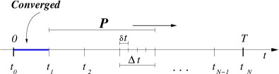
Figure 1: A shifting parallelization window computes $P$ intervals of size $\Delta t$ in parallel. Every interval $\Delta t$ is decomposed in smaller intervals of size $\delta t$

We select an explicit symmetric symplectic integrator $F$, for instance, the leapfrog or any of the $\mathcal{SABA}_{n}$ or $\mathcal{SBAB}_{n}$ integrators [19]. We concatenate $j>1$ schemes to be compute in parallel by each thread. We define $\delta t$ to be the time step of a single $F$ scheme and $\Delta t=j\cdot\delta t$ the interval computed in parallel.

Finally, we open a shifting parallelization window which contains $P$ intervals of size $\Delta t$. $P$ is the number of threads or, if each thread runs on a single processor, $P$ becomes the number of processors in the parallel machine. After each iteration, we verify how many $\Delta t$ intervals have converged and we shift the window until the first non converged $\Delta t$ interval (see Figure 1).

We denote by

$$\mathfrak{F}\left(y_{n+\frac{i}{j}}^{(k)}\right) = c_{i}\cdot\delta t\cdot f_{q}\left(y_{n+\frac{i}{j}}^{(k)}\right)$$

the $i$-th numerical value for the integrable part and by

$$\mathfrak{G}\left(y_{n+\frac{i}{j}}^{(k)}\right) = d_{i}\cdot\delta t\cdot g\left(y_{n+\frac{i}{j}}^{(k)}\right)$$

the corresponding $i$-th value for the perturbing part of the Hamiltonian function. The coefficients $c_{i}$ and $d_{i}$, $i=1,\dots,j$ are selected based on the symplectic underlying integrator.

We show the general structure of the algorithm in the following frame

Algorithm 1. Jiménez-Laskar.

Setup of the initial guess sequence

$y_{0}^{0}=y(0)$, $y_{n+1}^{0}=\mathfrak{F}\left(y_{n}^{0}\right)$

$G_{n}^{0}=0$

While $r<N$ do

Parallel resolution on $[T^{n},T^{n+1}]$ for $r\leq n<r+P$:

For i=1 to j

compute $\mathfrak{F}\left(y_{n+\frac{i}{j}}^{(k)}\right)+\epsilon\mathfrak{G}\left(y_{n+\frac{i}{j}}^{(k)}\right)$,

save $\mathfrak{G}\left(y_{n+\frac{i}{j}}^{(k)}\right)$,

End (For i),

$u_{r+1}=y_{r+1}^{(k)}$

$conv=1.$

Converged=TRUE.

Head=TRUE.

Sequential corrections:

For $n=(r+1)$ to $(r+P)$

For i=1 to j

compute $y_{n+1}^{(k+\frac{1}{2})}=\mathfrak{F}\left(y^{(k+\frac{1}{2})}_{n+\frac{i}{j}}\right)+\epsilon\mathfrak{G}\left(y^{(k)}_{n+\frac{i}{j}}\right)$.

End (For i)

compute $G_{n+1}^{(k+\frac{1}{2})}=\mathfrak{G}\left(y_{n+1}^{(k+\frac{1}{2})}\right)$

compute $y_{n+1}^{(k+1)}=y_{n+1}^{(k+\frac{1}{2})}+\epsilon\left(G_{n+1}^{(k+\frac{1}{2})}-G_{n+1}^{(k-\frac{1}{2})}\right)$.

If Head=TRUE

If Converged=TRUE

$u_{n+1}=y_{n+1}^{(k+1)}$

$conv=conv+1$.

Else

$r=r+conv$ (shifts the window).

Converged=FALSE

Head=FALSE

begins the next parallel iteration

with the available processors.

End (If Converged=TRUE)

End (If Head=TRUE)

End (For n).

End (While).

where the sequence $\{y_{n}^{(k)}\}$ is the $k$-th approximation to the solution $\{u_{n}\}$. It is important to note that this algorithm converges exactly to the sequential underlying integrator.

4 Numerical examples

We have tested our algorithm with the simple Hamiltonian pendulum and the Spin-orbit problem. We have implemented the code in TRIP [14] simulating the parallel implementation for several values of $P$ in order to find $P^{*}$ which optimizes the speed-up function $\mathcal{S}_{P}$. The discussion about this subject will be treated in the next section.

Hamiltonian problems for very long times. In order to reach this, we have tested the algorithm with no tolerance in the error between the sequential solution and the parallel aproximation. It means that we test err==0 at every iteration where err=$\|y_{seq}(t_{n})-y^{(k)}(t_{n})\|$ is the numerical Euclidian distance between the sequential solution $y_{seq}(t_{n})$ and the $k$-th approximation $y^{(k)}(t_{n})$ at time $t_{n}$. Of course, if we relax this condition to the machine tolerance or to the size of the Hamiltonian error at each $\Delta t$ interval we will have a gain in the speed-up function.

Figure 2: The Hamiltonian pendulum. Square of the Euclidean distance between the sequential and the parallel solutions in $\log_{10}$ scale. Each curve corresponds to the $k$-th iteration for $k=10,20,\dots$. The ASD parallel algorithm takes 36 iterations meanwhile the Parareal algorithm takes 109 iterations to total convergence ($err=0$).

4.1 The simple Hamiltonian pendulum

The first example is the simple Hamiltonian pendulum with equation

$$H(p,q) = \frac{1}{2}p^{2}-\epsilon\cos{q}$$ (26)

which we integrate with a $\mathcal{SBAB}_{4}$ symplectic integrator of order $\mathcal{O}(\tau^{8}\epsilon+\tau^{2}\epsilon^{2})$ [19]. We have made several test for different values of $\epsilon$, $\delta t$, $\Delta t$ (in $\delta t$ steps), the size of the simulation $N$ (in $\delta t$ steps) and the size of the shifting parallelization window $P$ ($\Delta t$ intervals in parallel).

Notation 1

We have de following notation:

• $C_{\Delta t}$ will denote the mean number of $\Delta t$ intervals converged to the sequential solution at each iteration.

• $I_{(\tau,P)}$ will denote the mean number of iterations needed to make converge $P$ intervals of size $\Delta t$.

• $k_{(\Delta t,P)}$ will denote the total number of iterations needed to obtain the sequential solution.

These values are related by the following relationships

$$P=C_{\Delta t}\times I_{(\Delta t,P)}\quad{\rm and}\quad k_{(\Delta t,P)}=\frac{N}{jP}I_{(\Delta t,P)}=\frac{N}{jC_{\Delta t}}$$ (27)

where $j\in\mathbb{N}$ is such that $\Delta t=j\delta t$

Table 1 shows values obtained for a simple test with parameters $\epsilon=0.01$, $\delta t=0.01$, $\Delta t=1$, $N=10^{6}$ and the initial conditions $(p_{0},q_{0})=(1,0)$. In this case, we concatenate 100 $\delta t$ steps in a $\Delta t$ interval and the number $P$ of $\Delta t$ intervals computed in parallel varies from 50 to 500 in steps of 50 intervals.

P	$C_{\Delta t}$	$I_{(\Delta t,P)}$	$k_{(\Delta t,P)}$
50	6.9728	7.17072	1434
100	12.018	8.32083	832
150	16.3918	9.15092	610
200	20.5318	9.74097	487
250	24.3285	10.276	411
300	27.6981	10.8311	361
350	30.6718	11.4111	326
400	33.7804	11.8412	296
450	36.36	12.3762	275
500	38.9066	12.8513	257

Table 1. Values obtained for different sizes of the shifting

parallelization window $P$. The values for the parameters are

$\epsilon=0.01$, $\delta t=0.01$, $\Delta t=1$, $N=10^{6}$ and $T=10^{4}$.

We have made several tests for different values in the parameters and we noted that $C_{\Delta t}$, $I_{(\Delta t,P)}$ and $k_{(\Delta t,P)}$ have, in all cases, the same qualitative behavior. In particular, $I_{(\Delta t,P)}$ has an almost linear behavior then we have fitted a straight line $I(P)\sim I_{(\Delta t,P)}$ by least squares technique. Expressions for $C_{\Delta t}$, $I_{(\Delta t,P)}$ and $k_{(\Delta t,P)}$ using (27) are:

$$C_{\Delta t}=\frac{1}{j\left(a+\frac{b}{P}\right)},\quad I_{(\Delta t,P)}=j(aP+b)\quad{\rm and}\quad k_{(\Delta t,P)}=\left(a+\frac{b}{P}\right)N.$$ (28)

Figure 3 shows the data of Table 1 with the fitted curves for the Hamiltonian pendulum with parameters $a=(2.51)^{-4}$ and $b=(7.64)^{-2}$.

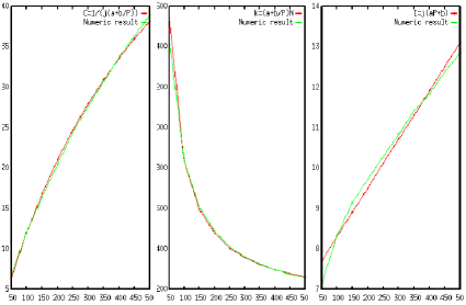
Figure 3: Plots of the data from Table 1 for $C_{\Delta t}$, $I_{(\Delta t,P)}$, and $k_{(\Delta t,P)}$ and its fitting curves with parameters $a=(2.51)^{-4}$ and $b=(7.64)^{-2}$.

4.2 The spin-orbit problem

The next example is the spin-orbit problem with equation

$$H(p,q) = \frac{1}{2}p^{2}-\epsilon\cos{2q}-\alpha(\cos(2q+\phi)-7\cos(2q-\phi))$$ (29)

which we integrate with the same symplectic integrator as in the pendulum case. We have used the parameters $\alpha=10^{-4}$ and $\phi=0.2$ in addition to the values of the last example. Table 2 shows values obtained for a simple test of the spin-orbit problem.

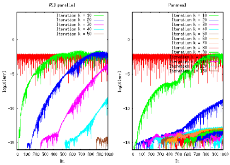
Figure 4: The spin-orbit problem. Square of the Euclidean distance between the sequential and the parallel solutions in $\log_{10}$ scale. Each curve corresponds to the $k$-th iteration for $k=10,20,\dots$. The ASD parallel algorithm takes 54 iterations meanwhile the Parareal algorithm takes 135 iterations to total convergence ($err=0$).

P	$C_{\Delta t}$	$I_{(\Delta t,P)}$	$k_{(\Delta t,P)}$
50	6.08952	8.21082	1642
100	9.81256	10.191	1019
150	12.8028	11.7162	781
200	15.3594	13.0213	651
250	17.6039	14.2014	568
300	19.5293	15.3615	512
350	21.2745	16.4516	470
400	22.9335	17.4417	436
450	23.9211	18.8119	418
500	24.8731	20.102	402

Table 2. Spin-orbit problem: values obtained for different sizes of the

shifting parallelization window $P$. The values for the parameters are

$\epsilon=0.01$, $\alpha=10^{-4}$, $\phi=0.2$, $\delta t=0.01$, $\Delta t=1$, $N=10^{6}$ and $T=10^{4}$.

Figure 5 shows the data of Table 2 with the fitted curves for the spin-orbit problem with parameters $a=(1.19)^{-4}$ and $b=(7.11)^{-2}$.

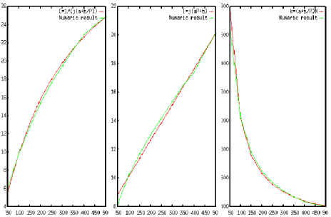
Figure 5: Plots of the data from Table 2 for the spin-orbit problem. We show $C_{\Delta t}$, $I_{(\Delta t,P)}$, and $k_{(\Delta t,P)}$ and its fitting curves with parameters $a=(1.19)^{-4}$ and $b=(7.11)^{-2}$.

4.3 Speed-up of the parallel algorithm

In this subsection we find an expression for the speed-up of the algorithm with parallelization window.

Definition 1

We call speed-up, denoted by $S_{P}(N)$, to the ratio of the time $T_{1}(N)$ required to solve a given problem using the best known serial method to the time $T_{P}(N)$ required to solve the same problem by a parallel algorithm using $P$ processors

$$\mathcal{S}_{N}(P)=\frac{T_{1}(N)}{T_{P}(N)}$$

where $N$ denotes the size of the problem.

We use an alternative notation inverting the parameter $P$ and the variable $N$ since we are interested in finding some expression for the speed-up $\mathcal{S}_{N}(P)$ in terms of $P$. The classical notation is $\mathcal{S}_{P}(N)$.

Let $T_{\mathcal{P}}$ be the predictor’s computing time for a $\Delta t$ interval and let $T_{\mathcal{C}}$ be the corrector’s computing time for the same interval. We suppose we have a first estimation of the solution. Then, the speed-up function for the parallel $\mathcal{SABA}_{n}$ with shifting parallelization window $P$ is given by

$$\mathcal{S}_{N}(P)=\frac{NT_{\mathcal{P}}}{k_{(\Delta t,P)}\left(T_{\mathcal{P}}+PT_{\mathcal{C}}\right)},$$

where $k_{(\Delta t,P)}\in\mathbb{N}$ is the number of iterations to converge. This is the worst case, since with our algorithm we do not wait for ending the $P$ corrections. In fact, a more accurate expression is obtained substituting $P$ by $(P-C_{\Delta t})$. Since, it is desirable to have an expression in terms of $P$ only we use equations (28) to obtain such expression.

In what follows, we assume $k_{(\Delta t,P)}=k(P)$ has an analytic expression equivalent to (28) as in the cases for the Hamiltonian pendule, the spin-orbit problem and the planetary problem (see [18]). After some simplifications and considering $P-C_{\Delta t}$ instead of $P$, the formula for the speed-up becomes

$$\mathcal{S}_{N}(P)=\mathcal{S}(P)=\frac{T_{\mathcal{P}}}{aT_{\mathcal{C}}}\cdot\frac{P}{P^{2}+BP+C},$$ (30)

where

$$B=\left(\frac{T_{\mathcal{P}}}{T_{\mathcal{C}}}+\frac{b}{a}-\frac{1}{ja}\right)\quad{\rm and}\quad C=\frac{bT_{\mathcal{P}}}{aT_{\mathcal{C}}}.$$

Expression (30) does not depend on the size of the problem $N$ (see Figure 6).

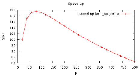
Figure 6: The Speed-up function with parameters $a=(1.19)^{-4}$, $b=(7.11)^{-2}$, $j=100$ and $\frac{T_{\mathcal{P}}}{T_{\mathcal{C}}}=10$.

Since we have a quadratic polynomial in the denominator, we may have vertical asymptotes in its roots. We impose the condition $\mathcal{S}(P)>0$ for $P>0$ which implies $P^{2}+BP+C>0$. Additionaly, we have that $\mathcal{S}(0)=0$, $S(P)>0$ if $P>0$ and since $\lim_{P\to\infty}\mathcal{S}(P)=0$ then there exists a critical point $P^{*}$ which maximize $\mathcal{S}(P)$. We have the following

Proposition 1

If the function $k(P)$ has the form (28), then $\mathcal{S}(P)$ has a maximum in $P^{*}\in\mathbb{N}$ which optimize the parallel algorithm. Moreover, the theoretic optimal speed-up is

$$\mathcal{S}(P^{*})\cong\frac{1}{a+2a\sqrt{\frac{bT_{\mathcal{C}}}{aT_{\mathcal{P}}}}+\left(b-\frac{1}{j}\right)\frac{T_{\mathcal{C}}}{T_{\mathcal{P}}}}$$ (31)

Proof. We consider expression (30) in the extended case $\mathcal{S}:\mathbb{R}\to\mathbb{R}$ and we obtain a differentiable function for $P>0$ such that the original problem is just the restriction $\mathcal{S}|_{\mathbb{N}}$. We procede in the classical way looking for the critical points by differentiation. Since

$$\frac{d\mathcal{S}}{dP}(P) = \frac{T_{\mathcal{P}}}{aT_{\mathcal{C}}}\frac{C-P^{2}}{(P^{2}+BP+C)^{2}},$$

Then the only positive critical (in fact the maximum) point for the extended problem is $P_{*}=+\sqrt{\frac{bT_{\mathcal{P}}}{aT_{\mathcal{C}}}}$. We define

$$P^{*} = \left\{\begin{array}[]{ll}\left[P_{*}\right]&{\rm if}\hskip 20.0pt\mathcal{S}_{N}([P_{*}])-\mathcal{S}([P_{*}]+1)\leq 0\\ \left[P_{*}\right]+1&\hskip 25.0pt{\rm otherwise}.\end{array}\right.$$

where $[\cdot]$ is the maximum integer function. Finally, for the case where $\mathcal{S}([P_{*}])=\mathcal{S}([P_{*}]+1)$ we know that $[P_{*}]$ is optimal then $P^{*}$ is well defined.

The second affirmation is obtained directly by substituting $P^{*}=\sqrt{\frac{bT_{\mathcal{P}}}{aT_{\mathcal{C}}}}$ directly in (30).

$\hfill\square$

Once we know the optimal value for $P^{*}$ as a function of $\frac{T_{\mathcal{P}}}{T_{\mathcal{C}}}$, we are interested in the gain, the speed-up which we can reach with this strategy of parallelizing windows. We write the speed-up function (31) as a function of the ratio $\frac{T_{\mathcal{P}}}{T_{\mathcal{C}}}$ with parameters $a$, $b$ and $j$ as

$$\mathcal{S}_{opt}(P^{*}) = \frac{1}{a+2\frac{b}{P^{*}}+\left(b-\frac{1}{j}\right)\frac{b}{a(P^{*})^{2}}},$$ (33)

From expression (33) we obtain another useful result

Corollary 1

Let $k_{(\Delta t,P)}$ be the number of iterations needed to convergence for the parallel algorithm where $k_{(\Delta t,P)}$ is as in (28) and the parameters $a$, $b$ and $j$ are fixed for some particular problem. The speed-up of the parallel algorithm is bounded by

$$\mathcal{S}(P)<\frac{1}{a}.$$ (34)

Proof. Take the limit for expression (33) when $P^{*}\to\infty$.

$\hfill\square$

5 Additional discussion

What we gain with this algorithm is the time computation of the perturbing terms. Since we have concatenated 100 $\mathcal{SBAB}_{4}$ schemes, we have called 500 times the perturbing function in each parallel step (5 times in each $\mathcal{SBAB}_{4}$). In the sequential correction we gain in time $500C_{\Delta t}T_{\mathcal{B}}$ where $T_{\mathcal{B}}$ is the time used in the computation of the perturbing term. However, we must call the integrable function $400P$ times in the correction step. It means that this algorithm works in problems where $T_{\mathcal{A}}\ll T_{\mathcal{B}}$ like the spin-orbit problem. This is clear from the optimal value of the shifting window $P^{*}=\sqrt{\frac{aT_{\mathcal{P}}}{bT_{\mathcal{C}}}}$ in expression (33) and the fact that $T_{\mathcal{P}}=j(4T_{\mathcal{A}}+5T_{\mathcal{B}})$ and $T_{\mathcal{C}}=4jT_{\mathcal{A}}+T_{\mathcal{B}}$. We have

$$\frac{T_{\mathcal{P}}}{T_{\mathcal{C}}}=\frac{j(4T_{\mathcal{A}}+5T_{\mathcal{B}})}{4jT_{\mathcal{A}}+T_{\mathcal{B}}}=1+\frac{(5j-1)T_{\mathcal{B}}}{4jT_{\mathcal{A}}+T_{\mathcal{B}}}\sim 1+\frac{T_{\mathcal{B}}}{T_{\mathcal{A}}}.$$

Moreover, the time of one iteration for this algorithm using the $\mathcal{SBAB}_{n}$ scheme as underlying integrator is

$$T_{\mathcal{P}}+(P-C_{\Delta t})T_{\mathcal{C}} = j(4T_{\mathcal{A}}+5T_{\mathcal{B}})+(P-C_{\Delta t})(4jT_{\mathcal{A}}+T_{\mathcal{B}})$$

$$= 4j(P-C_{\Delta t}+1)T_{\mathcal{A}}+(4j+P-C_{\Delta t})T_{\mathcal{B}}$$

where $j$ and $P$ must be selected such that the following conditions are fulfilled:

1. $T_{\mathcal{P}}\cong(P-C_{\Delta t})T_{\mathcal{C}}$, this is important to avoid, at maximum, the dead-time in the threads.

2. $T_{\mathcal{P}}+(P-C_{\Delta t})T_{\mathcal{C}}$ be minimal, in order to obtain a large speed-up.

The reader must note that for large values of $P$ or $j$ the algorithm might not work if $T_{\mathcal{A}}\sim T_{\mathcal{B}}$ are comparable. In those cases we have used an alternative corrector scheme to parallelize the La2010 solution (see [20]), such scheme reduces the time $T_{\mathcal{C}}$ but increases the number of iterations needed to convergence (see [18]). Finally, for higher dimensional Hamiltonian problems as the Solar system dynamics, we find that the value of $j$ is very restricted. Some tests with the La2010 solutions [20] accept only a maximum of $8$ $\mathcal{SABA}_{4}$ schemes concatenated in a $\Delta t$ interval, and for $j>8$ the value of $C_{\Delta t}\equiv 1$ which is a worst case than the sequential solution.

References

- [1] C. Audouze, M. Massot and S. Volz, Symplectic multi-time step parareal algorithms applied to molecular dynamics, hal-00358459, Feb 2009.
- [2] A. Bellen and M. Zennaro, Parallel algorithms for initial-value problems for difference and differential equations, J. of Comp. and Appl. Math. 25: 341-350, 1989.
- [3] G. Bal, Parallelization in time of (stochastic) ordinary differential equations, submitted.
- [4] G. Bal, Symplectic parareal, Lecture Notes in Comp. Sci. and Engin. Vol 60(II): 401-408, 2008.
- [5] G. Bal and Y. Maday, A parareal time discretization for non-linear PDE’s with application to the pricing of an American put, Lecture Notes in Comp. Sci. and Engin. Vol 23:189-202, 2002.
- [6] J. Cortial and C. Farhat, A time-parallel implicit method for accelerating the solutions of nonlinear structural dynamics problems, Int. J. Numer. Meth. Engng. ??.
- [7] J. Cortial and C. Farhat, A time-parallel implicit methodology for the near-real-time solution of systems of linear oscillators, L. Biegler, O. Ghattas, M. Heinkenschloss, D. Keyes, and B. van Bloemen Wanders, eds.Real-Time PDE-Constrained Optimization, Springer, 2006.
- [8] X. Dai, C. Le Bris, F. Legoll and Y. Maday, Symmetric parareal algorithms for Hamiltonian systems, preprint, arXiv:1011.6222, 2010.
- [9] J. Erhel and S. Rault, Algorithme parallèle pour le calcul d’orbites, Technique et science informatiques. Vol 19(5): 649-673, 2000.
- [10] C. Farhat and M. Chandesris, Time decomposed parallel time-integrators I: Theory and feasibility studies for fluid, structure, and fluid-structure applications, Int. J. Numer. Methods Eng. 58(9):1397-1434, 2003.
- [11] T. Fukushima, Picard iteration method, Chebyshev polynomial approximation, and global numerical integration of dynamical motions, The Astronomical Journal, Vol 113(5): 1909-1914, 1997.
- [12] T. Fukushima, Vector integration of dynamical motions by the Picard-Chebyshev method, The Astronomical Journal, Vol 113(6): 2325-2328, 1997.
- [13] T. Fukushima, Parallel/Vector integration methods for dynamical astronomy, Cel. Mech. and Dyn. Astr., 73: 231-241, 1999.
- [14] M. Gastineau and J. Laskar, 2010. TRIP 1.1a10, TRIP Reference manual. IMCCE, Paris Observatory. http://www.imcce.fr/trip/.
- [15] M. Gander and E. Hairer, Nonlinear convergence analysis for the parareal algorithm,
- [16] M. Gander and S. Vandewalle, On the superlinear and linear convergence of the parareal algorithm, Lecture Notes in Comp. Sci. and Engin. Vol 55:291-298, 2007.
- [17] A. Griewank, On automatic differentiation, M. Iri and K. Tanabe, eds. Mathematical Programming: Recent Developments and Applications. Kluwer Acad. Pub. 83-108, 1989.
- [18] H. Jiménez-Pérez and J. Laskar The parallel ASD algorithm for Solar system dynamics, preprint, 2011.
- [19] J. Laskar and P. Robutel High order symplectic integrators for perturbed Hamiltonian systems, Celestial Mechanics and Dynamical Astronomy 80(1): 39-62, 2001.
- [20] J. Laskar, A. Frienga, M. Gastineau, H. Manche, La2010: A new orbital solution for the long term motion of the Earth, Astronomy & Astrophysics, in press.
- [21] E. Lelarasmee, A. Ruehli and A. Sangiovanni-Vincentelli, The Waveform relaxation method for time-domain analysis of large scale integrated circuits, IEEE Trans. on Comp.-Aid. Design of Int. Circ. and Syst. Vol. CAD 1(3): 131-145, 1982.
- [22] J.L. Lions, Y. Maday and G. Turinici, Résolution d’EDP par un schéma en temp “pararéel”, C. R. Acad. Sci. Serie I Analyse numérique (332): 1-6, 2001.
- [23] R.I. McLachlan, Composition methods in the presence of small parameters, BIT 35:258-268, 1995.
- [24] R.I. McLachlan, On the numerical integration of Ordinary Differential Equations by symmetric composition methods, BIT 35:258-268, 1995.
- [25] W.L. Miranker and W. Liniger, Parallel methods for the numerical integration of ordinary differential equations, Math. Comp., 91:303-320, 1967.
- [26] J. Nievergelt, Parallel methods for integrating ordinary differential equations, Commun. ACM, 7(12): 731-733, 1964.
- [27] P. Saha and S. Tremaine, Symplectic integrators for solar systems dynamics, The Astron. Jour. Vol 104(4): 1633-1640, 1992.
- [28] P. Saha and S. Tremaine, Long-term planetary integration with individual time steps, The Astron. Jour. Vol 108(5): 1962-1969, 1994.
- [29] P. Saha, J. Stadel and S. Tremaine, A parallel integration method for solar system dynamics, The Astron. Jour. Vol 114(1): 409-415, 1997.
- [30] G. Staff, The parareal algorithm: A survey of present work, NOTUR, 2003.
- [31] M. Suzuki, Fractal decomposition of exponential operators with applications to many-body theories and Monte Carlo simulations, Physicletters A 146:319-323, 1990.
- [32] H. Yoshida, Construction of higher order symplectic integrators, Physics letters A 150(5,6,7):262-268, 1990.