Total Variation Minimization Based Compressive Wideband Spectrum Sensing for Cognitive Radios

Abstract

Wideband spectrum sensing is a critical component of a functioning cognitive radio system. Its major challenge is the too high sampling rate requirement. Compressive sensing (CS) promises to be able to deal with it. Nearly all the current CS based compressive wideband spectrum sensing methods exploit only the frequency sparsity to perform. Motivated by the achievement of a fast and robust detection of the wideband spectrum change, total variation minimization is incorporated to exploit the temporal and frequency structure information to enhance the sparse level. As a sparser vector is obtained, the spectrum sensing period would be shorten and sensing accuracy would be enhanced. Both theoretical evaluation and numerical experiments can demonstrate the performance improvement.

I Introduction

Windband spectrum sensing is a critical component of a functioning cognitive radio system [1]. To simultaneously grab any available channel for secondary systems while avoiding harmful interference to primary receivers, cognitive radios should be able to sense a wide range of frequencies to find ”blank spaces” in the licensed bands which are not being used by primary users at a particular place and time [2].

There are three ways to perform the wideband spectrum sensing: One approach utilizes a bank of fixed narrowband bandpass filters. But it requires an enormous number of Radio Frequency (RF) components and bandpass filters, which lead to high cost. Besides, the number of the bands is fixed and the filter range is always preset. Thus the filter bank way is not flexible. Another approach use a tunable bandpass filter (BPF). Based on a one-by-one search strategy, a BPF can be employed to search one frequency band at a time. However, this approach results in a significantly long search time [3]. The third one is to implement a wideband circuit using a single RF chain followed by high-speed DSP to process the full range of the available spectrum at once [1]. And the major challenge is the too high sampling rate requirement.

Compressive sensing (CS) promises to be able to deal with the high sampling rate problem [4] [6] [5]. To exploit the frequency sparsity of the received wideband signal, CS is a novel sampling technique that can sample sparse signals with sub-Nyquist rates and performs accurate recovery. The survey shows that the fixed spectrum allocation leads to a low spectrum utilization ratio by the primary radios [7], which is also the reason that cognitive radio can use the ”blank spectrum holes” to settle the spectrum scarcity problem. Furthermore, the low spectrum utilization also says that the wiedeband signal is sparse in a wide range of frequency domain with large probability.

CS has turned out to be an effective method to address the wideband spectrum sensing. A pioneering work was done in [8] [9] [10], where CS is exploited for wideband spectrum sensing and the standard l1 norm minimization is used to estimate the original spectrum. Other different types of implementation structures for compressive wideband spectrum sensing have been proposed in [11] [12] [13] [14] [15]. However, nearly all these methods exploit only the frequency sparsity to perform compressive wideband spectrum sensing.

In this paper, the temporal and frequency structure information is jointly taken to incorporate in the compressive wideband spectrum sensing via total variation minimization technique. In the wide monitoring frequency band, though the nonzero frequencies are sparse globally, yet in some local subbands, the nonzero entries may be distributed densely [7]. Therefore, a differential operation on the power spectrum state vector would result in a sparser one. Besides, It is typically that the spectrum occupancy states change slowly in time [7]. And when the initial spectrum states is obtained, it is not the spectrum state but the change of the spectrum states that controls the cognitive radios to perform the dynamical secondary spectrum access. The gradient operation on the spectrum state vectors at two adjacent detection periods can give the the spectrum state change vector which can give sufficient information to enable dynamical spectrum access. Furthermore, as the primary signal is slow-varying, the spectrum state change vector would be sparser than the spectrum state vector. To achieve the differential operation in the joint temporal and frequency domain, total variation [16], which can be interpreted as the l1 norm of the (appropriately discretized) gradient is minimized here. As the sparser vector is used, the spectrum sensing performance would be enhanced.

In the rest of the paper, section II gives the sparse spectrum signal model; In section III, the previous standard compressive wideband spectrum recovery method is described; section IV develops the total variation minimization based compressive wideband spectrum sensing scheme; Section V briefly compares the performance; In section VI, numerical experiments is taken to demonstrate the performance enhancement of the proposed method; Finally Section VI draws the conclusion.

II Signal Model

Suppose that there exists several primary users within a wide frequency range. The entire frequency band is segmented into non-overlapping subbands. Primary users employ Frequency Division Multiplexing with fixed channelization. The locations of these subbands are assumed to be preset and known. But the corresponding power spectral density (PSD) levels are slowly varying in different spectrum sensing periods.

Different types of implementation structures for random sampling for compressive wideband spectrum sensing have been proposed in [17] [18] [19] [20]. The operation to obtain the random samples is usually called analog-to-information convertor (AIC). Briefly an AIC may be conceptually viewed as an ADC operating at Nyquist rate, followed by compressive sampling. Here the AIC is taken to sample the analog baseband signal x(t). For illustration convenience, we detail the algorithm in discrete setting as it did in [8] [9] [10] [11] [12] [13] [14] [15]. Denote the $N\times 1$ stacked vector at the output of the ADC by

$${\bf{x}}_{t}=\left[{\begin{array}[]{*{20}c}{x_{tN}}&{x_{tN+1}}&\cdots&{x_{\left({t+1}\right)N-1}}\\ \end{array}}\right]^{T},~{}~{}t=0,~{}1,~{}\cdots~{},~{}T-1$$ (1)

where the time window for the ADC is set to be the Nyquist sampling duration to recover the signal without aliasing. The corresponding random samples of AIC is:

$${\bf{y}}_{t}=\left[{\begin{array}[]{*{20}c}{y_{tM}}&{y_{tM+1}}&\cdots&{y_{\left({t+1}\right)M-1}}\\ \end{array}}\right]^{T},~{}~{}t=0,~{}1,~{}\cdots~{},~{}T-1$$ (2)

With the $M\times N$ random measurement matrix ${\bf{\Phi}}$, we can formulate the random sampling as:

$${\bf{y}}_{t}={\bf{\Phi x}}_{t}$$ (3)

As only PSD is needed to be estimated here, the phase information of the samples are not necessary. The PSD vector can be obtained directly from the autocorrelation of the samples. Here the signal is assumed to be zero-mean, wide-sense stationary. The autocorrelation at lag j are $r_{x}(j)=E\left[{x_{n}x_{n-j}^{*}}\right]$ and $r_{y}(j)=E\left[{y_{n}y_{n-j}^{*}}\right]$. The autocorrelation vectors of the Nyquist samples (1) and the compressive samples (2) are

$${\bf{r}}_{x,t}=\left[{\begin{array}[]{*{20}c}0&{r_{x,t}(-N+1)}&\cdots&{r_{x,t}(0)}&\cdots&{r_{x,t}(N-1)}\\ \end{array}}\right]^{T}$$ (4)

and

$${\bf{r}}_{y,t}=\left[{\begin{array}[]{*{20}c}0&{r_{y,t}(-M+1)}&\cdots&{r_{y,t}(0)}&\cdots&{r_{y,t}(M-1)}\\ \end{array}}\right]^{T}$$ (5)

respectively. In practice, estimates of the autocorrelation are obtained by averaging over several signal segments. Here it can be easily get:

$${\bf{R}}_{\bf{y}}=E\left[{{\bf{y}}_{k}{\bf{y}}_{k}^{H}}\right]={\bf{\Phi R}}_{\bf{x}}{\bf{\Phi}}^{H}$$ (6)

where

$$\left[{{\bf{R}}_{\bf{x}}}\right]_{i,j}=r_{x}(i-j)=r_{x}^{*}(j-i)$$ (7)

and

$$\left[{{\bf{R}}_{\bf{y}}}\right]_{i,j}=r_{y}(i-j)=r_{y}^{*}(j-i)$$ (8)

Then the relation between the Nyquist autocorrelation vector (NAV) (4) and the compressive autocorrelation vector (CAV) (5) can be formulated [13] :

$${\bf{r}}_{\bf{y}}={\bf{Ar}}_{\bf{x}}$$ (9)

where

$${\bf{A}}=\left[{\begin{array}[]{*{20}c}{{\bf{\bar{\Phi}\Phi}}_{1}}&{{\bf{\bar{\Phi}\Phi}}_{2}}\\ {{\bf{\Phi\Phi}}_{3}}&{{\bf{\Phi\Phi}}_{4}}\\ \end{array}}\right]$$ (10)

Denoting the (i, j)-th element of ${\bf{\Phi}}_{i,j}$ by $\phi_{i,j}^{*}$. The $M\times N$ matrix has it entry as:

$$\left[{{\bf{\bar{\Phi}}}}\right]_{i,j}=\left\{{\begin{array}[]{*{20}c}0&{i=1,j=1,\cdots,N}\\ {\phi_{M+2-i,j}}&{i\neq 1,j=1,\cdots,N}\\ \end{array}}\right.$$ (11)

And the $N\times N$ matrices ${\bf{\Phi}}_{1}$, ${\bf{\Phi}}_{2}$, ${\bf{\Phi}}_{3}$ and ${\bf{\Phi}}_{4}$ are:

$${\bf{\Phi}}_{1}=hankel\left({\left[{{\bf{0}}_{N\times 1}}\right],\left[{\begin{array}[]{*{20}c}0&{\phi_{1,1}^{*}}&\cdots&{\phi_{1,N-1}^{*}}\\ \end{array}}\right]}\right)$$ (12)

$${\bf{\Phi}}_{2}=hankel\left({\left[{\begin{array}[]{*{20}c}{\phi_{1,1}^{*}}&\cdots&{\phi_{1,N}^{*}}\\ \end{array}}\right],\left[{\begin{array}[]{*{20}c}{\phi_{1,N}^{*}}&{{\bf{0}}_{1\times(N-1)}}\\ \end{array}}\right]}\right)$$ (13)

$${\bf{\Phi}}_{3}=toeplitz\left({\left[{{\bf{0}}_{N\times 1}}\right],\left[{\begin{array}[]{*{20}c}0&{\phi_{1,N}}&\cdots&{\phi_{1,2}}\\ \end{array}}\right]}\right)$$ (14)

$${\bf{\Phi}}_{4}=teoplitz\left({\left[{\begin{array}[]{*{20}c}{\phi_{1,1}}&\cdots&{\phi_{1,N}}\\ \end{array}}\right],\left[{\begin{array}[]{*{20}c}{\phi_{1,1}}&{{\bf{0}}_{1\times(N-1)}}\\ \end{array}}\right]}\right)$$ (15)

where hankel(a, b) is a hankel matrix (i.e., symmetric and constant across the anti-diagonals) whose first column is a and whose last row is b; and toeplitz(a, b) is a toeplitz matrix (i.e., symmetric and constant across the diagonals) whose first column is a and whose first row is b.

To monitor a broad band, high sampling rate is needed. It is often very expensive. Besides, too many sampling measurements inevitably increase the storage space and computational burden for (DSP), while spectrum sensing requires a fast and accurate algorithm. CS provides an alternative to the well-known Shannon sampling theory. CS is a framework performing non-adaptive measurement of the informative part of the signal directly on condition that the signal is sparse. According to the FCC report [7], the allocated spectrum is in a very low utilization ratio. That means the sparsity inherently exists in the wideband spectrum. As $\textbf{x}_{t}$ has a sparse representation in frequency domain:

$${\bf{r}}_{\bf{x}}={\bf{\Psi p}}$$ (16)

where ${\bf{\Psi}}$ is the $2N\times 2N$ inverse discrete Fourier transform (DFT) matrix, and p is the $2N\times 1$ PSD vector. And Most of the entries of p are zero or almost zero. When the number of nonzero elements of p is S ($S\ll N$), the signal is said to be S-sparse.

Here an $M\times N$ random projection matrix ${\bf{\Phi}}={\bf{S}}$ is used to sample signals, i.e. ${\bf{y}}_{t}={\bf{S}}{\bf{x}}_{t}$, where $M<N$ and S is a non-Uniform Subsampling or Random Subsampling matrix which are generated by choosing M separate rows uniformly at random from the unit matrix $\textbf{I}_{N}$. Combining (9) and (16), the measurement samples can be represented as

$${\bf{r}}_{y,t}={\bf{A\Psi p}}_{t}={\bf{Dp}}_{t}$$ (17)

where D is the $2M\times 2N$ dictionary for the compressive sparse representation.

III The Standard Compressive Wideband Spectrum Sensing

CS theory asserts that, if a signal has a sparse representation in a certain space, one can use the random measurement to obtain the samples and reconstruct it with overwhelming probability by optimization on condition that the random measurement matrix satisfies the restricted isometry property (RIP) which is a condition on matrices ${\bf{\Phi}}$ which provides a guarantee on the performance of ${\bf{\Phi}}$ in CS. It can be stated as[5] [4]:

$$\left({1-\delta_{s}}\right)\left\|{\bf{y}}\right\|_{2}^{2}\leq\left\|{{\bf{\Phi y}}}\right\|_{2}^{2}\leq\left({1+\delta_{s}}\right)\left\|{\bf{y}}\right\|_{2}^{2}$$ (18)

or all the S-sparse y. where $\left\|{\bf{y}}\right\|_{2}=\left({\sum\nolimits_{i}{\left|{y_{i}}\right|^{2}}}\right)^{{1\mathord{\left/{\vphantom{12}}\right.\kern-1.2pt}2}}$ is the $\mathscr{C}_{2}$ norm of the vector ${\bf{y}}=\left[{y_{1},y_{2},\cdots,y_{M}}\right]^{T}$. The restricted isometry constant $\delta_{s}\in\left({0,1}\right)$ is defined as the smallest constant for which this property holds for all S-sparse vectors y. There are three kinds of frequently used measurement matrices, and the Random Subsampling matrix S which is chosen here is one of the three.

When the RIP holds, a series of recovering algorithm can reconstruct the sparse signal. One is greedy algorithm, such as matched pursuit (MP) [21], orthogonal matched pursuit (OMP) [22]; another group is convex program, such as basis pursuit (BP) [23] [24], LASSO [25] [26] [27] [28] and Dantzig Selector (DS) [29]. Comparing these algorithms, DS has almost the same performance as LASSO. Both of these groups has the advantages and disadvantages. Briefly it can be summarized that convex program algorithm has a more reconstruction accuracy while greedy algorithm has less computing complex.

To find the unoccupied spectrum for the secondary access, the signal in the monitoring band is down-converted to baseband and sampling the resulting analogue signal through an AIC that produces samples at a rate below the Nyquist rate. Afterwards, the autocorrelation of the samples is acquired.

Now the PSD of y(t) is estimated from the autocorrelation. With the random measurement matrix ${\bf{\Phi}}={\bf{S}}$ and the random measurement vector ${\bf{y}}_{t}$ $t=0,~{}1,~{}\cdots~{},~{}T$ , the dictionary D can be the autocorrelation ${\bf{r}}_{y,t}$ and the CWSS can be formulated as

$$\begin{array}[]{c}{\bf{p}}=\mathop{\arg\min}\limits_{\bf{p}}\left\|{\bf{p}}\right\|_{0}\\ {\rm{s}}{\rm{.t}}{\rm{.}}{\bf{y}}_{t}={\bf{Dp}}\\ \end{array}$$ (19)

where $\left\|{\bf{p}}\right\|_{0}$ is the $\mathscr{C}_{0}$ norm which counts the number of nonzero entries of the vector p. The minimization of the $\mathscr{C}_{0}$ norm is the best candidate to encourage the sparse distribution. However, it is not a convex function and the formulated CWSS (19) is not a convex programming.

To convert the CWSS model to a convex programming, the $\mathscr{C}_{0}$ norm is relaxing to the $\mathscr{C}_{1}$ norm. Further more, to enhance the noise suppression performance, LASSO is taken to do the CWSS. It is a shrinkage and selection method for linear regression. It minimizes the usual sum of squared errors, with a bound on the sum of the absolute values of the coefficients. To get more accuracy, we can reformulate the CWSS based on LASSO as

$$\begin{array}[]{c}{\bf{p}}_{LASSO}=\mathop{\arg\min}\limits_{\bf{p}}\left\|{\bf{p}}\right\|_{1}\\ {\rm{s}}{\rm{.t}}{\rm{.}}\left\|{{\bf{y}}_{t}-{\bf{Dp}}}\right\|_{2}\leq\mu\\ \end{array}$$ (20)

where $\mu$ is a parameter bounding the amount of noise in the data, and $\left\|{\bf{p}}\right\|_{1}=\sum\nolimits_{i}{\left|{p_{i}}\right|}$ is the $\mathscr{C}_{1}$ norm of the vector ${\bf{p}}=\left[{p_{(}1),p_{(}2),\cdots,p_{(}2N)}\right]^{T}$. This problem is a second order cone program (SOCP) and can therefore be solved efficiently using standard software packages. It finds the smallest $\mathscr{C}_{1}$ norm of coefficients among all the decompositions that the signal is decomposed into a superposition of dictionary elements. It is a decomposition principle based on a true global optimization. A number of convex optimization software, such as cvx [30], SeDuMi [31] and Yalmip [32] can be used to solve the problem.

IV The Proposed Compressive Wideband Spectrum Sensing

The standard sparse recovery method based CWSS only exploits the sparsity in frequency domain. To further enhance the sensing performance, other structure information can be incorporated. One is that the nonzero frequencies are in clusters [8], and the PSD level in every cluster is almost similar. The differential of the PSD sequence would result in a sparser sequence with most of the nonzero elements locating at the band boundaries. The other structure information is that the similarity of two PSD vectors in adjacent sensing periods is very high as the primary signal is often slow-varying. The differential of the adjacent PSD vector would also result in a sparser vector than the original PSD vectors.

To integrate the differential operations in both temporal and frequency domain, the total variation, which can be interpreted as the $\mathscr{C}_{1}$ norm of the gradient, can be minimized. In CS, the number of measurements required to successfully recover signal is in proportion to the sparsity degree [6]. Hence, the differential operation can reduce the number of measurements required, especially when there are wideband signals in the sensing range. Combining sparsity of PSD and differential PSD, we can obtain an total variation minimization (TVM) based CWSS.

IV-A The TVM Based Compressive Wideband Spectrum Sensing

Assume for each spectrum sensing period, there are T measurement vectors. After the autocorrelation operation, we formulate them into a matrix and get that:

$$\ {\bf{R}}_{2M\times T}=\left[{\begin{array}[]{*{20}c}{{\bf{r}}_{y,1}}&{{\bf{r}}_{y,2}}&\cdots&{{\bf{r}}_{y,T}}\\ \end{array}}\right]$$ (21)

$$\ {\bf{P}}_{2N\times T}=\left[{\begin{array}[]{*{20}c}{{\bf{p}}_{t,1}}&{{\bf{p}}_{t,2}}&\cdots&{{\bf{p}}_{t,T}}\\ \end{array}}\right]$$ (22)

Thus we can reformulate (17) in matrix as:

$$\ {\bf{R}}_{2M\times T}={\bf{D}}_{2M\times 2N}{\bf{P}}_{2N\times T}$$ (23)

Then we can let:

$$\ {\bf{\bar{r}}}_{2TM\times 1}={\mathop{\rm vec}\nolimits}\left({{\bf{R}}_{2M\times T}}\right)$$ (24)

$$\ {\bf{\bar{p}}}_{2TN\times 1}={\mathop{\rm vec}\nolimits}\left({{\bf{P}}_{2N\times T}}\right)$$ (25)

$$\ {\bf{B}}_{2TM\times 2TN}={\bf{D}}_{2M\times 2N}\otimes{\bf{I}}_{T\times T}$$ (26)

Thus we can get:

$$\ {\bf{\bar{r}}}_{2TM\times 1}={\bf{B}}_{2TM\times 2TN}{\bf{\bar{p}}}_{2TN\times 1}$$ (27)

The total variation can be regarded as 2-dimensional differential as:

$$\ {\bf{PV}}=\sum\limits_{i,j}{\left(\begin{array}[]{l}\left|{P(i,j)-P(i-1,j)}\right|+\left|{P(i,j)-P(i,j-1)}\right|\\ +\left|{P(i,j)-P(i+1,j)}\right|+\left|{P(i,j)-P(i,j+1)}\right|\\ \end{array}\right)}$$ (28)

Here the PV can be reformulated as:

$$\ {\bf{PV}}=\left\|{{\bf{V}}_{8TN\times 2TN}{\bf{\bar{p}}}_{2TN\times 1}}\right\|_{1}$$ (29)

where

$$\ {\bf{V}}_{8TN\times 2TN}=\left[{\begin{array}[]{*{20}c}{\left({{\bf{V}}_{1}}\right)_{2TN\times 2TN}}\\ {\left({{\bf{V}}_{2}}\right)_{2TN\times 2TN}}\\ {\left({{\bf{V}}_{3}}\right)_{2TN\times 2TN}}\\ {\left({{\bf{V}}_{4}}\right)_{2TN\times 2TN}}\\ \end{array}}\right]$$ (30)

$$\ {\bf{V}}_{1}=\left[{\begin{array}[]{*{20}c}1&0&0&0&\cdots&0&0&0&0\\ {-1}&1&0&0&\cdots&0&0&0&0\\ 0&{-1}&1&0&\cdots&0&0&0&0\\ \vdots&\vdots&\vdots&\vdots&\ddots&\vdots&\vdots&\vdots&\vdots\\ 0&0&0&0&\cdots&0&{-1}&1&0\\ 0&0&0&0&\cdots&0&0&{-1}&1\\ \end{array}}\right]$$ (31)

$$\ {\bf{V}}_{2}=\left[{\begin{array}[]{*{20}c}{-1_{1,1}}&0&\cdots&{1_{1,2N+1}}&0&\cdots&0\\ 0&{-1_{2,2}}&\cdots&0&{1_{2,2N+2}}&\cdots&0\\ \vdots&\vdots&\ddots&\vdots&\vdots&\ddots&\vdots\\ 0&0&\cdots&{-1_{2TN,2N+1}}&0&\cdots&1\\ \end{array}}\right]$$ (32)

$$\ {\bf{V}}_{3}=\left[{\begin{array}[]{*{20}c}1&{-1}&0&0&\cdots&0&0&0&0\\ 0&{-1}&1&0&\cdots&0&0&0&0\\ \vdots&\vdots&\vdots&\vdots&\ddots&\vdots&\vdots&\vdots&\vdots\\ 0&0&0&0&\cdots&0&1&{-1}&0\\ 0&0&0&0&\cdots&0&0&1&{-1}\\ 0&0&0&0&\cdots&0&0&0&1\\ \end{array}}\right]$$ (33)

$$\ {\bf{V}}_{4}=\left[{\begin{array}[]{*{20}c}{1_{1,1}}&0&\cdots&{-1_{1,2N+1}}&0&\cdots&0\\ 0&{1_{2,2}}&\cdots&0&{-1_{2,2N+2}}&\cdots&0\\ \vdots&\vdots&\ddots&\vdots&\vdots&\ddots&\vdots\\ 0&0&\cdots&{1_{1,2N+1}}&0&\cdots&{-1_{2TN,2TN}}\\ \end{array}}\right]$$ (34)

Based on the above TVM formulation, the CWSS can be formulated as:

$$\ \begin{array}[]{c}{\bf{\bar{p}}}_{TVM1}=\mathop{\arg\min}\limits_{{\bf{\bar{p}}}}\left\|{{\bf{V\bar{p}}}}\right\|_{1}\\ {\rm{s}}{\rm{.t}}{\rm{.}}\left\|{{\bf{Y}}-{\bf{BP}}}\right\|_{2}\leq\mu\\ {\bf{\bar{p}}}={\mathop{\rm vec}\nolimits}\left({\bf{P}}\right)\\ \end{array}$$ (35)

In TVM based CWSS (TVM-CWSS) (35), a more sparser vector is estimated. Thus the sensing performance would be enhanced.

There are T segments of measurement vectors in a sensing period. However, when there are only one measurement vector at current time, the TVM can exploit the sparsity in the differential between the estimated PSD vector and the last time’s PSD. Accordingly, with T = 2, the TVM-CWSS (35) would give the estimated wideband spectrum at current time.

From multiple estimated PSD vectors, the spectrum holes can be located. Also the starting time for of primary radios’ vacancy can be noticed. Experience tells us that for longer time that the spectrum has been in vacancy, the spectrum would be more likely to be unused.

IV-B Performance Evaluation

To Compare the TVM-CWSS and LASSO-CWSS, the required number for successful recovery of the sparse signal is analyzed briefly. We assume that there is no measurement noise or perturbation and let n = 2N. With overwhelming probability, a single piece of PSD vector can be successfully recovered for the convex programming for sparse signal recovery on condition that [6]:

$$\ m\geq CS\log\left({{n\mathord{\left/{\vphantom{nS}}\right.\kern-1.2pt}S}}\right)$$ (36)

where C is some constant.

Suppose that the number of nonzero entries in each column of the estimated PSD matrix R is S. Thus the total number of measurement for successful LASSO-CWSS (20) would be:

$$\ m_{BP}\geq TCS\log\left({{n\mathord{\left/{\vphantom{nS}}\right.\kern-1.2pt}S}}\right)$$ (37)

To analyze the performance of TVM-CWSS (35),we assume that for each the average cluster size is d, and the number of clusters in a single PSD vector is K ($K\ll S$). Thus we have S = Kd. For a single PSD vector recovery, the TVM-CWSS reduce the number of nonzero entries in the estimated sparse vector to be 2K. Therefore, the number of measurement for a vector recovery via TVM would be:

$$\ m\geq KC\log\left({{n\mathord{\left/{\vphantom{n{\left({2K}\right)}}}\right.\kern-1.2pt}{\left({2K}\right)}}}\right)$$ (38)

Besides, As a slow-varying signal, only a small part of the positions of the nonzero entries would changed. The variation includes both the newly emerging nonzero entries and the disappeared entries. Here we assume the number of variation in nonzero elements’ positions is $\Delta$ ($\Delta\ll S$). Apart from the first recovery of the first column when t = 0, the required measurement number for each PSD column recovery is:

$$\ m\geq\Delta C\log\left({{n\mathord{\left/{\vphantom{n{\left(\Delta\right)}}}\right.\kern-1.2pt}{\left(\Delta\right)}}}\right)$$ (39)

Thus, the total number of measurement for successful TVM-CWSS (35) would be:

$$\ m_{TVM}\geq C\left({\left({T-1}\right)\Delta\log\left({{n\mathord{\left/{\vphantom{n{\left(\Delta\right)}}}\right.\kern-1.2pt}{\left(\Delta\right)}}}\right)+K\log\left({{n\mathord{\left/{\vphantom{n{\left({2K}\right)}}}\right.\kern-1.2pt}{\left({2K}\right)}}}\right)}\right)$$ (40)

As $\Delta\ll S$ and $K\ll S$, the minimum number of measurements for successful TVM-CWSS would be much less than LASSO-CWSS’.

V Simulation Results

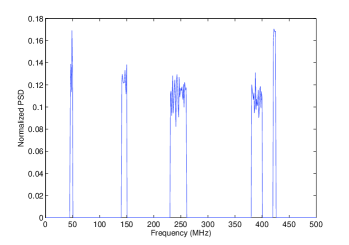
Numerical experiments are presented to illustrate performance of the proposed TVM-CWSS for cognitive radio. Here we consider the initial primary base band signal with its frequency range from 0Hz to 500MHz as Fig. 1 shows. The primary signal with random phase are contaminated by a zero-mean additive Gaussian white noise (AGWN) which makes the signal noise ratio (SNR) be 10dB. Five active block dense bands are randomly located at eight subbands 46MHz - 50MHz, 56MHz - 60MHz, 141MHz - 150MHz, 161MHz - 170MHz, 231-260MHz, 381MHz - 400MHz, 421MHz-425MHz, and 441MHz - 445MHz. The obtained wideband signal has about 14.0$\%$ nonzero entries, which is consistent to the result of practical surveys. Normalizing the energy of the active bands in the wideband, One example of the PSD levels can be given out as Fig. 1 shows. Here we take the noisy signal as the received signal x(t). As CS theory suggests, we sample x(t) randomly at the sub-Nyquist sampling rate via AIC. The resulted sub-sample vector is denoted as $\textbf{y}_{t}$. Here only one measurement vector are available at current time, and the TVM-CWSS exploits the sparsity in the differential between the estimated PSD vector and the last time s PSD.

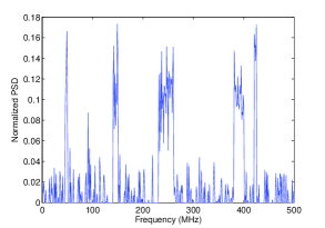
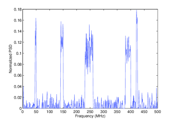
To make contrast, with the same number of samples and fixed nonzero entries in the signal model, power spectrum with different methods with 1000 tries averaged are given out in Fig. 2 and Fig. 3. The compressive measurement is obtained at $0.25\%$ of the Nyquist rate. The parameter $\mu$ is chosen to be $0.05\left\|{{\bf{y}}_{t}}\right\|_{2}$. They show that the proposed TVM-CWSS gives better reconstruction performance. To make details, it shows that there are too many fake spectrum points in the subbands without active primary signals presented in Fig 2 for the standard LASSO. The noise levels of result from LASSO-CWSS are quite high along the whole monitoring band; and the real active frequencies can hardly distinguish themselves. However, in Fig. 3, the active frequencies clearly show up; the noise levels in the inactive bands are quite low. Besides, at other sub-sampling rate, the proposed TVM-CWSS also outperforms the standard LASSO-CWSS in the same way for wideband spectrum sensing. It demonstrates that exploiting the differential frequency sparsity enhances the sensing performance.

To further evaluate the performance, Monte Carlo simulations are used to test the performance. The false alarm ratio vector can be defined as:

$${\bf{p}}_{F}=\left[{\begin{array}[]{*{20}c}{p_{F,1}}&{p_{F,2}}&\cdots&{p_{F,Q}}\\ \end{array}}\right]^{T}$$ (41)

where Q is number of the divided subbands, and for the q-th subband,

$$p_{F,q}=\frac{{TM\left({H_{1,q}|H_{0,q}}\right)}}{L}$$ (42)

where L is the times of Monte Carlo Simulations and ${TM\left({H_{1,q}|H_{0,q}}\right)}$ counts the times when the q-th subband is in vain but the estimation gives the result that it is occupied by primary radio. Similarly, the detection ratio vector can be defined as:

$$\ {\bf{p}}_{D}=\left[{\begin{array}[]{*{20}c}{p_{D,1}}&{p_{D,2}}&\cdots&{p_{D,Q}}\\ \end{array}}\right]^{T}$$ (43)

where for the q-th subband,

$$p_{D,q}=\frac{{TM\left({H_{1,q}|H_{1,q}}\right)}}{L}$$ (44)

where ${TM\left({H_{1,q}|H_{1,q}}\right)}$ counts the times when the estimation correctly gives the result that the q-th sbuband is occupied by primary radio.

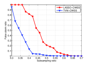
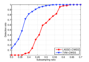
For everyone of the L=1000 simuluations, five subbands are randomly chosen from the eight ones to be active as it shows before. Fig. 4 illustrates the false alarm performance of the 5-th subband (150MHz - 230MHz) via the measurement number for these two CWSS, where the false alarm holds when at least one of the elements in the 5-th subband is larger than one of the elements in the active bands. And Fig. 5 shows the detection ratio performance of the 6-th subband (231MHz - 260MHz) via the measurement number, where the detection holds when all elements in 6-th subband are larger than all of the elements in the inactive bands. The sub-sampling percentage to the Nyquist sampling is from 0.2 to 0.8. Obviously we can see the TVM-CWSS (35) has a remarkable performance gain against LASSO-CWSS (20) for both the false alarm ratio and detection ratio performance.

VI Conclusion

This paper addresses the wideband spectrum sensing for cognitive radio. Because the wideband primary signal often has the nonzero frequencies in cluster, the frequency differential would result in a sparser vector; and because the primary signal is often slow-varying, the differential of the PSD vectors in adjacent sensing period would also give out a sparser vector. Here the total variation minimization is used to perform the joint temporal-frequency differential for compressive wideband spectrum sensing. Both performance analysis and stimulations demonstrate that the TVM-CWSS has performance enhancement.

Figure 1: The normalized spectrum of noiseless active primary signals in the monitoring band.

Figure 2: The normalized estimated spectrum via LASSO-CWSS in the monitoring band.

Figure 3: The normalized estimated spectrum via TVM-CWSS in the monitoring band.

Figure 4: The false alarm performance in the 5-th subband (150MHz - 230MHz) with different sub-sampling rate.

Figure 5: The correct detection performance in the 6-th subband (231MHz - 260MHz) with different sub-sampling rate.

References

- [1] A. Sahai, D. Cabric, ”Spectrum Sensing - Fundamental Limits and Practical Challenges,” A tutorial presented at IEEE DySpan Conference 2005, Baltimore, Nov. 2005.
- [2] S. Haykin, ”Cognitive radio: Brain-empowered wireless communications,” IEEE Journal on Selected Areas in Communications, Vol. 23, No. 2, pp. 201 C220, Feb. 2005.
- [3] A. Ghasemi and E. S. Sousa,”Spectrum sensing in cognitive radio networks: requirements, challenges and design trade-offs,” IEEE Communications Magazine, Vol. 46, No.4, pp. 32 - 39, April 2008.
- [4] D. Donoho, ”Compressed sensing,” IEEE Transactions on information Theory, vol. 52, no. 4, pp. 1289-1306, 2006.
- [5] E. J. Candes, J. Romberg, and T. Tao, ”Robust uncertainty principles: Exact signal reconstruction from highly incomplete frequency information,” IEEE Transactions on Information Theory, vol. 52, no. 2, pp. 489-509, Feb. 2006.
- [6] E. J. Candes; M.B. Wakin ”An Introduction To Compressive Sampling,” IEEE Signal Processing Magazine, Volume 25, Issue 2, pp. 21-30, March 2008
- [7] FCC, Spectrum Policy Task Force Report.ET Docket No. 02-155, Nov. 02, 2002.
- [8] Z. Tian, G. B. Giannakis, ”Compressed Sensing for Wideband Cognitive Radios,” International Conference on Acoustics, Speech, and Signal Processing 2007, Vol. 4, 15-20, April 2007, pp.IV-1357-IV-1360
- [9] Z. Tian, ”Compressed Wideband Sensing in Cooperative Cognitive Radio Networks,” Proceedings of IEEE Globecom Conference 2008, New Orleans , Dec. 2008, pp: 1-5
- [10] Z. Tian, E. Blasch, W. Li, G. Chen, and X. Li, ”Performance Evaluation of Distributed Compressed Wideband Sensing for Cognitive Radio Networks,” Proceedings of the ISIF/IEEE International Conference on Information Fusion (FUSION), Cologne, Germany, July 2008, pp. 1-8
- [11] Jens P. Elsner, Martin Braun, Holger Jakel and Friedrich K. Jondral, ”Compressed Spectrum Estimation for Cognitive Radios,” Proceedings of 19th Virginia Tech Symposium on Wireless Communications, Blacksburg, June 2009, pp: 1-4
- [12] Ying Wang, Ashish Pandharipande, Yvan Lamelas Polo and Geert Leus, ”Distributed Compressive Wide-Band Spectrum Sensing,” IEEE Proceedings of Information Theory Application (ITA’ 09), San Diego (CA), February 2009, pp. 1-4
- [13] Yvan Lamelas Polo, Ying Wang, Ashish Pandharipande, Geert Leus, ”Compressive wideband spectrum sensing, ” International Conference on Acoustics, Speech, and Signal Processing 2009 (ICASSP 2009), Vol. 00, pp. 2337-2340
- [14] Yipeng Liu and Qun Wan ”Robust Compressive Wideband Spectrum Sensing with Sampling Distortion,” CoRR:abs/1005.1803, 2010 [online] accessible at: http://arxiv.org/abs/1005.1803
- [15] Yipeng Liu and Qun Wan, ”Compressive Wideband Spectrum Sensing for Fixed Frequency Spectrum Allocation,” CoRR abs/1005.1804, 2010 [online] accessible at: http://arxiv.org/abs/1005.1804
- [16] Justin Romberg, ”Imaging via compressive sampling [introduction to compressive sampling and recovery via convex programming],” IEEE Signal ProcessING Magazine, Vol. 25, pp. 14 C20, 2008.
- [17] J. N. Laska, S. Kirolos, Y. Massoud, R. Baraniuk, A. Gilbert, M. Iwen, and M. Strauss, ”Random Sampling for Analog-To-Information Conversion of Wideband Signals,” IEEE Dallas Circuits and Systems Workshop (DCAS) 2006, pp: 119-122
- [18] J. N. Laska, S. Kirolos, M. F. Duarte, T. S. Ragheb, R. G. Baraniuk, and Y. Messoud, ”Theory and Implementation of an Analog-To-Information Converter using Random Demodulation,” IEEE Internatianal Symposium on Circuits and Systems (ISCAS) 2007, pp. 1959-1962
- [19] Z. Yu, S. Hoyos, and B. M. Sadler, ”Mixed-signal parallel compressed sensing and reception for cognitive radio,” IEEE International Conference on Acoustics, Speech, and Signal Processing 2008 (ICASSP 2008), March 30 - April 4, 2008, Las Vegas, Nevada, U.S.A, pp. 3861 C3864.
- [20] M. Mishali and Y. C. Eldar, ”Xampling. Part I: Practice,” CCIT Report no. 747, EE Dept., Technion - Israel Institute of Technology, Oct. 2009. [online] accessible at: http://arxiv.org/abs/0911.0519
- [21] Mallat and Z. Zhang, ”Matching pursuit in a time-frequency dictionary,” IEEE Transactions on Signal Processing, vol. 41, pp. 3397 C3415. 1993
- [22] J. A. Tropp and A. C. Gilbert, ”Signal recovery from random measurements via orthogonal matching pursuit,” IEEE Transactions on Information Theory, Vol. 53, No. 12, pp. 4655-4666, 2007
- [23] Shaobing Scott Chen, ”Basis pursuit,”, Department of Statistics, Ph. D dissertation, Stanford University, November 1995
- [24] S. S. Chen and D. L. Donoho, M. A. Saunders, ”Atomic decomposition by basis pursuit,” SIAM Journal on Scientific Computing, Vol. 20, No. 1, pp. 33 - 61, 1999
- [25] R. Tibshirani, ”Regression shrinkage and selection via the lasso,” Journal of the Royal Statistical Society B, Vol. 58, pp. 267 C288, 1996
- [26] B. Efron, I. Johnstone,T. Hastie and R. Tibshirani, ”Least angle regression,” Annals of Statistics, Volume 32, No. 2, pp. 407-499, 2004
- [27] S.-J. Kim, K. Koh, M. Lustig, S. Boyd, and D. Gorinevsky, ”An Interior-Point Method for Large-Scale l1-Regularized Least Squares,” IEEE Journal on Selected Topics in Signal Processing, Vol. 1, No. 4, pp. 606-617, December 2007
- [28] S.-J. Kim, K. Koh, M. Lustig, S. Boyd, and D. Gorinevsky, ”An Interior-Point Method for Large-Scale l1-Regularized Least Squares,” Proceedings International Conference on Image Processing (ICIP), vol. 3, pp. III-117 - III-120, September 2007.
- [29] Emmanuel Candes, and Terence Tao, ”The Dantzig selector: statistical estimation when p is much larger than n”, Annals of Statistics 2007, Volume 35, Number 6, pp. 2313-2351
- [30] Michael Grant, Stephen Boyd, Yinyu Ye, ”cvx user’ guide for cvx version 1.1,” [online] accessible at: http://www.stanford.edu/ boyd/index.html
- [31] J. Sturm, ”Using sedumi 1.02, a matlab toolbox for optimization over symmetric cones,” Optimization Methods and Software, vol. 11, no. 12, pp. 625-653, 1999.
- [32] J. Lofberg, ”Yalmip: Software for solving convex (and nonconvex) optimization problems,” Proceedings of American Control Conference, Minneapolis, MN, USA, June 2006.
- [33] M. Stojnic. ”Strong thresholds for ?2/?1-optimization in block-sparse compressed sensing,” International Conference on Acoustics, Signal and Speech Processing 2009 (ICASSP2009), April 2009. Volume 00, pp. 3025-3028
- [34] M. Stojnic, F. Parvaresh, and B. Hassibi, ”On the reconstruction of block-sparse signals with an optimal number of measurements,” IEEE Transaction on Signal Processing, Vol. 57, No. 8, pp. 3075-3085, August 2009.