Improving measurements of $H(z)$ and $D_{\rm A}(z)$ by analyzing clustering anisotropies

Abstract

The baryonic acoustic feature in galaxy clustering is a promising tool for constraining the nature of the cosmic acceleration, through measurements of expansion rates $H$ and angular diameter distances $\,D_{\rm A}$. Angle-averaged measurements of clustering yield constraints on the quantity $\,D_{\rm A}^{2}/H$. However, to break the degeneracy between these two parameters one must measure the anisotropic correlation function as a function of both line-of-sight (radial) and transverse separations. Here we investigate how to most effectively to do so, using analytic techniques and mock catalogues. In particular, we examine multipole expansions of the correlation function as well as “clustering wedges” $\xi(\Delta\mu,s)$, where $\mu=s_{||}/s$ and $s_{||}$ is the radial component of separation $\vec{s}$. Both techniques allow strong constraints on $H$ and $\,D_{\rm A}$, as expected. The radial wedges strongly depend on $H$ and the transverse wedges are sensitive to $\,D_{\rm A}$. Analyses around the region of the acoustic peak constrain $H$ $\sim 20\%$ better when using the wedge statistics than when using the monopole-quadrupole combination. However, we show that the hexadecapole allows substantially stronger constraints than the monopole and quadrupole alone, as well as analyzing the full shape of $\xi$. Our findings here demonstrate that wedge statistics provide a practical alternative technique to multipoles, that should be useful to test systematics and will provide comparable or better constraints. Finally, we predict the constraints from galaxy clustering that will be possible with a completed version of the ongoing Baryonic Oscillation Spectroscopic Survey.

1 Introduction

The clustering of matter is a powerful tool to probe the evolution of the Universe. In recent years, the baryonic acoustic feature has been detected in the clustering of galaxies. Originating from pre-recombination plasma waves at redshifts $z>1100$, this feature is strongly detected in the temperature fluctuations of the Cosmic Microwave Background radiation (CMB). Its detection at low redshifts serves as an important confirmation of the cold dark matter (CDM) paradigm, and serves as a link between the late and the early Universe (Peebles & Yu 1970, Meiksin et al. 1999).

The baryonic acoustic feature is also a practical cosmic standard ruler (Eisenstein & Hu 1998, Eisenstein et al. 1998, Eisenstein et al. 1999), because the plasma waves left a distinct imprint at the surface of last scattering ($z_{*}\sim 1100$). In the CMB temperature fluctuations $\Delta T/T$ this sound horizon scale of $\sim 150$ physical kpc corresponds to $\sim 1^{\circ}$ in the sky and is known to an accuracy of $<1.5\%$ ($1\sigma$ level; Komatsu et al. 2009). Hence it can be used as a calibrated scale of the angular diameter distance $\,D_{\rm A}(z_{*})$. By measuring a related signature imprinted in the distribution of matter at late times, one can perform geometrical measurements to determine angular diameter distances $\,D_{\rm A}$ at different $z$, as well as measure expansion rates $H$. The importance of this statistical tool is amplified considering the recent discovery of the acceleration of the expansion of the Universe ($z<1$; Riess et al. 1998, Perlmutter et al. 1999). Although both $\,D_{\rm A}$ and $H$ are important cosmic measurements, measuring $H$ directly at various $z$ puts strong constraints on understanding the nature of the apparent acceleration of the observed Universe, e.g through the so-called “dark energy” equation of state $w$ (Blake & Glazebrook 2003, Seo & Eisenstein 2003, Linder 2003, Glazebrook & Blake 2005).

In the matter distribution, this signature appears as oscillations at $k>0.1\,h\,{\rm Mpc}^{-1}$ in the power-spectrum, $P(k)$, corresponding to a bump of excess overdensity in the two-point correlation function, $\xi(s)$, at the characteristic comoving scale of $\sim 100$  $h^{-1}$Mpc. This scale, although not equal to the sound-horizon, is closely related to it, with well-understood differences (Meiksin et al. 1999, Smith et al. 2008, Crocce & Scoccimarro 2008, Sánchez et al. 2008).

The baryonic feature is imprinted in $\xi(\mu,s)$ and can be used to measure $H$ and $D_{\rm A}$. For purely geometric reasons, radial clustering (i.e, clustering in the line-of-sight of the observer; $\mu=1$) contains $H(z)$ information, where the transverse direction ($\mu=0$) yields $\,D_{\rm A}(z)$, where $\mu$ is the cosine of the angle between the total separation of the galaxies and the radial direction.

For S/N reasons, most studies have focused on the angle averaged signal (monopole) $\xi_{0}(s)$ (Eisenstein et al. 2005, Martinez et al. 2009, Cabré & Gaztañaga 2009, Labini et al. 2009, Sánchez et al. 2009, Kazin et al. 2010a, Beutler et al. (in prep)), $P_{0}(k)$, (Cole et al. 2005, Tegmark et al. 2006, Hütsi 2006, Percival et al. 2007, Percival et al. 2010, Reid et al. 2010, Blake et al. 2011) and wavelets (Arnalte-Mur et al. 2011) in clustering of galaxies and galaxy-clusters of the SDSS (York et al. 2000), the Two Degree Field Galaxy Redshift Survey (Colless et al. 2003), the WiggleZ (Drinkwater et al. 2010) survey and the 6dF Galaxy Survey (Jones et al. 2009) galaxy samples. The feature in the projected two-point function of photo-$z$ samples has been analysed by (Padmanabhan et al. 2007, Blake et al. 2007, Estrada et al. 2009, Crocce et al. 2011).

The  baryonic acoustic feature in the monopole has been shown to constrain the cosmological information in combination $\,D_{\rm A}^{2}/H$. The degeneracy of this combination limits its constraining power on expansion models. In this study we discuss techniques to use anisotropic clustering to break this degeneracy.

Radial clustering measurements have been attempted on the Sloan Digital Sky Survey (SDSS) Luminous Red Galaxy sample (LRGs;  Gaztañaga et al. 2009), as well as on the much smaller volume MAIN sample (Tian et al., 2010). Interestingly, both studies show strong clustering measurements, relative to the monopole and $\Lambda$CDM predictions, near where the baryonic acoustic feature is expected. However, Kazin et al. (2010b) suggested a different interpretation of these measurements indicating that the measurement could be the result of sample variance due to the limited volume.

A few studies have investigated using the information from the full $P(\mu,k)$ plane to constrain dark energy by using geometric redshift distortions. Alcock & Paczynski (1979) describe how an intrinsically spherical system appears anisotropic due to geometric distortions. They point out that by reconstructing the original spherical shape, the true cosmology can be obtained. This effect is manifested in clustering measurements, which are assumed to be isotropic (the cosmic principle). When converting the observed redshifts to comoving distances, the observer is required to assume a fiducial cosmology. Choosing an incorrect cosmology causes geometric redshift-distortions (in addition to the dynamical distortions, due to peculiar velocities of the galaxies). For this reason the observed clustering signal provides an opportunity to apply the Alcock-Paczynski test and constrain the true underlying cosmology, assuming dynamical effects are understood (Kaiser 1987). In practice, the  baryonic acoustic feature plays an important role as it breaks degeneracies between amplitude uncertainties ($\sigma_{8}$, bias of tracer to underlying matter over-densities) and geometric shifts.

Hu & Haiman (2003) suggested disentangling $H$ from $\,D_{\rm A}$ by analyzing baryonic acoustic rings in the two-dimensional power spectrum. Focusing on phase shifts, they found that this technique, based only on geometric effects, can constrain the expansion rate of the Universe when applied to galaxy and galaxy-clusters samples at intermediate redshifts $z<0.5$, combined with CMB priors. Wagner et al. (2008) used mock catalogues at $z=1,3$ to demonstrate the usefulness of the technique, and show that light-cone effects do not have a significant impact on the results. Shoji et al. (2009) argue that $H$ and $\,D_{\rm A}$ information is encoded in the full 2D shape, and present a generic algorithm that attempts to take into account dynamic distortions on all scales, assuming non-linear effects are understood. For a first attempt to use the $\xi(s_{\perp},s_{||})$ plane of the SDSS LRGs to constrain cosmology, see Okumura et al. (2008).

These studies, though, do not take into account the complexity of constructing a realistic, reliable (and invertible) covariance matrix for the full 2D measurement of the power spectrum or correlation function. Also, one short-term concern is the fact that near future surveys will have low S/N in the 2D plane.

Padmanabhan & White (2008) investigated a more practical approach in which the 2D results are projected into one dimensional statistics. They proposed to break the $H-\,D_{\rm A}$ degeneracy by combining  AP analysis of the monopole of the correlation function, $\xi_{0}$, with the quadrupole, $\xi_{2}$. They argue that these measurements can constrain the warping in the 2D correlation function which is sensitive to $\,D_{\rm A}\cdot H$, breaking the $\,D_{\rm A}^{2}/H$ degeneracy obtained when probing dilations in the monopole.

Here we follow up on their analysis by:

1. Investigating the effects of higher order multipoles;

2. Introducing a new alternative projection statistic in the form of clustering wedges;

3. Performing the analysis, for the first time, in configuration space ($\xi(\mu,s)$).

We propose to use wide clustering wedges $\xi(\Delta\mu,s)$ to yield constraints on $H$ and $\,D_{\rm A}$. A similar concept has been suggested by Kazin et al. (2010b) (e.g., see their Figure 7). Tests performed here convincingly show that even a wide “transverse” wedge of $0<\mu<0.5$ strongly depends on $\,D_{\rm A}$ and a wide “radial” wedge of $0.5<\mu<1$ constrains $H$. We show that these $\Delta\mu=1/2$ wedges do have intermixing terms, but these can be corrected for and are reduced with decreasing $\Delta\mu$.

The outline of the paper is as follows: in §2 we describe the statistical methods and the mock galaxy catalogues used in our analysis. In §3 we describe various theoretical aspects of $z-$distortions (§3.1), the implicatoins of the AP effect on basic cosmological parameters via determinations of $H$ and $\,D_{\rm A}$ (§3.2), the different clustering statistics used in our analysis (§3.3), and the extraction of $H$ and $\,D_{\rm A}$ information through the  AP test (§3.4). In §4 we run two proof of concept tests. Using mock catalogues, we show that the geometrically distorted signal can be retrieved from the true signal through the  AP test (§4.1), and by doing so retrieve unbiased constraints on $H$ and $\,D_{\rm A}$. We start with the ideal case in which all effects are known except for the  AP effect in §4.2, and then, in §4.3, we gradually add amplitude effects. In §4.4 we investigate the uncertainties of $H$ and $\,D_{\rm A}$ as a function of the separation range used and compare the results obtained by the various 1D projection combinations. In §5 we present predictions for BOSS. Finally, §6 presents a discussion, and §7 our main conclusions

Unless otherwise stated, we use the standard flat $\Lambda$CDM cosmology ($\Omega_{\rm K}=0$, $w=-1$) with $[\Omega_{\rm M0},\Omega_{b0},h,n_{s},\sigma_{8}]=[0.25,0.04,0.7,1,0.8]$. We test geometric distortions by varying only the equation of state of dark energy $w$, when converting $z$ to comoving distances. Our choices of distortions are explained in §3.2 compared to expected degeneracies for various choices of curvature $\Omega_{\rm K}$, and matter density $\Omega_{\rm M0}$. Unless stated otherwise, all distances hereon are comoving.

To avoid semantic confusion, we briefly explain here the terminology of the different spaces we explore. First, all analyses are based on two-point correlation functions, which we refer to as configuration-space, as opposed to $k-$space. Second, because geometric redshift distortions and dynamic redshift distortions are different in nature, we minimize the use of the generic term for both, “redshift distortions”, and call them “geometric distortions” and “dynamical distortions”. Because we analyse geometric distortions with and without dynamical effects, hereon we avoid using the common expression redshift-space ($z-space$). Instead, when dynamical effects are applied we refer to it as velocity-space, and when they are not we refer to it as real-space.

2 Methods of Analysis

2.1 Statistical tools

In our analyses we use the Landy & Szalay (1993) $\xi$ estimator. For details of usage please see Appendix E.

When constraining parameters, we use the standard $\chi^{2}$ technique, where

$$\chi^{2}(\Phi)=\sum_{i,j}\left(M_{i}\left(\Phi\right)-D_{i}\right)C_{ij}^{-1}(M_{j}(\Phi)-D_{j}),$$ (1)

where $i,j$ are the bins tested. For reasons described below, the “data” $D$ is given by the distorted measurement, $\xi^{\mathcal{D}}$, meaning $\xi$ measured from our mock catalogues when using the incorrect cosmology to convert redshifts to comoving distances (the  AP effect). The base-template used for modelling is $\xi^{\mathcal{T}}$, meaning the actual true clustering signal. Hence, the models $M$ are given by the shifted measurements $\xi^{\mathcal{S}}$, that is the result of using the parameters $\Phi$ to shift the template $\xi^{\mathcal{T}}$.

When limiting $\Phi$ to [$H,\,D_{\rm A}$] we calculate $\chi^{2}$ using brute force on a 2D grid. When investigating a larger parameter space, we apply a Monte-Carlo-Markov-Chain (MCMC). We verify that both methods yield similar results.

The statistics we use have covariant uncertainties. (e.g., see Figure 4 in Taruya et al. 2011 for the correlation coefficient between $\xi_{0}$ and $\xi_{2}$.) For this reason we define $D$ and $M$ in array format. For example, when analyzing monopole, quadrupole ($\ell=0,2$) the data is defined as $D=[\xi_{0},\xi_{2}]=\xi_{[\ell]}$.

We construct the covariance matrix $C_{ij}$ from the $N_{\rm mocks}=160$ mock true signals. (For mock description see §2.2.) When using multipoles (or wedges) combination $\xi_{[\ell]}$, we define the covariance matrix as:

$$C_{ij}=\frac{1}{N_{\rm mocks}}\sum_{m,n=1}^{N_{\rm mocks}}\left((\xi_{[\ell]})_{i}^{m}-(\xi_{[\ell]})_{j}^{n}\right)\left((\xi_{[\ell]})_{j}^{m}-(\xi_{[\ell]})_{i}^{n}\right).$$ (2)

2.2 Mock galaxy catalogs

To simulate the observer’s point of view, we analyse the mock galaxy catalogues from LasDamas and the Horizon Run. A similar version of these mock catalogues has been used in our previous analyses of the monopole (Kazin et al. 2010a) and radial clustering (Kazin et al. 2010b).

The LasDamas simulations use a cosmology of [$\Omega_{M0},\Omega_{b0},n_{s}$,$h$,$\sigma_{8}$]=[0.25,0.04,1,0.7,0.8] and the Horizon Run uses [0.26,0.044,0.96,0.72,0.8], where $\Omega_{b0}$ is the present baryonic density and $n_{s}$ is the spectral index. Both these cosmologies are well motivated by constraints obtained by WMAP 5-year measurements of temperature fluctuations in the cosmic microwave background (Komatsu et al., 2009). To understand effects of velocity-space we analyse all volumes both in velocity- and real-space.

The LasDamas collaboration provides realistic LRG mock catalogues by placing galaxies inside dark matter halos using a Halo Occupation Distribution (HOD; Berlind & Weinberg 2002). HOD parameters were chosen to reproduce the observed number density as well as the projected two-point correlation function $w_{p}(r_{p})$ of galaxies in the SDSS-LRG sample at separations $0.3<r_{p}<30$ $h^{-1}$Mpc, below the scales considered here. For more details see McBride et al. (in prep.). We use a suit of 160 LRG volume-limited mock catalogues constructed from light cone samples with a mean number density of $\bar{n}\sim 10^{-4}\,h^{3}\rm{Mpc}^{-3}$. Each mock catalogue covers the redshift range $0.16<z<0.44$ and reproduces the SDSS angular mask, giving a volume of $1.2\,{\rm Gpc}^{3}h^{-3}$. The LasDamas real-space catalogues are similar to the velocity-space catalogues in all aspects, with the exception of the shift in $z$ due to peculiar velocities.

The Horizon Run provides an ensemble of $32$ BOSS volume realizations of mock LRG samples with a higher number density than DR7, $\bar{n}\sim 3\times 10^{-4}\,h^{3}\rm{Mpc}^{-3}$, as expected in BOSS. LRG positions are determined by identifying physically self-bound dark matter sub-halos that are not tidally disrupted by larger structures. For full details see Kim et al. (2009). We construct these mock catalogues by dividing each of the eight full sky samples of the Horizon Run into four quadrants. We map real-space into velocity-space, and limit the samples to the expected volume-limited region of the BOSS LRGs $(0.16<z<0.6)$.

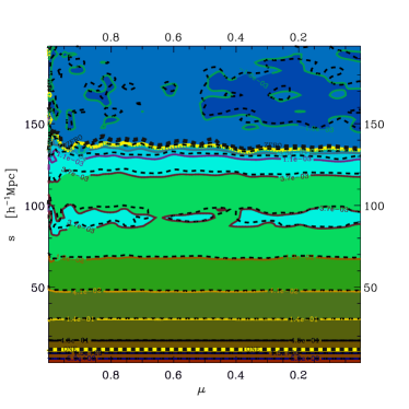
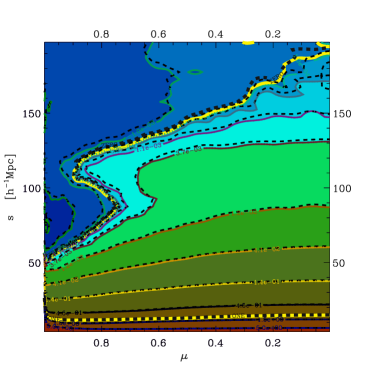
Figure 1: Mean two-dimensional correlation functions $\xi(\mu,s)$ from the ensemble of mock catalogues in real- (left) and velocity-space (right). The contours are spaced logarithmically between 5 and $10^{-4}$ for positive values, and at $-0.001,-0.005,-0.01$ for negative values. The contours corresponding to the values $0,1$ are colored with thick yellow lines. The solid contour lines, following the color scheme, correspond to the result obtained when using the correct cosmology when converting $z$ to comoving distances. The dashed lines show the geometrical distortions obtained by assuming $w^{\mathcal{D}}=-1.1$ instead of the true value $w^{\mathcal{T}}=-1$. It can be clearly seen that dynamical effects dominate over the geometric.

3 Theory

3.1 Redshift distortions: geometric vs. dynamic

Redshift distortions arise due to two effects when converting the redshift $z_{\rm obs}$ of a galaxy into a comoving distance:

$$\chi=c\int_{0}^{z_{\rm obs}}{\frac{dz}{H(z)}}.$$ (3)

The first effect involves the assumption that the observed redshift is produced entirely by the expansion of the Universe $z_{\rm cos}$. This assumption is, of course, incorrect in the presence of peculiar velocities, which introduce an additional Doppler component $z_{\rm pec}$ leading to radial shifts in the infered distances. Although these shifts are small compared to the true distance $\chi(z_{\rm cos})$ (less than $1\%$ at $z\sim 0.3$), they strongly affect clustering measurements which depend on separations between galaxies. We refer to these as dynamical distortions.

Another, more subtle, redshift distortion effect arises due to the conversion of redshift to distance using only approximately known cosmological parameters. The conversion relies on the Hubble parameter (Friedman 1922)

$$H(z)^{2}=H_{0}^{2}\left(\Omega_{\rm M0}\left(1+z\right)^{3}+\Omega_{\rm K}\left(1+z\right)^{2}+\Omega_{\rm{\rm DE}}e^{\int_{0}^{z}{\frac{1+w\left(z^{\prime}\right)}{1+z^{\prime}}dz^{\prime}}}\right),$$ (4)

where $\Omega_{i}$ are the standard cosmological density terms at present day for matter (M0), curvature (K) and dark energy (DE). The Hubble constant $H_{0}\equiv H(0)$ (Hubble & Humason 1931) factors out trivially and we thus express comoving distance in units of  $h^{-1}$Mpc, where $h\equiv H_{0}/(100\,{\rm km}\,{\rm s}^{-1}{\rm Mpc}^{-1}$). The rest of the parameters have more important, and potentially measurable, effects. We refer to these  AP effects as geometric distortions.

One way of overcoming these effects is to recalculate clustering statistics for every set of parameters when determining cosmological constraints. However, that approach is currently not practical. Instead, we calculate $\xi$ using a fixed fiducial set of parameters, and vary the result using linear equations. As we show below, this method is accurate enough.

Figure 1 illustrates dynamic and geometric distortions in the LasDamas mock catalogues using the anisotropic $\xi$ in the $\mu-s$ plane. The information in this coordinate choice is similar to that in the commonly used $s_{||}-s_{\perp}$ plane. We define $\vec{s}$ to be the spatial separation vector with radial and transverse components $s_{||}$, $s_{\perp}$. In real-space (left panel) the true signal corresponds to flat horizontal contour levels in $\xi(\mu,s)$, shown as colored contours (solid lines) A noticeable signature is the  baryonic acoustic feature around $s\sim 110$ $h^{-1}$Mpc.

The dashed lines show the result when we introduce geometric distortions by using $w=-1.1$ instead of the true value $w=-1$ in converting redshifts to comoving distance. These distortions are more noticeable at large scales, though they are also present on small scales.

The right-hand panel illustrates the equivalent measurements with the addition of dynamical distortions (velocity-space). It can be clearly seen that the dynamical distortions dominate over the geometric ones.

Three noticeable features are worth mentioning here. First, the velocity dispersion effect is clearly seen in the clustering signal along the line of sight ($\mu=0$). Although commonly regarded as a small scale effect, it is still present on scales of $60$ $h^{-1}$Mpc, as discussed by Scoccimarro (2004).

Second,the negative sea along the radial direction is apparent at $s\sim 60$ $h^{-1}$Mpc in this cosmology. Notice that in real-space (left plot) $\xi$ turns negative only at $\sim 135$ $h^{-1}$Mpc.

Third, the  baryonic acoustic feature, which appears as a positive stripe in real-space clustering, appears here as ridges which decrease strongly in amplitude towards the line-of-sight. Here the radial baryonic acoustic peak is negative, but can be positive depending on the value of the squashing parameter $\beta\equiv f/b$.

Kaiser (1987) originally describes linear dynamical distortions by coupling the logarithmic rate of change of the growth of structure $f$ to $\mu$. By doing so he related the underlying real-space isotropic $P(k)$ to the apparent anisotropic velocity-space one. The bias $b$ is introduced when relating to matter tracers. In this study we focus on the more subtle geometric distortions, and refer the reader to Hamilton (1998) for a review of dynamical distortions.

3.2 The cosmological power of the  AP effect

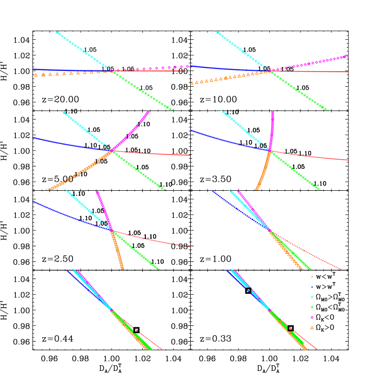
Figure 2: Each panel displays the degeneracies between $\Phi$=[$w$, $\Omega_{\rm M0}$, $\Omega_{\rm K}$] in the $H-\,D_{\rm A}$ plane as a function of $z$. The axes, are in units of a “true” cosmology $\Phi=[-1,\ 0.25,0]$. The “false” values are given in fractions in increments of $\Delta(frac)=0.005$. The legend reads such that: $w<w^{\,{\mathcal{T}}}$ means $w=w^{\,{\mathcal{T}}}\cdot frac$, $w>w^{\,{\mathcal{T}}}$ means $w=w^{\,{\mathcal{T}}}/frac$, $\Omega_{\rm M0}>\Omega_{\rm M0}^{\,{\mathcal{T}}}$ means $\Omega_{\rm M0}=\Omega_{\rm M0}^{\,{\mathcal{T}}}\cdot frac$, $\Omega_{\rm M0}<\Omega_{\rm M0}^{\,{\mathcal{T}}}$ means $\Omega_{\rm M0}=\Omega_{\rm M0}^{\,{\mathcal{T}}}/frac$, $\Omega_{\rm K}>0$ means $frac-1$ and $\Omega_{\rm K}<0$ means $1-frac$. In some high $z$ panels we highlight $5,10\%$ deviations in $\Phi$. The thick boxes at low $z$ indicate the geometric effects we test in this study. The figure clearly shows that at (cosmologically) low redshifts there is a large degeneracy between the parameters. This is relaxed at higher redshifts where distortions in $\Omega_{\rm K}$ and $w$ effect mostly $\,D_{\rm A}$, and distortions in $\Omega_{\rm M0}$ yield similar results to low $z$.

Throughout this study we explore techniques to break the geometric $H-\,D_{\rm A}$ degeneracy with clustering. Here we examine how these constraints are related to fundamental cosmological parameters assuming a $\Lambda$CDM model.

Following Hogg (1999) we define the transverse comoving distance as:

$$D_{\rm M}=\left\{\begin{array}[]{lll}D_{\rm H}\frac{1}{\sqrt{\Omega_{\rm K}}}\sinh\left(\sqrt{\Omega_{\rm K}}\frac{\chi}{D_{\rm H}}\right)&\mbox{for $\Omega_{\rm K}>0$};\\ \chi&\mbox{for $\Omega_{\rm K}=0$};\\ D_{\rm H}\frac{1}{\sqrt{-\Omega_{\rm K}}}\sin\left(\sqrt{-\Omega_{\rm K}}\frac{\chi}{D_{\rm H}}\right)&\mbox{for $\Omega_{\rm K}<0$},\end{array}\right.$$ (5)

where $D_{\rm H}$ is the Hubble distance $c/H_{0}$, and is related to the angular diameter distance by $D_{\rm M}=\,D_{\rm A}(1+z)$. As we explain in §3.4, the  AP effect can be quantified by the dilation and warping parameters $\alpha$ and $\epsilon$, which depend, in turn, on both $H$ and $\,D_{\rm A}$ (see Equations 15, 16). These quantities depend in a non-straightforward fashion on the density parameters $\Omega_{i}$, and the dark energy equation of state $w$. $H$ is given by Equation (4), while $\,D_{\rm A}$ depends on $H$ and $\Omega_{\rm K}$ according to Equations (3) and (5) .

Figure 2 shows how $H$ and $\,D_{\rm A}$ depend on cosmological parameters for a number of redshifts. In each panel (each redshift) we hold two of the three parameters $\Omega_{\rm M0}$, $\Omega_{\rm K}$, and $w$ (where $\Omega_{\Lambda}\equiv 1-\Omega_{\rm M0}-\Omega_{\rm K}$) fixed to a “true” value and modify the third from its fiducial according to the fraction indicated in the legend, between $1$ to $1.5$. We clearly see that at low redshifts $H$ and $\,D_{\rm A}$ yield degenerate constraints on $w$, $\Omega_{\rm K}$ and $\Omega_{\rm M}$ that can be broken as $z$ increases. We notice that the dependence on $\Omega_{\rm M0}$ does not vary much as a function of redshift, where both $\Omega_{\rm K}$ and $w$ align with the $\,D_{\rm A}$ axis at high $z$, meaning $H$ is not sensitive to these parameters.

This plot demonstrates that the $\Omega_{i},\ w$ degeneracy can be broken when applying the  AP effect at high redshift ($z>2$).

In this study we examine  AP effects when varying $w$ at mock mean redshifts $\langle{z}\rangle=0.33$, and 0.44 as indicated by thick boxes in bottom panels of Figure 2. Figure 2 demonstrates that our results are similar to those we would have obtained by choosing to vary $\Omega_{\rm K}$ or $\Omega_{\rm M0}$.

3.3 One-dimensional projections of $\xi(\mu,s)$: introducing clustering wedges

We define clustering wedges as

$$\xi(\Delta\mu,s)\equiv\frac{\int^{\mu_{\rm max}}_{\mu_{\rm min}}{\xi(\mu^{\prime},s)}{{\rm d}\mu^{\prime}}}{\int^{\mu_{\rm max}}_{\mu_{\rm min}}{{\rm d}\mu^{\prime}}},$$ (6)

where $\mu$ is the cosine of the angle between the total separation of the galaxies $\vec{s}$ and the line of sight. We assume here the plane-parallel, or small angle, approximation according to which two galaxies at the same distance from the observer yield $\mu=0$ irrespective of their angular distance. We note that the  baryonic acoustic feature scale at $z=0.3$ corresponds to $\sim 7^{\circ}$ in the sky, and is smaller at larger redshifts. Samushia et al. (2011) discuss observer angle effects. Due to our methods of building templates, our models incorporate large angle effects, and we do not test for them.

Using spherical harmonics, the anisotropic $\xi(\mu,s)$ may be written as:

$$\xi(\mu,s)=\sum_{{\rm even}\ \ell}{\mathcal{P}}_{\ell}(\mu)\xi_{\ell}(s),$$ (7)

where ${\mathcal{P}}_{\ell}$ are Ledgendre polynomials (e.g, ${\mathcal{P}}_{0}=1$, ${\mathcal{P}}_{2}=\frac{1}{2}(\mu^{2}-1)$, ${\mathcal{P}}_{4}=\frac{1}{8}(35\mu^{2}-30\mu+3)$) and

$$\xi_{\ell}\equiv\frac{2\ell+1}{2}\int^{1}_{-1}{\mathcal{P}}_{\ell}(\mu)\xi(\mu,s){\rm d}\mu.$$ (8)

Equations (6) and (7) can be used to find the relation between the clustering wedges and the multipoles. Discarding contributions from multipoles with $\ell>2$ this relation is given by:

$$\xi(\Delta\mu,s)=\xi_{0}+\frac{1}{2}\left(\frac{\mu_{\rm max}^{3}-\mu_{\rm min}^{3}}{\mu_{\rm max}-\mu_{\rm min}}-1\right)\xi_{2}.$$ (9)

A hexadecapole term would mean an additional term given by

$$\frac{1}{8}\left(\frac{7\left(\mu_{\rm max}^{5}-\mu_{\rm min}^{5}\right)-10\left(\mu_{\rm max}^{3}-\mu_{\rm min}^{3}\right)}{\mu_{\rm max}-\mu_{\rm min}}+3\right)\xi_{4}$$ (10)

on the right hand side of Equation (9), and higher multipoles can be calculated in a similar manner.

For simplicity, in this study we focus on clustering wedges defined by a width of $\Delta\mu=1/2$. Of course, this analysis can be generalized to various wedge widths. We discuss the results obtained with various values of $\Delta\mu$ in Appendix B.

Defining the radial wedge $\xi_{||}$ as that given by $0.5<\mu<1$ and the transverse $\xi_{\perp}$ as $0<\mu<0.5$, Equation (9) yields:

$$\left(\begin{array}[]{c}\xi_{||}\\ \xi_{\perp}\end{array}\right)=\left(\begin{array}[]{c c}1&\frac{3}{8}\\ 1&-\frac{3}{8}\end{array}\right)\left(\begin{array}[]{c}\xi_{0}\\ \xi_{2}\end{array}\right),$$ (11)

or

$$\left(\begin{array}[]{c}\xi_{0}\\ \xi_{2}\end{array}\right)=\left(\begin{array}[]{c c}\frac{1}{2}&\frac{1}{2}\\ \frac{4}{3}&-\frac{4}{3}\end{array}\right)\left(\begin{array}[]{c}\xi_{||}\\ \xi_{\perp}\end{array}\right).$$ (12)

The hexadecapole term would add a third column in the matrix on the right side of Equation (11) with absolute values of $15/128\sim 0.12$.

If $\xi(\mu,s)$ consisted only of $\ell=0,2$ terms, the two $\Delta\mu=0.5$ wedges would form a complementary basis to that of the multipoles. In the more generic case, these wide clustering wedges comprise an alternative, but not totally complementary basis. It is easy to see that given any combination of even $\ell$s, the monopole is always the average of the $\Delta\mu=0.5$ wedges, but the quadrupole is combined with higher order multipole terms in a complicated fashion. This means that given non-zero $\xi_{\ell>2}$ terms, these wide wedges do not contain exactly the same information as [$\xi_{0},\xi_{2}$], and hence form an alternative, non-complementary basis. To have a fully complementary basis to $\xi$ which contains $N$ multipoles would, of course, require the same number of wedges (or any other projection).

In Appendix D we test the relationships between the clustering wedges and multipoles. We find that the two wide clustering wedges ($\Delta\mu=0.5$) are defined fairly well by the monopole and quadrupole in velocity-space (and monopole only in real-space), and hence may be used as an alternative basis to these multipoles to project most of the information contained in $\xi(\mu,s)$. In the next section we utilize this fact to show the effectiveness of the wedges to understand geometric distortions, and use them to constrain $H$ and $\,D_{\rm A}$.

3.4 Dilation and warping in clustering: a treatment of multipoles and wedges

Here we show that radial clustering wedges are, as expected, mostly sensitive to $H$ while the transverse ones are most sensitive to $\,D_{\rm A}$, even for two wide $\Delta\mu=0.5$ clustering wedges.

Padmanabhan & White (2008) parameterize geometric distortions in clustering. We make use of their Equations $(2)-(4)$, and introduce them here in configuration space. We define $\vec{s}$ to be the true spatial separation vector with radial and transverse components $s_{||}$, $s_{\perp}$. The geometrically distorted separations are indicated by a ${\mathcal{D}}$ superscript.

As shown by  Padmanabhan & White (2008), distortions to the components of the separation can be parameterized by a factor $\alpha$ which causes isotropic dilation and a parameter $\epsilon$ that causes anisotropic warping, such that:

$$s^{\mathcal{D}}_{||} = s_{||}\alpha(1+\epsilon)^{2}$$ (13)

$$s^{\mathcal{D}}_{\perp} = s_{\perp}\alpha(1+\epsilon)^{-1}.$$ (14)

The Jacobian of transformation between the true volume element ${\mathrm{d}}^{3}s$ and the distorted ${\mathrm{d}}^{3}s^{\mathcal{D}}$ is $\alpha^{3}$. Given that the comoving separation ${\mathrm{d}}\chi=c\,{\rm d}z/H(z)$, and that the physical angular diameter distance is $(1+z)\,D_{\rm A}=\chi$, it is easy to show that the dilation parameter is given by

$$\alpha=\left(\frac{H^{\mathcal{D}}}{H}\right)^{1/3}\left(\frac{\,D_{\rm A}}{\,D_{\rm A}^{\mathcal{D}}}\right)^{2/3}.$$ (15)

Applying Equation (15) to Equations (13) and (14) yields

$$1+\epsilon=\left(\frac{H^{\mathcal{D}}\,D_{\rm A}^{\mathcal{D}}}{H\,D_{\rm A}}\right)^{1/3}.$$ (16)

The combination of Equations (13) and (14) yields:

$$s^{\mathcal{D}} = \alpha\left(1+2\epsilon{\mathcal{P}}_{2}\left(\mu\right)\right)s,$$ (17)

$$(\mu^{\mathcal{D}})^{2} = \mu^{2}+6\epsilon(\mu^{2}-\mu^{4}).$$ (18)

Note the difference in signs between configuration space $\mu$ and $k-$space $\mu_{k}$ (Equation (3) of  Padmanabhan & White 2008).

Substituting these last two equations into Equation (7) yields:

$$\xi^{\mathcal{D}}_{0}(s) = \xi_{0}(\alpha s)+\epsilon\left(\frac{2}{5}\frac{d\xi_{2}(s)}{d\ln(s)}+\frac{6}{5}\xi_{2}(\alpha s)\right),$$ (19)

$$\xi^{\mathcal{D}}_{2}(s) = \left(1+\frac{6}{7}\epsilon\right)\xi_{2}(\alpha s)+\frac{4}{7}\epsilon\frac{d\xi_{2}(s)}{d\ln(s)}+$$ (20)

$$2\epsilon\frac{d\xi_{0}(s)}{d\ln(s)}.$$

Here we neglect terms of order ${\mathcal{O}}(\epsilon^{2})$. See Appendix A for inclusion of hexadecapole terms.

As  Padmanabhan & White (2008) mention, the second and third terms on the right hand side of Equation (19) effectively cancel each other out, leaving $\xi^{\mathcal{D}}_{0}(s)\approx\xi_{0}(\alpha s)$.  Eisenstein et al. (2005) and Sánchez et al. (2009) demonstrated that this relationship works very well on the SDSS DR3 and DR6 LRG samples respectively, showing that the monopole alone constrains the degenerate combination in $\alpha$, meaning $\,D_{\rm A}^{2}/H$.

Padmanabhan & White (2008) showed that the combined information of $\xi_{0}(s)$ and $\xi_{2}(s)$ can be used to measure simultaneously $\alpha$ and $\epsilon$. Because these parameters depend on different combinations of $H$ and $\,D_{\rm A}$, this can in turn break the degeneracy between these parameters obtained from an analysis based only on the monopole. Here we present a similar concept based on clustering wedges.

By combining Equations (11) with Equations (19) and (20) it is possible to quantify the effect of geometrical distortions on the clustering wedges:

$$\xi_{||}^{\mathcal{D}}(s) = \xi_{||}\left(\frac{H^{\mathcal{D}}}{H}s\right)+{\mathcal{C}}_{||}(\epsilon),$$ (21)

$$\xi_{\perp}^{\mathcal{D}}(s) = \xi_{\perp}\left(\frac{\,D_{\rm A}}{\,D_{\rm A}^{\mathcal{D}}}s\right)+{\mathcal{C}}_{\perp}(\epsilon),$$ (22)

where we have used the fact that for small $\epsilon$, $\alpha(1+2\epsilon)\approx H^{\mathcal{D}}/H$ and $\alpha(1-\epsilon)\approx\,D_{\rm A}/\,D_{\rm A}^{\mathcal{D}}$. These equations hold for clustering wedges in general, where for $\Delta\mu=0.5$ the correction terms are given by

$${\mathcal{C}}_{||}(\epsilon) = \epsilon\left(-\frac{5}{4}\frac{d\xi_{0}(s)}{d\ln(s)}-\frac{19}{140}\frac{d\xi_{2}(s)}{d\ln(s)}+\frac{213}{140}\xi_{2}(\alpha s)\right)$$ (23)

$$= \epsilon\left(-\frac{677}{840}\frac{d\xi_{||}(s)}{d\ln(s)}-\frac{373}{840}\frac{d\xi_{\perp}(s)}{d\ln(s)}\right)+$$

$$\epsilon\left(\frac{71}{35}\left(\xi_{||}(\alpha s)-\xi_{\perp}(\alpha s)\right)\right),$$

and

$${\mathcal{C}}_{\perp}(\epsilon) = \epsilon\left(\frac{1}{4}\frac{d\xi_{0}(s)}{d\ln(s)}-\frac{53}{280}\frac{d\xi_{2}(s)}{d\ln(s)}+\frac{123}{140}\xi_{2}(\alpha s)\right)$$ (24)

$$= \epsilon\left(-\frac{107}{840}\frac{d\xi_{||}(s)}{d\ln(s)}+\frac{317}{840}\frac{d\xi_{\perp}(s)}{d\ln(s)}\right)+$$

$$\epsilon\left(\frac{41}{35}\left(\xi_{||}(\alpha s)-\xi_{\perp}(\alpha s)\right)\right).$$

We neglect ${\mathcal{O}}(\epsilon^{2})$ and higher contributions. Equation 25 of Taruya et al. (2010) gives a more generic treatment of the linear  AP effect in the $P(\mu,k)$ plane, whereas the equations presented here are 1D projections.

In §4.1 we show the validity of the equations presented here. In §4.2 we demonstrate that correcting for the  AP effect yields $H$ and $\,D_{\rm A}$ to high accuracy, and compare the wedge technique to multipoles.

4 Projections in practice: testing the  AP effect

Here we demonstrate the applicability of Equations (21) and (22) using analytic formulae and mock galaxy catalogues. We show that, as expected from these equations the wide $\Delta\mu=0.5$ “radial” clustering wedge dominantly constrains $H$, and the wide “transverse” one is sensitive to $\,D_{\rm A}$. This means that the information from these clustering wedges breaks the degeneracy in the combination $\,D_{\rm A}^{2}/H$ obtained from the monopole only, and that the underlying values of $H$ and $\,D_{\rm A}$ can be obtained at high accuracy. Here we also compare the results obtained in this way with those recovered from the alternative multipole technique of  Padmanabhan & White (2008).

As described in §2.1, we define the true $\xi^{\,{\mathcal{T}}}$ signal to be the mock mean results obtained using the true simulation cosmology when converting redshifts to comoving distances $\chi$. The distored signal $\xi^{\,{\mathcal{D}}}$ is similar to $\xi^{\,{\mathcal{T}}}$ except that we use a different cosmology to convert $z$ into $\chi$. We perform this  AP effect both in real- and velocity-space, and thus we apply geometrical distortions in both cases. Finally, we define the shifted signal $\xi^{\,{\mathcal{S}}}$ to be our attempts to reconstruct $\xi^{\,{\mathcal{D}}}$ from $\xi^{\,{\mathcal{T}}}$. Technically this means that we transform $\xi^{\,{\mathcal{T}}}$ to $\xi^{\,{\mathcal{S}}}$ using Equations (21) and (22) for the wedges and Equations (19), (20) for multipoles.

The tests we perform are as following:

1. §4.1: We show a near perfect dependence of the radial wedge on $H$ and the transverse wedge on $\,D_{\rm A}$ by shifting $\xi^{\,{\mathcal{T}}}$ results to match a $\xi^{\,{\mathcal{D}}}$ signal.

2. §4.2: We use $H$ and $\,D_{\rm A}$ as varying parameters when fitting a model constructed from a template (the $\xi^{\,{\mathcal{T}}}$ signal) to match “data points” (the $\xi^{\,{\mathcal{D}}}$ signal), and show that the best fit constraints on these parameters agree with the true values.

Our mechanism is similar in concept to that used by  Padmanabhan & White (2008), with the difference that we simulate the observer’s point of view by including large-angle effects and explicitly use a wrong cosmology when converting redshifts to comoving distances (Equation 3).  Padmanabhan & White (2008) warped distant boxes according to a given value of $\epsilon$. One main difference is that we focus on low values of the warping parameter because our derivations are valid for small $\epsilon$. Here we focus on results obtained by changing the dark energy equation of state from its true value $w=-1$ value to $-1.1$ (yielding $\alpha=0.9832$, $\epsilon=-0.0033$ at the mean redshifts of the mocks, $\langle{z}\rangle=0.33$) as well as $-0.9$ (yielding $\alpha=1.0175$, $\epsilon=+0.0035$) to examine two directions of shift. These choices are semi-arbitrary, as $w$ is known to an accuracy of $10\%$ (Komatsu et al. 2009, Sánchez et al. 2009, Percival et al. 2010, Reid et al. 2010). The distorted cosmologies analysed here correspond to the squares shown in Figure 2 in the $z=0.33$ panel. For this low redshift these variations are highly degenerate with misestimating $\Omega_{\rm M0}$ or $\Omega_{\rm K}$. Lastly, the radial direction used here ($\mu=1$) is the bisecting vector of $\vec{s}$ originated from the observer.

4.1 Analyzing geometric distortions: proof of concept using mock catalogs

In this section we test the accuracy of Equations (19)–(24) using the suit of 160 SDSS-II mock galaxy catalogues described in §2.2.

We measure the correlation functions using the true cosmology of the simulations ($\xi^{\,{\mathcal{T}}}$ measurements) and the incorrect value of $w=-1.1$ ($\xi^{\,{\mathcal{D}}}$ measurements), and we use these equations to shift the $\xi^{\,{\mathcal{T}}}$ measurements to match the $\xi^{\,{\mathcal{D}}}$ ones ($\xi^{\,{\mathcal{S}}}$ measurements).

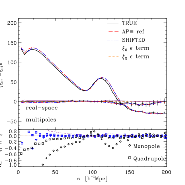
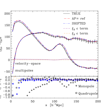
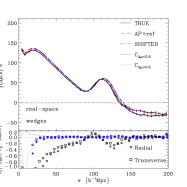
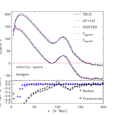
Figure 3: Mock mean clustering projections (based 160 LasDamas realizations) with and without the  AP effect. Left: real-space. Right: velocity-space. Top: multipoles (applying Equations 19, 20). Bottom: $\Delta\mu=1/2$ wedges (Equations 21-24). In the top panel of each plot are the 1D projections, and in the bottom panels the difference of each result with the DISTORTED signal (labeled as AP) normalized by the uncertainty of one realization. As indicated in legend, black solid lines/symbols are the true projection signals ($\,{\mathcal{T}}$), the long-dashed red lines are the AP signals ($\,{\mathcal{D}}$). We apply the AP shift to the true signals to obtain the triple-dot-dashed blue lines/symbols ($\,{\mathcal{S}}$). A perfect shift would yield a null result for the blue symbols in the bottom panels. The dot-dashed purple and dashed orange lines, as indicated in the legend, are the first order $\epsilon$ correction terms. The  AP distortion applied here is using $w^{\rm FID}=-1.1$ instead of the true value $-1$ when converting $z$ to comoving distances.

Our results are shown in Figure 3. The upper plots correspond to the results for the clustering multipoles and the bottom ones to the clustering wedges. The left plots show the measurements in real-space, and the right in velocity-space. Each plot consists of two panels. The top panels show $\xi\cdot s^{2}$ The $\xi^{\,{\mathcal{T}}}$ results are shown by solid black lines, the $\xi^{\,{\mathcal{D}}}$ results (called AP) are dashed red lines, and the $\xi^{\,{\mathcal{S}}}$ results are the dot-dashed lines. In the bottom panels, the $\xi^{\,{\mathcal{D}}}$ results form the reference to which we compare differences of $\xi^{\,{\mathcal{T}}}$ (black) and $\xi^{\,{\mathcal{S}}}$ (blue) in units of the uncertainty $\sigma_{\xi}$. In the multipoles the monopole results are in diamonds, and the quadrupole results are squares. In the wedges the radial wedge ($\Delta\mu>0.5$) results are in diamonds, and the transverse wedge ($\Delta\mu<0.5$) results are squares.

In the top left plot we see the  AP effect on the multipoles in real-space. We verify that the shift in the monopole from the $\xi^{\,{\mathcal{T}}}_{0}$ signal (solid) to the $\xi^{\,{\mathcal{D}}}_{0}$ (dashed) is described very well at zeroth order in $\epsilon$, meaning by $\xi_{0}^{\mathcal{D}}(s)\sim\xi_{0}^{\,{\mathcal{T}}}(\alpha s)$. Adding the warping $\epsilon$ terms adds little. In velocity-space, however, we do notice improvements when adding the first order correction at $s<50$ $h^{-1}$Mpc.

In real-space we do not expect signal in higher order multipoles. In Figure 3, though, there is a slight detection of $\xi_{2}$ and even $\xi_{\ell>2}$ measurements. These probably arise due to Poisson shot noise (either in the random points or data), or due to large angle effects. Nevertheless, we see that the  AP effect is understood for $\xi_{2}$ (Equation 20) in both real- and velocity-space. As expected in $\xi_{2}$, the $\alpha$ shift only is not sufficient, and adding the $\epsilon$ terms (blue) explain the  AP effect to high accuracy. We also test higher order corrections of $\xi_{4}$, d$\ln(\xi_{s})/$d$s$ in the quadrupole and find them negligible.

As for the $\xi_{4}$ statistics, we find that in velocity-space our corrections work well at $s>30$ $h^{-1}$Mpc. We argue that it does not work at smaller scales because we do not use the expected $\xi_{\ell>4}$ terms, which are required due to leakage of multipoles in the  AP effect.

We find similar trends for the clustering wedges statistics (bottom plots). In real-space (bottom left) we expect both $\xi^{\,{\mathcal{T}}}$ wedges to coincide. We notice minute differences at $130$ $h^{-1}$Mpc, (amplified in the plot by $s^{2}$ which make them visible). In velocity-space, as expected from the large quadrupole, there is a clear separation between the wedges, where the radial wedge is strongly suppressed and the transverse wedge elevated. The blue symbols indicate that the  AP is very well described by Equations (21)-(24). The first order correction terms ${\mathcal{C}}_{||,\perp}(\epsilon)$ (lines; see legend) are small ($\lesssim 1\%$ on most scales) with respect to the $\xi^{\,{\mathcal{T}}}$ wedge signals. This indicates that even with our definition of wide “radial” and “transverse” wedges ($\Delta\mu=0.5$), the radial wedge is mostly sensitive to $H$, while the transverse wedge to $\,D_{\rm A}$. That said, in Appendix B we show that although setting ${\mathcal{C}}_{||,\perp}(\epsilon)=0$ yields fairly accurate $H,\ \,D_{\rm A}$ results, including ${\mathcal{C}}_{||,\perp}(\epsilon)$ can improve the results.

To summarize this test, we have proven here that  AP effects on the clustering multipoles and wedges are very well understood. We show that the dilation and warping terms shown by  Padmanabhan & White (2008) explain this effect very well in the monopole and quadrupole of the two-point correlation function. In addition we show an alternative approach to measuring the  AP effect by analyzing clustering wedges. We show here that even a wide “radial” wedge is, as expected, mostly sensitive to $H$ and a wide “transverse” wedge to $\,D_{\rm A}$. In Appendix C we perform similar tests on analytic formulae and obtain similar conclusions. In the next section we investigate the power of this method to obtain constraints on $H$ and $\,D_{\rm A}$ from measurements of the multipoles and wedges.

4.2 Reproducing the true $H$ and $\,D_{\rm A}$

Here we perform the  AP test on the LRG SDSS-II mock catalogues described in §2.2 to measure $H$ and $\,D_{\rm A}$. When quoting uncertainties in these parameters, we show what might be expected for a survey with the same number density as SDSS-II ($n\sim 10^{-4}\,h^{3}\rm{Mpc}^{-3}$) but a volume twelve times larger, corresponding to the total Hubble volume (i.e, a sphere of radius $c/H_{0}$).

To simulate the observer’s point of view, we assume the $\xi^{\,{\mathcal{D}}}$ measurements to be the “data” points. We then find the best fitting models based on physical templates. Our first step is to perform an ideal test, where the template is the $\xi^{\,{\mathcal{T}}}$ mock mean signal. In other words, we are not concerning ourselves, at this point, with uncertainties beyond the  AP effect. For example, this means we assume that we fully understand the amplitude “bias”, and dynamical $z$-distortions. We consider this merely as a “proof of concept” of the analysis, and in §4.3 take a more realistic approach by adding more unknowns.

In §2.1 we describe the construction of the covariance matrix, in which we take into account covariances between the statistics. When manipulating the template, the covariance matrix is not varied, but rather fixed to the true cosmology. Samushia et al. (2011) discuss the sensitivity of $C_{ij}$ to amplitude parameters and its insensitivity to shape parameters.

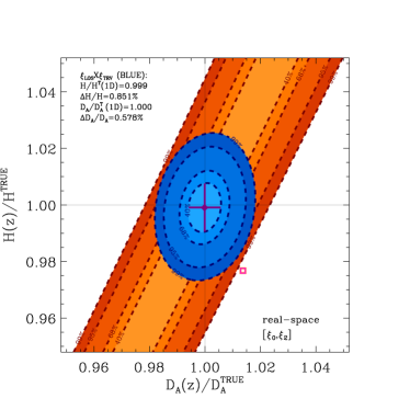
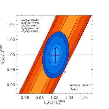
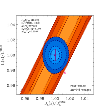
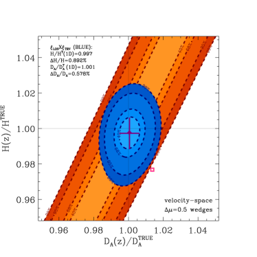
Figure 4: $H-\,D_{\rm A}$ joint constraints from  AP shift tests when analyzing mock mean clustering 1D statistics. Left panels: real-space. Right: velocity-space. The blue ellipses correspond to analysis of [$\xi_{0},\xi_{2}]$ (top panels) and $\Delta\mu=1/2$ wedges (bottom). The orange bands are the results when analyzing only the $\xi_{0}$. The parameter space tested is $\Phi=$[$\,D_{\rm A}$,$H$], where amplitude remains fixed (“ AP only”). The true cosmology of the simulations corresponds to [1,1], and the distortion cosmology tested when converting redshifts to comoving distances (pink box) corresponds to using $w^{\mathcal{D}}=-1.1$ instead of the true $-1$ value, and is the same for all tests. The even contour likelihood mock mean values are for $40,\ 68.3,\ 95.4,\ 99\%$ CL. The most likely 2D values are purple diamonds, and the 1D marginalized $1\sigma$ results are the purple crosses. On the top of each plot we inscribe for each parameter $\Phi$ the deviation from the true value in the 1D marginalized results, as well as $\Delta\Phi/\Phi$. The constraints correspond roughly to a fictitious survey with a Hubble volume ($R\sim c/H_{0}$) and a galaxy density of $n\sim 10^{-4}(h/{\rm Mpc})^{3}$.

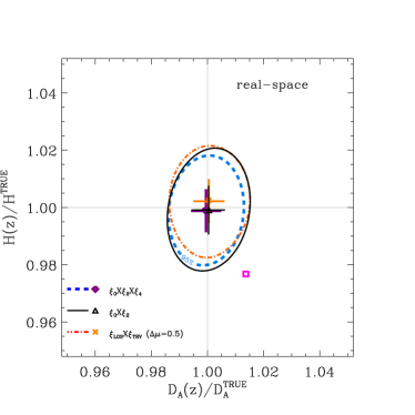
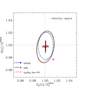
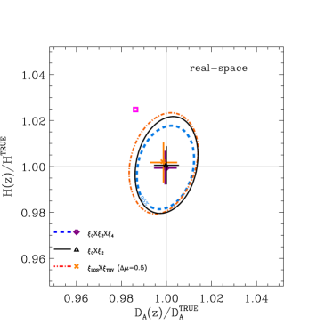
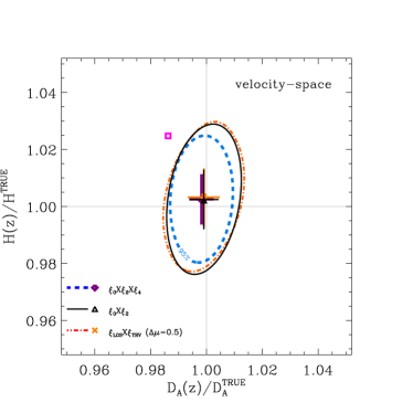
Figure 5: Joint $2\sigma$ constraints on the $H-\,D_{\rm A}$ plane from  AP shift tests when analyzing mock mean clustering 1D statistics. Left panels: real-space. Right: velocity-space. The  AP distortion tested is when using $w^{\mathcal{D}}$ different from the true value $w^{\mathcal{T}}=-1$ when converting redshifts to comoving distances. Top panels show results for $w^{\mathcal{D}}=-1.1$, and bottom panels for $w^{\mathcal{D}}=-0.9$ (notice difference in input fiducial cosmology indicated by the magenta squares). The Parameter space analised is [$\,D_{\rm A}$,$H$], where the amplitude remains fixed (“ AP only”). The dashed blue lines correspond to the constraints for the multipole combination [$\xi_{0},\xi_{2},\xi_{4}$], solid black lines to [$\xi_{0},\xi_{2}$], and dot-dashed orange lines to $\Delta\mu=1/2$ wedges. Crosses indicate marginalized $1\sigma$ results according to color, and symbols most likely 2D value. The $w^{\mathcal{D}}=-1.1$ clustering wedges and [$\xi_{0},\xi_{2}$] results are the same as the blue ellipses in Figure 4. Adding the hexadcapole information clearly improves constraints. These constraints correspond roughly to a fictitious survey with a Hubble volume ($R\sim c/H_{0}$) and a galaxy density of $n\sim 10^{-4}(h/{\rm Mpc})^{3}$.

Our results are presented in Figures 4-5. Figure 4 shows the two-dimensional marginalized constraints on the $\,D_{\rm A}-H$ plane. The contours shown correspond to 40, 68, 95, and 99% confidence levels. The best fit values of each parameter and their respective $1\sigma$ (68%) CL regions after marginalizing over the other are indicated by the purple crosses. We find that the best fit model recovers, to high accuracy, the true values of these parameters. The pink box corresponds to the fiducial cosmology. In the legend we display the calculated deviations from the true values in the 2D analysis (purple diamond). We also note the marginalized uncertainty for (i.e, the analog of the diagonal elements in Fisher-Matrix analysis). For the wedges we make use of first order correction terms ${\mathcal{C}}_{\perp,||}(\epsilon)$, and in Appendix B discuss their importance. For comparison, the wide orange contours display the constraining power of the monopole on its own. The result is the well known $\,D_{\rm A}^{2}/H$ degeneracy.

The fitting range chosen here is $40<s<150$ $h^{-1}$Mpc in bins of $\Delta s=5$ $h^{-1}$Mpc. As discussed in Sánchez et al. (2008) and Shoji et al. (2009), we find that the extra information included when analyzing larger ranges yields tighter constraints.

We notice that in all cases the true parameters are recovered to high accuracy, and the input incorrect cosmology is ruled out by over $3\sigma$ solely by the  AP effect on clustering. That said, this level of precision is not expected when using this technique in near future galaxy samples, because marginalization over a larger parameter space would be required. We discuss this more detail in §4.3.

We do notice, though, differences in the results obtained by means of the two projection techniques. We emphasize that these are fair tests, as every step along the analysis is equivalent as much as possible. When analyzing real-space information (left plots), we see that $\,D_{\rm A}$ is measured to similar accuracy with both techniques, with the clustering wedges yielding slightly smaller uncertainties. Interestingly, the differences in the recovery of $H$ between the two methods are larger where the clustering wedges yield a more accurate result, as well as smaller uncertainties. Throughout this study we compare these statistics, and find that the clustering wedges defined by $\Delta\mu=1/2$ perform better than $\xi_{0},\xi_{2}$, for the most part, and motivate adding $\xi_{4}$ to improving constraints when using multipoles.

In the plots on the right we compare the performance of these statistics in velocity-space. Most notable is the fact that the uncertainties in $H$ increase substantially for both projection pairs compared to real-space results. Although the wedges yield tighter uncertainties in $H$, the multipoles generate slightly more accurate results. As for $\,D_{\rm A}$ they both yield similar uncertainties, but clustering wedges yield more accurate results, and do not change much from real-space.

When fitting for the $\Delta\mu=1/2$ clustering wedges, we take into account the intermixing terms ${\mathcal{C}}_{||,\perp}$ (Equations 23 and 24). In Appendix B we explore their effectiveness and test results obtained by other wedge widths. We find that setting ${\mathcal{C}}_{||,\perp}=0$ (meaning radial wedge depends solely on $H$ and transverse wedges solely on $\,D_{\rm A}$), yields results that are less accurate and uncertainties that are underestimated. We also find that the ${\mathcal{C}}_{||,\perp}$ terms are less important as one decreases $\Delta\mu$.

In the top panels of Figure 5 we compare the results shown in Figure 4 with ones obtained when adding $\xi_{4}$ to the multipole pair. The bottom plots corresponds to the same test but using a different choice for the fiducial cosmology ($w=-0.9$; notice the different location of the magenta box). The left plots are in real-space and the right in velocity-space.

In all cases the true cosmology is recovered to high accuracy. As expected, the $[\xi_{0},\xi_{2},\xi_{4}]$ combination (dash blue lines) yields tighter constraints than when limiting the analysis to $[\xi_{0},\xi_{2}]$ (solid black lines) or the $\Delta\mu=0.5$ wedges (dot-dashed orange lines). Crosses indicate marginalized $1\sigma$ results according to color, and symbols most likely 2D value. The real-space $w=-0.9$ result (bottom left plot) shows that the wedges do not generically yield tighter constraints than the monopole-quadrupole pair. In velocity-space, we notice that adding the $\xi_{4}$ information in the multipoles yields a smaller correlation coefficient between $H$ and $\,D_{\rm A}$.

Another oddity is the fact that in real-space $\xi_{4}$ is present at all, and can assist in improving constraints. We argue that it is probably an artifact of angular effects at large scales (see §4.1). We verify this by limiting our analysis to the range $s=[20,60]$ $h^{-1}$Mpc, finding less of an improvement when using $\xi_{4}$, as its angular effect is negligible at these scales. These suggest that including $\xi_{4}$ is useful in breaking the $H-\,D_{\rm A}$ degeneracy in velocity-space.

To summarize the results of this section, we find that in the ideal case analysed here the true parameters are recovered to high accuracy with both statistics. The input incorrect cosmology is ruled out by over $3\sigma$ solely by the  AP effect on clustering. We demonstrate here, for the first time, the power of the clustering wedges technique. We find that using Equations (21) and (22) to describe the  AP distortions in the clustering wedges it is possible to recover the true parameters as well as one can with the multipole expansion. This means that even a wide “radial” wedge is most sensitive to $H$ while a “transverse” wedges is most sensitive to $\,D_{\rm A}$. We also demonstrate that adding $\xi_{4}$ to the multipoles substantially improves constraints.

4.3 Amplitude effects on uncertainties

In the previous sections we simulate “ideal” observational tests, in which the correlation function template from which the models are constructed, is fully understood except for the  AP effect. Here we address the fact that the observer does not have the luxury of knowing the correct signal a priori.

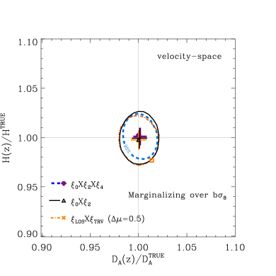
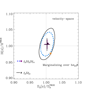
Figure 6: Joint $2\sigma$ constraints on $H-\,D_{\rm A}$ from  AP shift tests when analyzing mock mean velocity-space clustering 1D statistics. The parameter space in the upper panel is $\Phi=[\,D_{\rm A},H,b\sigma_{8}]$. and $\Phi=[\,D_{\rm A},H,b\sigma_{8},\beta]$ in the bottom. The analysis of the results shown here is similar to that performed when producing the results shown in Figure 5 only marginalizing over amplitude parameters. $H-\,D_{\rm A}$ joint constraints for the multipole combination [$\xi_{0},\xi_{2},\xi_{4}$] are shown in dashed blue lines, [$\xi_{0},\xi_{2}$] are in solid black lines, and $\Delta\mu=1/2$ wedges are dot-dashed orange lines. Crosses indicate marginalized $1\sigma$ results according to color, and symbols most likely 2D value. The  AP distortion applied here is using $w^{\rm FID}=-1.1$ (orange box) instead of the true value $-1$ when converting $z$ to comoving distances. These constraints roughly correspond to a fictitious survey with a Hubble volume ($R\sim c/H_{0}$) and a galaxy density of $n\sim 10^{-4}(h/{\rm Mpc})^{3}$.

To mention a few main concerns, one must understand the $\xi$ amplitude, shape, and various effects on the angular  baryonic acoustic feature. The amplitude may be scale dependent for various reasons: non-linear tracer-matter bias, scale dependent dynamic distortion effects, observer angular effects, magnification bias (Hui et al. 2007) and effects of non-gaussianities in initial conditions (Dalal et al. 2008).

Here we take into account the effect of uncertainties in the amplitudes of the various statistics and leave shape effects for a future study. For this, we add amplitude parameters to the $H-\,D_{\rm A}$ parameter space. We assume that the amplitudes of the multipoles and clustering wedges are given by $A_{{\rm stat}}=B_{{\rm stat}}\,b^{2}\,\sigma_{8}^{2}$, where $b$ is the (scale-independent) bias parameter of the tracer with respect to the matter, $\sigma_{8}$ is the rms linear perturbation theory variance in spheres of radius $8$ $h^{-1}$Mpc, and $B_{\rm stat}$ is the Kaiser squashing amplitude on large scales, which in real-space is unity. The subscript “stat” signifies the fact that we test for various statistics such as the wedges and multipoles.

For the multipoles in velocity-space $B_{\rm stat}$ is given by the usual Kaiser (1987) prefixes

$$B_{0} = 1+2/3\beta+1/5\beta^{2},$$ (25)

$$B_{2} = 4/3\beta+4/7\beta^{2},$$ (26)

$$B_{4} = 8/35\beta^{4},$$ (27)

of the squashing parameter $\beta(z)\equiv f/b\sim\Omega_{\rm M}(z)^{0.55}/b$, where $f\equiv d\ln(D_{1})/d\ln(a)$, with $D_{1}$ the standard linear growth factor and and $a$ the scale factor. Technically, as the templates used here correspond to the $\,{\mathcal{T}}$ signal, when testing for the amplitude the models are based on the ratio of $A_{\rm stat}$ to its real value.

When testing for $b\sigma_{8}$ we perform the analysis on wedges and multipoles. When testing for $\beta$, however, this is a non-trivial task for the wedges. This is due to the volume averaged monopole term which makes it non-trivial to account for $A_{\rm stat}$ in configuration space (see the terms involving $\overline{\xi}$ in equations 6-8 of Hamilton 1992). In a $k-$space analysis this issue would be trivial, as it should be when building a generic model, which we do not do here. For this reason, results shown marginalizing over $\beta$ are limited to multipoles. The fiducial $\beta$ tested is calculated through the input $f(z)$ and the linear $b\sim 1.96$ which is inferred from matching linear theory to the standard projected correlation function $w_{p}(s_{\perp})$ of the mocks.

In Figure 6 we show joint constraints on $H$ and $\,D_{\rm A}$ using the various statistics when marginalizing over $b\sigma_{8}$ (top) and [$b\sigma_{8},\beta$] (bottom). For the former case we assume perfect knowledge of the dynamic distortions, whereas for the latter we add the uncertainty of the Kaiser effect (disregarding velocity dispersion). The obtained constraints can be compared with those of Figure 5, and show a clear degradation of the uncertainties on $H$ nearly by a factor of two and a slight degradation of the uncertainties on $\,D_{\rm A}$ with respect to the results obtained without uncertainties in the amplitudes. In §4.4 we study the effect of varying the range of scales included in the analysis. These plots show fair comparisons between [$\xi_{0},\xi_{2}$], [$\xi_{0},\xi_{2},\xi_{4}$] and $\Delta\mu=0.5$ clustering wedges.

We see that the true cosmology is recovered to high accuracy, but our choice of incorrect cosmology $w=-1.1$ is ruled out by [$\xi_{0},\xi_{2}$] at only $2\sigma$ (top) and $\sim 1.5\sigma$ (bottom), due to the marginalization over the amplitude parameters. The importance of the first finding is that multipole  AP Equations (19) and (20), hold to a very good degree. We obtain similar conclusions for Equations (21), (22) and (23) regarding the clustering wedges. As in the test performed in §4.2, we find an increase in the uncertainties of $H$ at the $10\%$ level when going from real- to velocity-space.

To conclude these tests we find that increasing the allowed range of the amplitude parameters degrades the constraints, but retains accuracy in recovering the true values of $H$ and $\,D_{\rm A}$. When comparing between the different statistics our conclusions of this test are similar to those obtained in §4.2. We demonstrate that $\xi_{4}$ improves constraints substantially compared to those obtained when limited to monopole-quadrupole.

4.4 Wedges or multipoles?

In §4.2 and §4.3 we analyse a particular case where the constraining power on $H$ of the $\Delta\mu=0.5$ clustering wedges outperforms the monopole-quadrupole pair, and see substantial improvement when including the hexadecapole (see Figure 5). However, in these analyses we limit the range of scales to $40<s<150$ $h^{-1}$Mpc. Here we generalize these tests by varying the minimum scale included in the analysis $s_{\rm min}$ while keeping the maximum scale fixed to $s_{{\rm max}}=150$ $h^{-1}$Mpc, and find interesting trends for the constraining power of the various statistics. All results given here are in velocity-space.

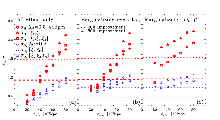
Figure 7: Relative uncertainties $\sigma_{H}/H$ and $\sigma_{D_{\rm A}/\,D_{\rm A}}$ as a function of the range analysed [$s_{\rm min}$, $150$ $h^{-1}$Mpc] (given in $[\%]$). The different symbols, indicated in the legend, represent the various 1D statistics used. Thick red symbols are for $\sigma_{H}$, and thin blue for $\sigma_{\,D_{\rm A}}$. (a): “ AP only”- $[H,\,D_{\rm A}]$ with fixed amplitude. (b): $[H,\,D_{\rm A}]$ when marginalizing over $b\sigma_{8}$ without prior. (c): $[H,\,D_{\rm A}]$ when marginalizing over $b\sigma_{8},\beta$ without prior. Slopes indicate the improved constraints obtained by using information from the broad band of $\xi$. The dotted lines indicate an improvement of $0.8$ from $\sigma_{\Phi}/\Phi(s_{\rm max}=80\ h^{-1}{\rm Mpc})$ (when fitting for [$\xi_{0},\xi_{2},\xi_{4}$]; $\Phi=[H,\,D_{\rm A}]$), and the dashed lines an improvement of $0.5$. The  AP distortion applied here is using $w^{\rm FID}=-1.1$ instead of the true value $-1$ when converting $z$ to comoving distances.

Our findings are summarized in Figure 7, in which we show the uncertainties on $H$ and $\,D_{\rm A}$ as a function of $s_{\rm min}$.

Results for an “ AP effect only” are displayed in Figure 7a, which generalize the top right plot in Figure 5. “ AP only” refers to tests in which we fix amplitude parameters to their true values and test only for $H$ and $\,D_{\rm A}$. When marginalizing over $b\sigma_{8}$ we obtain results displayed in Figure 7b, which generalizes the top plot of Figure 6. Figure 7c shows the results obtained when marginalizing over both $b\sigma_{8}$ and $\beta$, and is a generalization of the bottom plot of Figure 6. No priors are assumed for $b\sigma_{8}$ or $\beta$.

In all cases we find that adding information from $\xi_{4}$ to the multipole analysis improves the obtained constraints on $H$ and $D_{\rm A}$ by a substantial amount.

The improvement in the constraints as smaller scales are included in the analysis emphasizes the fact that although the  baryonic acoustic feature is essential to perform the  AP test, one can extract more information by analyzing the full broad shape of $\xi$ (Sánchez et al., 2008; Shoji et al., 2009).

In all parameter spaces tested, the slope of $\sigma_{H}(s_{\rm min})$ (thick red) is steeper than that of $\sigma_{\,D_{\rm A}}$ (thin blue), indicating that the broad shape of these statistics is more sensitive to $H$. The fact that the “ AP only” test (Figure 7a) has steeper slopes than the others is expected. In this case each data point posses a high constraining power.  Padmanabhan & White (2008) explain that marginalizing over the amplitude is somewhat degenerate with the  AP effect and hence leads to a reduction of the slope when adding $b\sigma_{8}$ (Figure 7b) and even more when adding $\beta$ (Figure 7c). Nevertheless, even when marginalizing over $b\sigma_{8}$ we notice an improvement of factor two in the uncertainty on $H$ and a factor of $\sim 1.25$ in $\sigma_{\,D_{\rm A}}$ when using the full information up to $40$ $h^{-1}$Mpc, with respect to setting $s_{\rm min}=80$ $h^{-1}$Mpc (i.e, focusing on the scales around the  baryonic acoustic feature).

The answer to the question of which statistics should be preferred is not simple as it appears to depend on the range of scales used. For high values of $s_{\rm min}$ the results obtained by means of the clustering wedges (diamonds) outperform those obtained with the $[\xi_{0},\xi_{2}]$ combination (triangles). However, we notice the different slopes of $\sigma_{\,D_{\rm A}}(s_{\rm min})$ and $\sigma_{H}(s_{\rm min})$ such that the multipole pair should be preferred when a large range of scales is considered (i.e. low $s_{\rm min}$).

A puzzling result is the fact that $\sigma_{\,D_{\rm A}}(s_{\rm min})$ and $\sigma_{H}(s_{\rm min})$ have a steeper slope for the case of the $[\xi_{0},\xi_{2},\xi_{4}]$ combination than for the clustering wedges. The $\sigma_{H}(s_{\rm min})$ results indicate that the $\Delta\mu=0.5$ wedges are preferred at $s_{\rm min}>50$ $h^{-1}$Mpc (although $[\xi_{0},\xi_{2},\xi_{4}]$ is preferred to determine $\,D_{\rm A}$). This might be explained by angular effects causing higher multipoles, which we have not corrected for properly with the multipoles, but happen not to affect the wedges, which are combinations of all multipoles.

For this analysis we have chosen $w^{\rm fid}=-1.1$ of our fiducial cosmology (instead of $w^{\rm true}=-1$). When testing for $w^{\rm fid}=-0.9$ we find similar trends but with varying crossover points. For example, in the “ AP only” case, the clustering wedges are preferred over the [$\xi_{0},\xi_{2},\xi_{4}$] combination in determining $H$ at $s_{\rm min}>55$ $h^{-1}$Mpc instead of $>45$ $h^{-1}$Mpc.

5 Predicted Constraints on $H$ and $\,D_{\rm A}$ from BOSS

Here we apply both the multipole and wedge techniques to the 32 realizations of the Horizon Run mock galaxy catalogues described in §2.2, which serve as simulated realizations of the final BOSS volume. We investigate the accuracy with which $H$ and $\,D_{\rm A}$ can be obtained for a survey covering $10,000$ square degrees in the redshift range $0.16<z<0.6$ with density $n\sim 3\cdot 10^{-4}h^{3}$Mpc^-3. For full details of the mocks please refer to §2.2. Analyzing $32$ realizations, we obtain results for the full sample, and of for two subsamples split at $z=0.45$. This redshift split is motivated by the so-called targeted LOWZ and CMASS BOSS galaxies (see Eisenstein et al. 2011 and Padmanabhan et al. (in prep.)).

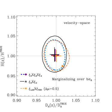
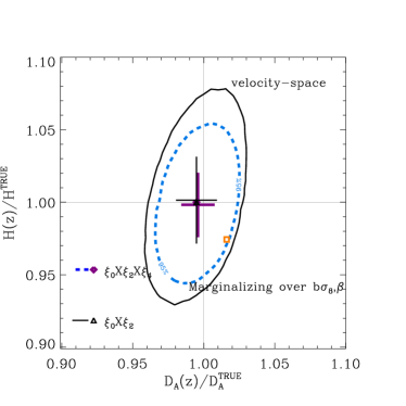
Figure 8: BOSS mock galaxy mean ($0.16<z<0.6$) $H-\,D_{\rm A}$ joint $2\sigma$ constraints from  AP shift tests, when analyzing velocity-space clustering 1D statistics. The parameter space in the left panel is [$\,D_{\rm A}$,$H$,$b\sigma_{8}$]. and [$\,D_{\rm A}$,$H$,$b\sigma_{8}$,$\beta$] in the right. $H-\,D_{\rm A}$ joint constraints for the multipole combination [$\xi_{0},\xi_{2},\xi_{4}$] are shown in dashed blue lines, [$\xi_{0},\xi_{2}$] are in solid black lines, and $\Delta\mu=1/2$ wedges are dot-dashed orange lines. Crosses indicate marginalized $1\sigma$ results according to color, and symbols most likely 2D value. The  AP distortion applied here is using $w^{\rm FID}=-1.1$ (orange box) instead of the true value $-1$, when converting $z$ to comoving distances. These constraints correspond to an analysis of the broadband $s=[40,150]$ $h^{-1}$Mpc, without priors, and assumes all shape effects are fully understood. In both [$\xi_{0},\xi_{2},\xi_{4}$] cases the true cosmology is recovered with excellent accuracy, and the incorrect input $H,\,D_{\rm A}$ is rejected by $\sim 2\sigma$. We clearly see a degradation in constraining $H$ when including marginalization of $\beta$.

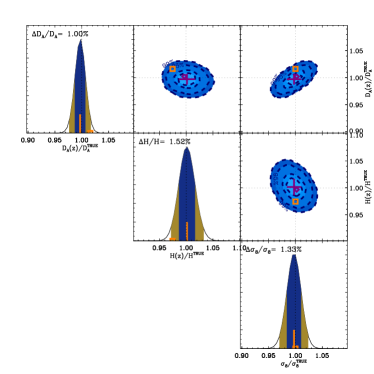
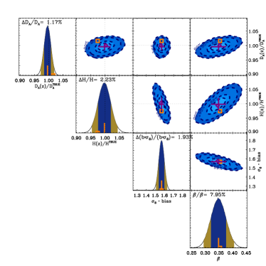
Figure 9: BOSS mock galaxy mean ($0.16<z<0.6$) joint and marginalized constraints from  AP shift tests, when analyzing velocity-space clustering [$\xi_{0},\xi_{2},\xi_{4}$]. (These results are the same as those displayed in Figure 8, meaning analyzing region $s=[40,150]$ $h^{-1}$Mpc). The parameter space in the left panel is [$\,D_{\rm A}$,$H$,$b\sigma_{8}$]. and [$\,D_{\rm A}$,$H$,$b\sigma_{8}$,$\beta$] in the right. The joint constraints are for CL: [$40,68,95,99$]$\%$. On the top of each 1D likelihood plot we inscribe for each parameter $\Phi$ the marginalized $1\sigma$ result, also summarized in Table 1. The orange boxes demonstrate the fiducial parameters input into the analysis (in the case of $H$ and $\,D_{\rm A}$ this is the  AP effect using $w^{\rm FID}=-1.1$ instead of the true $-1$ value when converting redshifts to comoving distances). In all cases the true cosmology is recovered with excellent accuracy, and the incorrect input $H,\,D_{\rm A}$ is rejected by $\sim 2\sigma$. We clearly see a $\sim 30\%$ degradation in constraining $H$ when including marginalization of $\beta$, and a $\sim 15\%$ degradation in $\,D_{\rm A}$.

As in previous sections, when building our templates, we gradually increase our parameter space, starting from solely the  AP effect and adding amplitude parameters. For each case we analyse both real- and velocity-space and obtain the corresponding results as expected from one BOSS volume.

On a technical note, the mock “data” and templates are based on the mock mean of $32$ Horizon Run mocks. To obtain a stable, invertible $C_{ij}$ we use the $160$ LasDamas mocks, normalized by the variance of the $32$ Horizon Run mocks.

Our $0.16<z<0.6$ results are shown in Figures 8 and 9 for a particular range $40<s<150$ $h^{-1}$Mpc. The left plots in each figure are results for the parameter space [$H,\,D_{\rm A},b\sigma_{8}$] and the right plots for [$H,\,D_{\rm A},b\sigma_{8},\beta$]. Figure 8 compares the statistic combinations in the $H-\,D_{\rm A}$ plane. In Figure 9 we display one and two-dimensional likelihood functions for the above three and four parameter spaces when using the [$\xi_{0},\xi_{2},\xi_{4}$] combination. Marginalized $1\sigma$ uncertainty values are indicated on the 1D likelihood panels. In Table 1 we summarize the $1\sigma$ uncertainty values obtained for the various statistic combinations, parameter spaces, choices of $s_{\rm min}$, and sample analysed.

In all cases investigated we find that the true cosmology ($H,\,D_{\rm A}$) is recovered to high accuracy (much better than $1\%$). We report that the velocity-space results yield a noticeable increase in uncertainty of $H$ compared to real-space results. Below we will limit our explanations to velocity-space results.

When allowing the amplitude parameters to vary, we find that uncertainties in the $H-\,D_{\rm A}$ plane are degraded, as expected. When adding $\beta$ in velocity-space, we notice an increase in the uncertainty of $H$ by a fraction range of $1.1$ to $1.6$, depending on the scales included in the analysis. For $\,D_{\rm A}$ the fraction changes by $1.01$ to $1.10$.

Table 1: BOSS predictions based on velocity-space Horizon Run mock galaxies^a

Parameter Space	1D Projection	Volumeb	analysis range  $h^{-1}$Mpc	$\sigma_{H}/H$ $\%$ c	$\sigma_{\,D_{\rm A}}/\,D_{\rm A}$ $\%$ c
AP onlyd	$[\xi_{0},\xi_{2}]$	$0.16<z<0.6$	$[40,150]$	$1.71$	$0.90$
AP only	$[\xi_{0},\xi_{2},\xi_{4}]^{e}$	$0.16<z<0.6$	$[40,150]$	$1.41$	$0.72$
AP only	$\Delta\mu=1/2$ wedges	$0.16<z<0.6$	$[40,150]$	1.33	$0.99$
AP, $b\sigma_{8}$	$[\xi_{0},\xi_{2}]$	$0.16<z<0.6$	$[40,150]$	$1.82$	$1.24$
AP, $b\sigma_{8}$	$[\xi_{0},\xi_{2},\xi_{4}]$	$0.16<z<0.6$	$[40,150]$	$1.52$	$1.00$
AP, $b\sigma_{8}$	$\Delta\mu=1/2$ wedges	$0.16<z<0.6$	$[40,150]$	1.52	$1.25$
AP, $b\sigma_{8}$	$[\xi_{0},\xi_{2}]$	$0.16<z<0.6$	$[60,150]$	$3.13$	$1.52$
AP, $b\sigma_{8}$	$[\xi_{0},\xi_{2},\xi_{4}]$	$0.16<z<0.6$	$[60,150]$	$2.28$	$1.32$
AP, $b\sigma_{8}$	$\Delta\mu=1/2$ wedges	$0.16<z<0.6$	$[60,150]$	2.44	$1.48$
AP, $b\sigma_{8}$, $\beta$	$[\xi_{0},\xi_{2}]$	$0.16<z<0.6$	$[40,150]$	$2.99$	$1.44$
AP, $b\sigma_{8}$, $\beta$	$[\xi_{0},\xi_{2},\xi_{4}]$	$0.16<z<0.6$	$[40,150]$	$2.24$	$1.17$
AP, $b\sigma_{8}$, $\beta$	$[\xi_{0},\xi_{2}]$	$0.16<z<0.6$	$[60,150]$	$3.45$	$1.57$
AP, $b\sigma_{8}$, $\beta$	$[\xi_{0},\xi_{2},\xi_{4}]$	$0.16<z<0.6$	$[60,150]$	$2.53$	$1.35$
AP, $b\sigma_{8}$	$[\xi_{0},\xi_{2}]$	$0.16<z<0.45$	$[40,150]$	$2.42$	$1.85$
AP, $b\sigma_{8}$	$[\xi_{0},\xi_{2}]$	$0.45<z<0.60$	$[40,150]$	$2.43$	$1.67$
AP, $b\sigma_{8}$	$[\xi_{0},\xi_{2},\xi_{4}]$	$0.16<z<0.45$	$[40,150]$	2.13	1.46
AP, $b\sigma_{8}$	$[\xi_{0},\xi_{2},\xi_{4}]$	$0.45<z<0.6$	$[40,150]$	1.85	1.41
AP, $b\sigma_{8}$	$\Delta\mu=1/2$ wedges	$0.16<z<0.45$	$[40,150]$	2.22	$1.81$
AP, $b\sigma_{8}$	$\Delta\mu=1/2$ wedges	$0.45<z<0.6$	$[40,150]$	2.19	$1.60$
AP, $b\sigma_{8}$, $\beta$	$[\xi_{0},\xi_{2}]$	$0.16<z<0.45$	$[40,150]$	$4.05$	$2.95$
AP, $b\sigma_{8}$, $\beta$	$[\xi_{0},\xi_{2}]$	$0.45<z<0.60$	$[40,150]$	$3.84$	$2.00$
AP, $b\sigma_{8}$, $\beta$	$[\xi_{0},\xi_{2},\xi_{4}]$	$0.16<z<0.45$	$[40,150]$	3.23	1.61
AP, $b\sigma_{8}$, $\beta$	$[\xi_{0},\xi_{2},\xi_{4}]$	$0.45<z<0.6$	$[40,150]$	2.79	1.70

^a We use the $C_{ij}$ based on 160 LasDamas (SDSS-II LRG) mocks normalized by the $C_{ii}$ of 32 Horizon Run (BOSS) mocks.

^b All BOSS mocks are volume limited and cover 1/4 of the sky with $n\sim 3\cdot 10^{-4}h^{3}$Mpc^-3. For $0.16<z<0.6$: $V=4$ $h^{-3}{\rm Gpc}^{3}$, $0.16<z<0.45$: 1.8  $h^{-3}{\rm Gpc}^{3}$, $0.45<z<0.6$: 2.2  $h^{-3}{\rm Gpc}^{3}$.

^c $1\sigma$ meaning $68.4\%$ CL when all other parameters marginalized over.

^d “ AP only” means amplitude is fixed and we test for $H$, $\,D_{\rm A}$.

^e Analyses of $\xi_{4}$ assume it can be measured and modeled for. In BOSS, we do, however, expect low S/N at  baryonic acoustic feature scales.

As in the previous sections, we find in all cases that adding the $\xi_{4}$ information imporves the constraints obtained by means of the multipoles. We see an improvement of a factor $1.2$ to $1.35$ in $H$ and between $1.15$ to $1.25$ in $\,D_{\rm A}$. This is comparable to results found in Taruya et al. (2011), who perform a Fisher Matrix analysis.

As for the clustering wedges, we find that they outperform the monopole-quadrupole pair in $H$ while giving similar constraints on $\,D_{\rm A}$. Interestingly, in this case the $\Delta\mu=0.5$ clustering wedges measure $H$ with a similar accuracy to that of $[\xi_{0},\xi_{2},\xi_{4}]$.

As to values expected from BOSS, we find that, assuming that $\beta$ is fixed and the broad shape understood down to $40$ $h^{-1}$Mpc, our best $0.16<z<0.6$ constraints obtained are: $\Delta H/H\sim 1.52\%$ (similar for wedges and [$\xi_{0},\xi_{2},\xi_{4}$]) and $\Delta\,D_{\rm A}/\,D_{\rm A}\sim 1\%$ ([$\xi_{0},\xi_{2},\xi_{4}$]).

When splitting to the two subsamples, using [$\xi_{0},\xi_{2},\xi_{4}$] at $40<s<150$ $h^{-1}$Mpc, NEAR yields [$\Delta H/H,\Delta\,D_{\rm A}/\,D_{\rm A}$]$\sim[2.13,1.46]\%$ and FAR [$1.85,1.41\%$].

Schlegel et al. (2009) use Fisher-Matrix analysis to obtain much more optimistic estimates, than those shown here, even though they focus on the baryonic acoustic wiggles in $P(k)$, and not the broad shape and do not use the $\xi_{4}$. This is probably due to the fact that they assume the “reconstruction” of the feature which, if applicable without introducing bias, should improve the obtained constraints (Eisenstein et al. 2007). We have not applied the technique on the mocks.

6 Discussion

The purpose of this study is to investigate possible ways to break the $H-\,D_{\rm A}$ degeneracy by including information in the anisotropy in the $\xi(\mu,s)$ plane produced by geometrical redshift distortions.

6.1 Relating our analysis to previous studies

This concept has been studied in the full 2D $P(\mu,k)$ plane by Hu & Haiman (2003), Wagner et al. (2008), and Shoji et al. (2009), who investigated the power of using the  baryonic acoustic feature to determine the equation of state of dark energy. In practical terms, however, there are a few difficulties in applying this approach on real data, namely the low S/N of the measurements in the full $\mu-k$ plane, the practical problems related to estimating accurate covariance matrices for them, and the difficulties in constructing realistic models that take non-linearities into account.

Following  Padmanabhan & White (2008) and Taruya et al. (2010), we break the $H-\,D_{\rm A}$ degeneracy by using projections of the $\mu-s$ plane, which have the advantage of a higher S/N, while preserving much of the essential information. As near future surveys will provide fairly noisy $P(\mu,k)$ planes, we find the projection approach more useful in the short term.

These last two studies focused on the monopole-quadrupole (or “multipole”) pair in $k-$space. We demonstrate similar results for the first time in configuration space, and introduce an alternative method in the form of clustering wedges $\xi(\Delta\mu,s)$, and compare their constraining power to that of the multipoles.

The projection approach also simplifies covariance issues, as one resorts to a much smaller covariance matrix, which is more likely to be invertible and stable, when using a reasonable number of mock realizations. An alternative method suggested by Taruya et al. (2010) is to ignore non-Gaussianties by using a linear Cov${}_{\ell,\ell^{\prime}}(k)$ based on an analytic model. While this might be a fine approach for simple estimates, when analyzing real data one should take into account observational effects, most straightforwardly achieved by mock realizations with a similar window function, such as the mock catalogues produced by the LasDamas group (McBride et al.; in prep), and used here.

In this study we analyse geometric effects (or  AP effects after Alcock & Paczynski 1979) in clustering. We study the effect of using an incorrect value for the dark-energy equation of state $w$, when converting redshifts to comoving distances, causing slight shifts in the inferred positions of the galaxies in respect to the real positions. Instead of the true $w=-1$ value we use $-0.9$ and $-1.1$, which is within the allowed region for this parameter according to current observations (Komatsu et al. 2009, Sánchez et al. 2009, Percival et al. 2010, Reid et al. 2010). It is interesting to note that the $-0.9$ shift (which causes larger dilations and warps) yields slightly, but noticeable, larger uncertainties in both real- and velocity-space (to see this compare the corresponding results in Figure 5). It would be interesting to see if this is a systematic trend increasing with dilation and warping, or if we obtained this by chance. Although we obtain similar absolute results in $H$ and $\,D_{\rm A}$ with the different  AP effects, this does point out to a possible systematic in the estimated ucertainties. This could be tested by applying different fiducial cosmologies on actual data, and comparing final results.

Padmanabhan & White (2008) examine much larger warps ($\epsilon>1$ compared to our more realistic $|\epsilon|\sim$0.003) and show a trend of increasing uncertainty $\sigma_{\epsilon}$ with increasing $\epsilon$ for $\epsilon>2$ (see their Table 1). Their argument for using large $\epsilon$ is that warping is degenerate between dynamic and geometric $z$-distortions, where the former clearly dominates the latter. Ballinger et al. (1996) suggest that the degeneracy between dynamic and geometric distortions may be resolved by using measurements at various redshifts, as they are affected differently.

We perform similar analyses as  Padmanabhan & White (2008) on the multipoles up to a few technical differences, which should not affect the results. The first difference is that they warp the box of their simulation, that is, distort the positions of the particles according to given values of $\alpha$ and $\epsilon$, while we imitate the observer’s point of view by assuming an incorrect cosmology when converting redshifts to comoving distances. Second, we constrain both dilation $\alpha$ and warping $\epsilon$ parameters simultaneously, while they assume $\alpha$ is constrained by the monopole independently, and this information is then combined with the quadrupole to constrain $\epsilon$.

6.2 Modelling issues

In this study we avoid modelling issues, for the most part, by using the true mock-mean signal as a template. By doing so we assume all parameters and effects are known except for the  AP effect ($H,\,D_{\rm A}$), and test the effects of marginalizing over amplitude parameters $b\sigma_{8},\beta$. As this assumes ideal conditions, and we do not test shape effects and non-linearities, we consider the tests performed here merely as proofs of concept. This means that we show that Equations (17)–(20), initially introduced in $k-$space form by  Padmanabhan & White (2008), and our equivalent version of the clustering wedges, Equations (21)–(23), accurately describe the  AP effect on projections of $\xi(\mu,s)$, and can be used to obtain constraints on the values of $H$ and $\,D_{\rm A}$.

In our tests on mock catalogues we show that the  AP effect does not introduce substantial amplitude or shape effects. Minute amplitude deviations are seen in the $\sigma_{8}/\sigma_{8}^{\rm TRUE}$ column in the bottom left plot of Figure 9, as deviations of the results from unity. This amplitude test shows that the  AP effect does not introduce an amplitude bias.

We find that when marginalizing over $\beta$ without priors, $H$ constraints are substantially degraded. This is clearly seen in Figures 8, 9 (degradation by factor of $\sim 1.5$) and Table 1. (For a generalization of this effect as a function of range of analysis see Figure 7.) The uncertainties on $\beta$ are fairly large, too. The latter could be decreased by performing in parallel the Kaiser (1987) quadrupole test based on the squashing effect (see Tocchini-Valentini et al. 2011 for a newly proposed method to reduce uncertainties on $\beta$ through the quadrupole test).

In order to use the  AP correction in practice on the broad shape of anisotropic clustering projection, or even if focusing only on the  baryonic acoustic feature, a realistic model based on physical principles should be used as templates for these statistics. Of special concern is understanding the distortions of the baryonic acoustic feature itself. For example, comparing the linear theory for $\xi_{2}$ of Figure 12 with the results from the mock catalogues of Figure 3 we notice that the  baryonic acoustic feature is distorted. In this case it appears to change from a dip to a bump.

The only studies that the authors are aware of that attempt to resolve this issue are Taruya et al. (2009) and Taruya et al. (2010). Following a model that includes velocity-dispersion decompression given in Scoccimarro (2004), they improve the standard perturbation theory velocity-space power spectrum. They show significant improvement compared to linear theory and previous attempts (see references within). They conclude that density and velocity terms need to be improved, as well as scale-dependent and stochastic effects of galaxy bias. Samushia et al. (2011) also show fairly good fits to the LasDamas mock catalogue using a more simplistic approach (see their Figure 11).

6.3 More practicalities

An approach that could potentially reduce non-linear effects is the reconstruction technique of the  baryonic acoustic feature. Eisenstein et al. (2007) proposed to reconstruct the monopole to its original linear form by reversing the displacements of galaxies using the Zel’dovic approximation (Zel’Dovich 1970). Seo et al. (2010) demonstrate for dark matter particles in real- and velocity-space that the non-linearities can be corrected for to a high degree, and Mehta et al. (2011) have recently reported that reconstruction should work for biased matter tracers in an unbiased manner. Focusing on the feature, and ignoring effects of the full shape, Seo et al. (2010) show that the $\alpha$ parameter ($\sim\,D_{\rm A}^{2}/H$) can be reproduced accurately in unbiased fashion. The fact that their velocity-space results at low redshifts show a larger scatter than in real-space (see Figures 3–5 in Seo et al. 2010) indicates that there is still information in the higher multipoles, especially the quadrupole. Nonetheless, this is encouraging in the matter case, and it would be interesting to see if the remaining quadrupole after reconstruction would be useful to constrain cosmology. If the dynamic $\xi_{2}$ could be eliminated, however, Equation (20) yields the simple relation $\xi^{\mathcal{D}}_{2}=2\epsilon d\xi_{0}/d\ln s$, and hence one needs to model only for the monopole, which in this case would be (very close) to its original linear form.

One needs also to consider the fact that dynamical distortions are degenerate with geometrical. Ballinger et al. (1996) argue that, although breaking this degneracy might be impossible at one given redshift, analyzing various epochs could break degeneracies as both effects evolve differently. It would be interesting to see if this could be done in practice, where in reality one might be using different sets of tracers, as well as amplitude bias evolution of the tracers (Fry 1996).

7 Conclusions

We demonstrate that by correcting for the geometric effects of 1D projections of the clustering $\xi(\mu,s)$, it is possible to constrain $H,\,D_{\rm A}$ to high accuracy We perform tests on the commonly used monopole-quadrupole pair as well as an alternative basis in the form of clustering wedges, introduced here for the first time. By doing so, we prove that the geometrical effects (Alcock & Paczynski 1979) are accurately described by Equations (21)-(23), which illustrate that even a wide “radial” wedge $\mu>0.5$ is mostly sensitive to $H$ and a “transverse” wedge ($\mu<0.5$) is sensitive to $\,D_{\rm A}$, up to small intermixing corrections terms ${\mathcal{C}_{||,\perp}}$.

Throughout this study we use both analytic formulae and realistic mock galaxy catalogues to compare the constraining power of the wide $\Delta\mu=0.5$ wedges with the previously proposed multipole statistics, the monopole-quadrupole pair ( Padmanabhan & White 2008). Our main findings are:

1. The Alcock & Paczynski (1979) effect in $\xi$ is very well described by Equations (19) and (20), (21)–(23) (e.g, see Figures 3, 12).

2. Adding the hexadecapole in the multipole analysis improves constraints on $H$ by a factor of $1.2-1.35$ and improves $\,D_{\rm A}$ measurements by $1.15-1.25$ (Figures 5–7). In a recent study Taruya et al. (2011) have used Fisher matrix analysis and obtained similar results.

3. The clustering wedges serve as an alternative basis (see Figure 13) containing much of the same $H$, $\,D_{\rm A}$ information as the standard multipole projection (e.g, Figure 4).

4. Limiting the analysis to the  baryonic acoustic feature region, the $\Delta\mu=0.5$ clustering wedges can slightly outperform the [$\xi_{0},\xi_{2},\xi_{4}$] combination in constraining $H$ (see Figure 7). This might be due to the fact that higher multipoles need to be taken into account. See §4.4 for a detailed discussion.

5. Constraints on $H$ and $\,D_{\rm A}$ can be substantially improved by analyzing the broad shape of $\xi$ (see Figure 7 and discussion in §4.4).

The improved constraining power of clustering wedges might be explained by the fact that they contain information from higher order multipoles (see Equation 6). We also argue that at “low” redshift (e.g, $\langle{z}\rangle$=0.33 as tested here) angular effects introduce even higher order multipole contributions which might have an effect at  baryonic acoustic feature scales, when correcting for the  AP effect (see Figure 10 and Appendix D for details).

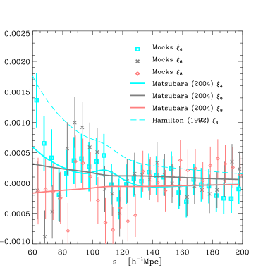
Figure 10: Mean high order multipoles from the set of 160 LasDamas mock catalogues compared with linear theory predictions based on Hamilton (1992) (dashed line) and Matsubara (2004) (solid lines). The variances correspond to the uncertainty in the mean measurements. Large angle effects (which are included in the formulae of Matsubara, 2004) reduce the amplitude of $\xi_{4}$ and cause the apparent $\xi_{6}$, $\xi_{8}$ results.

To predict how well the ongoing BOSS survey will do, we analyse mock galaxies of the volume and number density expected for this sample. Although we predict improvements in constraining $H$ by using information on $\xi_{4}$, this assumes both measuring a signal and being able to model it. In practice, BOSS should yield low S/N at  baryonic acoustic feature scales, meaning that the use of $\xi_{4}$ would only be possible at smaller scales, where velocity-dispersion effects which are difficult to model are more important.

Because we test for only a few types of 1D projections, there is room for further investigation for an optimal statistic for extracting cosmological information from clustering through the  AP test. Nonetheless, having various types of statistics yielding consistent results provides an important tool to test for systematics.

We suggest that a Fisher Matrix analysis could serve as an analytic method to test for an optimal method, to be followed up with mock catalogue tests.

Once the above are achieved, Figure 2 demonstrates that degeneracies between $\Omega_{\rm M0}$, $\Omega_{\rm K}$ and the dark energy equation of state $w$ within the $H-\,D_{\rm A}$ plane may be resolved by using clustering at high redshifts ($z>2$; e.g, through Lyman-$\alpha$ forest, and 21 cm measurements) in a complementary fashion to other observations (e.g, the temperature fluctuations of the CMB). At lower redshifts the degeneracies between these parameters is quite large at a single redshift, but might be resolved by measuring $H(z)$ at various redshifts.

In the coming years a variety of new large volume galaxy surveys will measure the large-scale clustering pattern of the Universe with unprecedented precision. Investigations of techniques such as the reconstruction of the  baryonic acoustic feature (Eisenstein et al. 2007; Seo et al. 2010; Mehta et al. 2011, Padmanabhan et al (in prep.)) suggest possible substantial improvements on constraining the cosmic evolution out of the information from these surveys and hence on our understanding of dark energy. That said, these measurements will always be bound to the  AP effect. The 1D clustering projection techniques discussed here will be essential to ensure that the full potential of the information contained in the  AP effect will be realised.

Appendix A Hexadecapole terms

In §3.4 we give analytic expressions for the  AP effect on the monopole and quadrupole. Here we extend this treatment to take into account the hexadecapole $\xi_{4}$ contribution. In this case Equation (20) becomes:

$$\xi^{\mathcal{D}}_{2}(s)=\xi_{2}(\alpha s)+\epsilon\left(2\frac{d\xi_{0}(s)}{d\ln(s)}+\frac{6}{7}\xi_{2}(\alpha s)+\frac{4}{7}\frac{d\xi_{2}(s)}{d\ln(s)}+\frac{20}{7}\xi_{4}(\alpha s)+\frac{4}{7}\frac{d\xi_{4}(s)}{d\ln(s)}\right).$$ (28)

In our analyses of the  AP effect on the $\xi_{2}$ measurement from the mock catalogues, we find the $\xi_{4}$ and d$\xi_{4}/$d$\ln s$ corrections negligible. Limiting the hexadecapole to $\ell<=4$ contributions we obtain:

$$\xi^{\mathcal{D}}_{4}(s)=\xi_{4}(\alpha s)+\epsilon\left(\frac{36}{35}\frac{d\xi_{2}(s)}{d\ln(s)}-\frac{10}{77}\xi_{4}(\alpha s)+\frac{115}{154}\frac{d\xi_{4}(s)}{d\ln(s)}\right),$$ (29)

where a higher $\ell$ would be required for completeness.

Appendix B Testing wedge widths and intermixing terms

In Figure 11 we explore the effectiveness of the wedge correction terms ${\mathcal{C}}_{||,\perp}$ (Equation 23). These results should be compared to those shown in the bottom plots of Figure 4, The short-dashed blue lines are the $2\sigma$ results shown in Figure 4, meaning when including ${\mathcal{C}}_{||,\perp}$ terms. The thick single-dot-dashed black lines are the $2\sigma$ results from the same tests where we set ${\mathcal{C}}_{||,\perp}=0$. Two interesting differences are apparent. The most obvious one is the small bias relative to the true cosmology which produces a shift in the contour lines (although within the $1\sigma$ region). Interestingly, our second observation is that it yields apparently tighter constraints than the corrected method (colored contour). These observations are noticeable in both spaces.

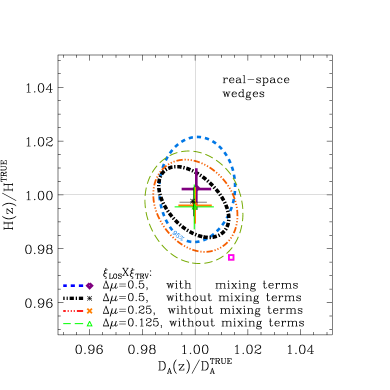
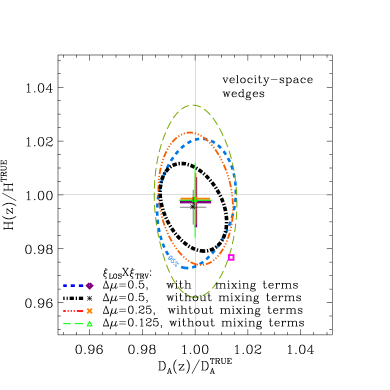
Figure 11: Joint $2\sigma$ constraints on the $H-\,D_{\rm A}$ plane obtained when analyzing the  AP effect for various clustering widths $\Delta\mu$ in real-space (upper panel) and velocity-space (lower panel). For $\Delta\mu=0.5$ we test the effect of the correciton terms ${\mathcal{C}}_{||,\perp}$ (short-dashed blue; same results as in Figure 4) and without (thick dot-dashed black; ${\mathcal{C}}_{||,\perp}=0$). (Ignoring intermixing terms means $\xi_{||}$ depends solely on $H$ and $\xi_{\perp}$ on $\,D_{\rm A}$.) As indicated in the legend for each statistic, the symbols are the most likely 2D values, and the crosses show the marginalized $1\sigma$ results. We see that not including ${\mathcal{C}}_{||,\perp}$ biases the results, and underestimates uncertainties. We also show results for analyses of thinner wedges of $\Delta\mu=0.25,\ 0.125$ (as indicated in legend). For these results we do not use correction terms in the analysis. We notice a clear trend of less bias as $\Delta\mu$ decreases, which is expected as the intermixing terms are less important. The increase in uncertainty reflects the fact that we are using less information. In velocity-space this is seen very sharply by the elongation along the $H$ direction.

In Figure 11 we also investigate other choices of radial and transverse wedges and give $2\sigma$ results for: $\Delta\mu=0.125$ and $0.25$, where we do not use correction terms (i.e, ${\mathcal{C}}_{||,\perp}$=0).

Our results clearly show, as expected, that using more information, i.e., through wider wedges yields tighter constraints. We also notice that decreasing $\Delta\mu$ reduces the bias in the obtained constraints on $\,D_{\rm A}$ both in real- and velocity-space. In velocity-space the bias is improved also in the $H$ direction. We have not investigated the constraining power of multiple thin wedges, but rather that of the two extermes $\mu>\Delta\mu$ and $\mu<\Delta\mu$.

In both spaces we notice that the narrower clustering wedges yield contours with reduced correlation coefficients between parameters $H$ and $\,D_{\rm A}$. This is expected due to weaker intermixing terms with decreasing $\Delta\mu$. This is most prominent in velocity-space where the contours sharpen towards the line-of-sight. In real-space the ellipticity appears to decreas with $\Delta\mu$.

Appendix C Proof of Concept: using Analytic Predictions

Here we demonstrate the applicability of Equations (19)–(23) to reproduce the distortions in the various multipoles and clustering wedges introduced by the use of an incorrect cosmology when transforming the observed redshifts to distances. For this we use the formulae of Matsubara (2004) for the velocity-space $\xi(\mu,s)$. We use their equation 1 which yields the two-point correlation function $\xi(z_{1},z_{2},\gamma)$ for pairs of objects located at redshifts $z_{1}$ and $z_{2}$ separated by observer angle $\gamma$. Applying Equation (3), and basic Euclidean comoving geometry, we project this result around $z_{1}$ to obtain a $\xi(\mu,s)$ plane, where the line-of-sight direction is defined as the bisecting vector from the observer to $\vec{s}$ (i.e., the same as we do with the mock catalogues). We then project $\xi(\mu,s)$ into the various multipole and wedge components.

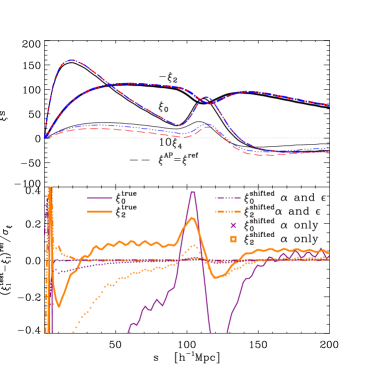
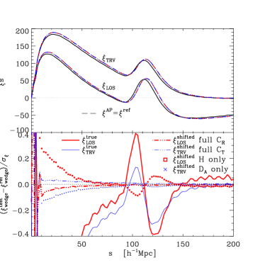
Figure 12: Analytical velocity-space clustering projections (based on Matsubara 2004) with and without the  AP effect. Left: multipoles (corresponding to Equations 19, 20). Right: $\Delta\mu=1/2$ wedges (Equations 21-23). In the top panel of each plot are the 1D projections, and in the bottom panels the difference of each result with the DISTORTED signal (labeled as AP) normalized by the uncertainty of one realization. As indicated in legend, solid lines are the true projection signals ($\,{\mathcal{T}}$), the long-dashed lines are the AP signals ($\,{\mathcal{D}}$). We apply the AP shift on true signals to obtain the triple-dot-dashed lines ($\,{\mathcal{S}}$). A perfect shift would yield a null result in the bottom panels. The symbols represent applying only zeroth order corrections. For multipoles this means applying only isotropic dilation correction ($\alpha$) and no warping terms ($\epsilon$). We see that the warping is crucial for correcting $\xi_{2}$ but negligible (although visible here) for the monopole. For the wedges zeroth order means applying only $H$ ratio corrections for radial wedge, and applying $\,D_{\rm A}$ ratio for transverse (meaning no ${\mathcal{C}}_{||,\perp}$ corrections). The  AP distortion applied here is using $w^{\rm FID}=-1.1$ instead of the true value $-1$ when converting $z$ to comoving distances.

For the true signal $\xi^{\,{\mathcal{T}}}$ $\xi$ we use the true input $P(k)$ cosmology in Equation (3). For the distorted signal $\xi^{\,{\mathcal{D}}}$ we apply the  AP effect in which we apply the same exact procedure, except that in Equation (3) we assume an equation of state $w=-1.1$ instead of the true $-1$ value. For the shifted signal $\xi^{\,{\mathcal{S}}}$ we apply the scaling given by Equations (19) and (20) on the $\xi^{\,{\mathcal{T}}}$ signal of the monopole, quadrupole pair (and also on $\xi_{4}$), and Equations (21), (22), and (23) for the $\Delta\mu=0.5$ wedges.

Our results are shown in the upper panels of Figure 12 for the multipoles (left) and clustering wedges (panels), rescaled by $s^{2}$ for clarity. The bottom panels compare the predictions of Equations (19)–(23) with the $\xi^{\,{\mathcal{D}}}$ (or $\xi^{\rm AP}$) results. A perfect description of the  AP effect would result in zero values along the solid line. By comparing results of $(\xi^{\,{\mathcal{S}}}_{\rm stat}-\xi^{\rm AP}_{\rm stat})/\sigma_{\xi_{\rm stat}}$ and $(\xi^{\,{\mathcal{T}}}_{\rm stat}-\xi^{\rm AP}_{\rm stat})/\sigma_{\xi_{\rm stat}}$ we verify that Equations (19)–(23) accuratedly describe the  AP effect and can be used to correct for it. Here “stat” means the various 1D statistics investigated: $\xi_{0,2,||,\perp}$.

We also examine the importance of the first order $\epsilon$ correction in each projection relative to the zeroth order. In the multipoles the zeroth order term is defined as applying only the isotropic dilation parameter $\alpha$, meaning assuming $\xi_{\ell}^{\mathcal{D}}(s)=\xi_{\ell}(\alpha s)$. In the wedges the zeroth order means applying only the $H$ ratio in the radial, and $\,D_{\rm A}$ in the transverse. This means assuming ${\mathcal{C}}_{||,\perp}=0$ in Equations (21) and (22) for $\Delta\mu=1/2$.

The first order correction in all projections is defined here by adding the warping term $\epsilon$ which include derivatives of the projections.

The improvement in the monopole is subtle, and negligible for any practical case. In $\xi_{2}$ the $\epsilon$ term is, of course, essential for describing the  AP shift. In the $\Delta\mu=0.5$ wedges, interestingly, the first order corrections yield slightly better results, meaning that the radial wedge is most sensitive to $H$ and the transverse on $\,D_{\rm A}$. In Appendix B we show, using mock catalogues, that the ${\mathcal{C}}(\epsilon)$ intermixing terms are essential to use in the wedge  AP correction technique to yield unbiassed $H,\ \,D_{\rm A}$ results, and that without them the uncertainties in these parameters are underestimated.

Appendix D Projections in practice: relating wedges to multipoles

In Figure 13 we put Equation (11) to the test both analytically and using mock galaxy catalogues by comparing $\Delta\mu=0.5$ wedges which are calculated directly to those approximated by the multipoles.

All uncertainty bars in the mocks are for the mock mean. All results (analytical and mocks) assume measurements of galaxies at $\langle{z}\rangle\sim 0.33$ with a bias of $b\sim 2$ with the same flat $\Lambda$CDM cosmology.

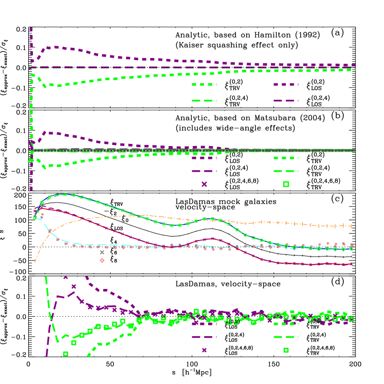
Figure 13: Panels (a),(b),(d) show the difference between clustering wedges inferred from multipoles ($\xi^{([\ell])}$), $\xi_{\rm wedge}^{\rm approx}$, and those calculated directly, $\xi_{\rm wedge}^{\rm exact}$, normalized by the uncertainty of one mock realization. $\xi_{\rm wedge}^{([\ell])}$ indicates the multipoles [$\ell$] used in the approximation. Panel (a) show results for analytic formulae in Hamilton (1992), and (b) Matsubara (2004), respectively. Including the contribution from higher order multipoles improves the results with respect to those obtained when only the monopole-quadrupole pair is used. Panels (c),(d) show similar results for the LasDamas mock catalogues, where (c) shows the actual statistics. At large scales, $\xi_{0}$ and $\xi_{2}$ are sufficient to accurately describe clustering wedges obtained from the mock catalogues, and higher order multipoles are required for $s<30$ $h^{-1}$Mpc.

D.1 Relating multipoles and wedges: analytic treatment

In this section we test the relation between the clustering wedges and the multipoles by using theoretical predictions for $\xi(\mu,s)$. For this we use the prescriptions of Hamilton (1992) (Figure 13a) and Matsubara (2004) (Figure 13b). Both of these formalisms take into account only the Kaiser squashing effect in the plane-parallel approximation (and no velocity-dispersion), but the latter also includes wide-angle effects as well as linear growth evolution between points $z_{1}$ and $z_{2}$ (see Appendix C for a brief explanation on manipulations of Equation 1 of Matsubara 2004). For the Hamilton (1992) prescription we calculate $\xi_{0}$, $\xi_{2}$, and $\xi_{4}$ directly by using their Equations 6-8, where the matter correlation function is calculated from the output of CAMB (Lewis et al. 2002). For the formulae of Matsubara (2004) we use the same matter $\xi(r)$ to compute $\xi(\mu,s)$, and integrate to obtain multipoles using Equation (8). In each case, the “directly” calculated wedges are computed by integrating $\xi(\mu,s)$, and defining the radial $\xi_{\rm\parallel}$ as $\mu>0.5$ and transverse $\xi_{\rm\perp}$ as $\mu<0.5$.

To calculate the “approximated” clustering wedges $\xi_{\rm Wedge}^{(0,2)}$, that is, only taking into account the monopole and quadrupole contributions, we use Equation (11). When adding the term of the hexadecapole $\xi_{\rm Wedge}^{(0,2,4)}$, we add the contribution of Equation (10). When using the formulae of Matsubara (2004) (panel b) we also calculate $\xi_{\rm Wedge}^{(0,2,4,6,8)}$ by following a similar procedure using $\xi_{6}$ and $\xi_{8}$. Results are given in terms of $(\xi_{\rm wedge}^{\rm true}-\xi_{\rm wedge}^{\rm approximated})/\sigma_{\xi}$, where $\sigma_{\xi}$ corresponds to the $\sqrt{C_{ii}}$ obained from the $0.16<z<0.44$ LasDamas mocks.

Due to the fact that according to the prescription of Hamilton (1992) $\xi(\mu,s)$ contains contributions only from even multipoles up to the hexadecapole, this $\ell=4$ contribution is critical for an absolute definition of the wedges. By neglecting this term the wedge approximations $\xi_{\rm Wedge}^{(0,2)}$ are inaccurate at the $\sim 1.5\%$ level (in terms of fractions $\xi^{\rm approx}/\xi^{\rm exact}$) at the barionic acoustic feature, which corresponds to $4\%$ of $\sigma_{\xi}$.

For the formulae of Matsubara (2004) we follow a similar procedure, where we also note contribution due to higher multipoles. We notice improvement from $\xi_{\rm Wedge}^{(0,2)}$ to $\xi_{\rm Wedge}^{(0,2,4)}$ and even further improvement with $\xi_{\rm Wedge}^{(0,2,4,6,8)}$. The $\xi_{6},\ \xi_{8}$ contributions are not expected from the linear squashing effect, but rather are a result of wide observer angle effects. We verify that $\xi_{6}$ and $\xi_{8}$ vanish when running the algorithm at $z=3$.

Comparing the results for $\xi_{\rm wedges}^{(0,2)}$ obtained using the prescription of Matsubara (2004) to those from the recipe of Hamilton (1992), we note that the former asymptots to zero faster. This can be explained by the fact that the $\xi_{4}$ term in Matsubara (2004) is suppressed due to the rise of higher order terms. This is clearly seen in Figure 10 where $\xi_{6}$ is comparable to $\xi_{4}$ at the  baryonic acoustic feature and surpasses it at larger scales and $\xi_{8}$ is comparable to $\xi_{4}$ at $s>130$ $h^{-1}$Mpc.

To conclude, these tests show that the clustering wedges can be accuratedly described in terms of the multipoles, and hence can be used as an alternative basis.

D.2 Analysis of mock catalogues

Here we perform a similar analysis as in the previous section but using the results for the mean multipoles and wedges obtained from the $160$ LasDamas mock catalogues described in §2.2 in real-space and velocity-space. As these include velocity-dispersion effects, as well as the expected wide-angle effects, we study even multipoles up to the eighth order. In practice, here all clustering multipoles and wedges are estimated by integrating $\xi(\mu,s)$ which is calculated with the Landy & Szalay (1993) estimator. In Appendix E we discuss an alternative approach to calculating these 1D statistics.

We find that the monopole and quadrupole approximations $\xi_{\rm Wedge}^{(0,2)}$ appear to be sufficient to describe the clustering wedges on all scales in real-space. In velocity-space they appear to be sufficient for scales $s>70$ $h^{-1}$Mpc, as seen as thick short dashed lines in Figure 13c,d. In real-space, of course, the only term is the monopole, but we do obtain higher order multipoles resulting from noise, and on large scales from angular effects. In velocity-space adding even multipoles $\ell>2$ improves results at $s<70$ $h^{-1}$Mpc. These $\ell>2$ terms appear due to velocity-dispersion effects on large scales and dominate at $s>30$ $h^{-1}$Mpc(Scoccimarro, 2004).

In Figure 10 we focus on the mock $\ell=4,6,8$ multipoles, where uncertainties are for the mock mean of $160$ realizations. These are compared to those analytically obtained from Hamilton (1992) ($\xi_{4}$ only: dashed line) and Matsubara (2004) (solid lines). The mock $\xi_{4}$ result appears to have structure similar to that expected according to Matsubara (2004) (that is, inclulding wide-angle effects). We might be seeing a  baryonic acoustic feature at $\sim 100$ $h^{-1}$Mpc. Although the large uncertainties indicate low significance, we note that similar real-space analysis yields a negative $\xi_{4}$ (but consistant with zero at a level of $2\sigma$), indicating that the velocity-space result is not due to angular effects only. Figure 11 in Samushia et al. (2011) shows similar trends in the mock $\xi_{4}$.

We conclude that the two wide clustering wedges ($\Delta\mu=0.5$) are defined fairly well by the monopole and quadrupole in velocity-space (and monopole only in real-space), and hence may be used as a alternative basis to these multipoles to project most of the information contained in $\xi(\mu,s)$.

Appendix E $\xi$ Estimators

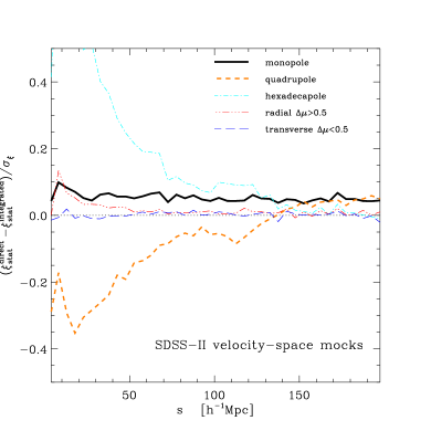
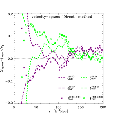
Figure 14: The left panel shows differences between the statistics obtained when using the “direct” method ($\xi^{\rm direct}$; 1D binning in pair-counter) and the “integrated” method ($\xi^{\rm integrated}$; integrating over 2D binning) in units of $\sigma_{\xi}$. Differences arrise due to wide angle effects for these clustering scales at $\langle{z}\rangle=0.33$. We clearly see that the wide wedges are the least affected. The right panel shows the relationship between the difference between the actual $\Delta\mu=0.5$ clustering wedges to those statistics approximated when using multipole combinations $\xi^{[\ell]}$ (Equation 6) in units of $\sigma_{\xi}$. In all cases shown here we use the “direct” measurements, while in Figure 13d we show a simliar comparison for $\xi^{\rm integrated}$. We clearly see that the latter test is more successful, indicating the “integrated” method to be a more natural technique.

For our $\xi$ analysis of the mocks we have used the Landy & Szalay (1993) estimator which has been shown in various studies as the lowest variance known (e.g, Kerscher et al. 2000; Kazin et al. 2010a). We examine two methods in which the 1D $\xi_{\ell}$ multipole and wedge statistics can be calculated:

1. “Integrated”: calculating $\xi(\mu,s)$ in 2D bins and integrating using Equation 7 for the multipoles and Equation 6 for the wedges.

2. “Direct”: calculating the statistics in 1D bins directly in the pair-counter.

For the “direct” method the 1D estimators can be generically written as:

$$\hat{\xi}^{\rm direct}_{\ell}(s)=\frac{DD_{\rm stat}(s)+RR_{\rm stat}(s)-2\cdot DR_{\rm stat}(s)}{RR_{\rm projection\ type}(s)}.$$ (30)

The $DD,\ RR,\ DR$ are the usual normalized data-data, random-random, data-random pair counts. By normalized we refer to the fact that it is common to reduce shot-noise effects of the random points by assigning many more random points $N_{\rm R}$ than data $N_{\rm D}$: $r\equiv N_{\rm R}/N_{\rm D}\gg 1$. This means, that when one counts number of data-data points $N_{\rm dd}$ the estimator requires it to be normalized to the random-random $N_{\rm rr}$ by $DD\equiv N_{\rm dd}\cdot r^{2}$, while for data-random this is $DR\equiv N_{\rm dr}\cdot r$.

The “stat” subscript indicates the required weighting for each statistic. For the multipoles stat$=\ell$, meaning the weight is the $\ell$ Legendre polynomials ${\mathcal{P}}_{\ell}(\mu)$. Technically this means when counting data-random pairs of the multipole $N^{\ell}_{\rm dr}(s)$, e.g, it is increased by: $N_{\rm dr}^{\ell}+=w_{\rm d}\cdot w_{\rm r}\cdot{\mathcal{P}}_{\ell}(\mu)$, if a pair is within range of $[s-0.5\Delta s,s+0.5\Delta s]$ and has a $\mu$ within $[\mu-0.5\Delta\mu,\mu+0.5\Delta\mu]$. The weights $w_{i}$ could be due to incompleteness in uniformity (angular or radial), otherwise they are unity. For the multipoles the denominator term is that of the monopole, meaning $RR_{\rm multipoles}=RR_{0}$.

The wedge estimators are similar in the nominator, but the denominator is different. For example, data-random pairs $N_{\rm dr}^{\rm wedge}$ for clustering wedge $\mu_{\rm min}<\mu<\mu_{\rm max}$ is increased by $w_{\rm d}\cdot w_{\rm r}$ given a pair in the separation range $[s-\Delta/2s,s+\Delta s/2]$ and within the wedge $\mu$ range, and zero contribution otherwise. Because the nominator “weighting” is that of a top hat, the denominator term $RR_{\rm wedge}$ in the same as in the nominator.

In this study we focused on two wide $\Delta\mu=0.5$ wedges, but this can, of course, be generalized to finer widths. One simple sanity check for $\Delta\mu=0.5$ wedges is to verify that the average of both wedges yields the monopole.

These two methods (“direct” and “integrated”) should yield a similar result given $RR$ is not a function of $\mu$, but only of separation $s$. If this is the case, the “direct” method should be preferred because the “integrated” yields lower S/N due to binning effects.

Samushia et al. (2011) point out, however, both wide angle effects as well as observer angle effects on the current SDSS-II geometry. When analyzing $RR(\mu,s)$ of the LasDamas SDSS-II mocks, we find a $\sim 10\%$ of $1\sigma$ difference between $RR(1,s)$ to $RR(0,s)$ for the  baryonic acoustic feature scale, indicating the survey is wider than it is broader. In the BOSS $0.16<z<0.6$ mocks we obtain similar conclusions only this time a $\sim 5\%$ of $1\sigma$ effect. In this case, by using the “direct” method (Equation 30), one is introducing an angular weighting of $RR(\mu,s)/RR_{0}(s)$ such that the $RR(\mu,s)$ is disregarded. In other words, Equation (30) is not equal to Equation (8). For example, the “direct” multipoles actually take the form:

$${\hat{\xi}_{\ell}(s)=\frac{DD_{\ell}(s)+RR_{\ell}(s)-2DR_{\ell}(s)}{RR_{0}(s)}}=\frac{2\ell+1}{2}\int_{-1}^{+1}{\rm d}\mu\frac{DD(\mu,s)+RR(\mu,s)-2DR(\mu,s)}{RR(\mu,s)}{\mathcal{P}}_{\ell}(\mu)\cdot\frac{RR(\mu,s)}{RR(s)}.$$ (31)

In the left panel of Figure 14 we show the difference between the two methods for clustering $\xi_{0,2,4}$ and $\Delta\mu=0.5$ wedges. The difference between “direct” and “integrated” is given in units of $\sigma_{\xi}$ for the SDSS-II mocks.

We clearly see an over estimation of the “direct” results in most scales for the multipoles. At the  baryonic acoustic feature scale this effect in units of $1\sigma$ is $\sim 5\%$ for $\xi_{0}$, $\sim 7\%$ for $\xi_{2}$ and $\sim 8\%$ for $\xi_{4}$, with the differences for the last two cases increasing at smaller scales. We note that the uncertainties of $\xi_{2}$ and $\xi_{4}$ are much larger than that of $\xi_{0}$ making the ratios $\xi^{\rm direct}_{\ell}/\xi^{\rm integrated}_{\ell}$ larger than that of the monopole.

The $\Delta\mu=0.5$ wedges, on the other hand, are shown to yield much smaller differences. This is probably due to the fact that the wide wedges do not correlate pairs at $\mu=0$ with those at $\mu=1$.

Another comparison is shown on the right panel of Figure 14 which is similar to that in Figure 13d. As described in Appendix D, both test the relation between clustering wedges and multipoles (Equation 11), where the right panel of Figure 14 corresponds to the “direct” method, and Figure 13d shows the “integrated” measurements. We clearly see that the “integrated” method performs better.

Although the “integrated” estimator method appears to be closer to the natural definition of multipoles and wedges, there is a tradeoff of increase in uncertainties due to binning effects (one is integrating of more noisy $DD$). Also, by using the “integrated” method explained here, one might be adding observer angle effects discussed in Samushia et al. (2011). For this reason, we conclude that the user should be aware of the two methods, and choose accordingly. We recommend applying both and comparing the obtained results. The “direct” method might be preferable if the user ads the $RR(\mu,s)/RR_{0}(s)$ weighting into the multipole $\xi_{\ell}$ model. For the $\Delta\mu=0.5$ wedges we show no substantial difference in the actual $\xi$, so one would choose the one that yields lower uncertainties.

References

- Alcock & Paczynski (1979) Alcock, C. & Paczynski, B. 1979, Nature, 281, 358
- Arnalte-Mur et al. (2011) Arnalte-Mur, P., Labatie, A., Clerc, N., Martínez, V. J., Starck, J., Lachièze-Rey, M., Saar, E., & Paredes, S. 2011, ArXiv e-prints
- Ballinger et al. (1996) Ballinger, W. E., Peacock, J. A., & Heavens, A. F. 1996, MNRAS, 282, 877
- Berlind & Weinberg (2002) Berlind, A. A. & Weinberg, D. H. 2002, ApJ, 575, 587
- Blake et al. (2011) Blake, C., Brough, S., Colless, M., Contreras, C., Couch, W., Croom, S., Davis, T., Drinkwater, M. J., Forster, K., Gilbank, D., Gladders, M., Glazebrook, K., Jelliffe, B., Jurek, R. J., Li, I., Madore, B., Martin, C., Pimbblet, K., Poole, G., Pracy, M., Sharp, R., Wisnioski, E., Woods, D., Wyder, T., & Yee, H. 2011, ArXiv e-prints
- Blake et al. (2007) Blake, C., Collister, A., Bridle, S., & Lahav, O. 2007, MNRAS, 374, 1527
- Blake & Glazebrook (2003) Blake, C. & Glazebrook, K. 2003, ApJ, 594, 665
- Cabré & Gaztañaga (2009) Cabré, A. & Gaztañaga, E. 2009, MNRAS, 393, 1183
- Cole et al. (2005) Cole, S., Percival, W. J., Peacock, J. A., Norberg, P., Baugh, C. M., Frenk, C. S., Baldry, I., Bland-Hawthorn, J., Bridges, T., Cannon, R., Colless, M., Collins, C., Couch, W., Cross, N. J. G., Dalton, G., Eke, V. R., De Propris, R., Driver, S. P., Efstathiou, G., Ellis, R. S., Glazebrook, K., Jackson, C., Jenkins, A., Lahav, O., Lewis, I., Lumsden, S., Maddox, S., Madgwick, D., Peterson, B. A., Sutherland, W., & Taylor, K. 2005, MNRAS, 362, 505
- Colless et al. (2003) Colless, M., Peterson, B. A., Jackson, C., Peacock, J. A., Cole, S., Norberg, P., Baldry, I. K., Baugh, C. M., Bland-Hawthorn, J., Bridges, T., Cannon, R., Collins, C., Couch, W., Cross, N., Dalton, G., De Propris, R., Driver, S. P., Efstathiou, G., Ellis, R. S., Frenk, C. S., Glazebrook, K., Lahav, O., Lewis, I., Lumsden, S., Maddox, S., Madgwick, D., Sutherland, W., & Taylor, K. 2003, ArXiv Astrophysics e-prints
- Crocce & Scoccimarro (2008) Crocce, M. & Scoccimarro, R. 2008, Phys. Rev. D, 77, 023533
- Crocce et al. (2011) Crocce, M., Gaztanaga, E., Cabre, A., Carnero, A., & Sanchez, E. 2011, ArXiv e-prints
- Dalal et al. (2008) Dalal, N., Doré, O., Huterer, D., & Shirokov, A. 2008, Phys. Rev. D, 77, 123514
- Drinkwater et al. (2010) Drinkwater, M. J., Jurek, R. J., Blake, C., Woods, D., Pimbblet, K. A., Glazebrook, K., Sharp, R., Pracy, M. B., Brough, S., Colless, M., Couch, W. J., Croom, S. M., Davis, T. M., Forbes, D., Forster, K., Gilbank, D. G., Gladders, M., Jelliffe, B., Jones, N., Li, I., Madore, B., Martin, D. C., Poole, G. B., Small, T., Wisnioski, E., Wyder, T., & Yee, H. K. C. 2010, MNRAS, 401, 1429
- Eisenstein & Hu (1998) Eisenstein, D. J. & Hu, W. 1998, ApJ, 496, 605
- Eisenstein et al. (1998) Eisenstein, D. J., Hu, W., & Tegmark, M. 1998, ApJ, 504, L57+
- Eisenstein et al. (1999) Eisenstein, D. J., Hu, W., & Tegmark, M. 1999, ApJ, 518, 2
- Eisenstein et al. (2005) Eisenstein, D. J. et al. 2005, ApJ, 633, 560
- Eisenstein et al. (2007) Eisenstein, D. J., Seo, H.-J., Sirko, E., & Spergel, D. N. 2007, ApJ, 664, 675
- Eisenstein et al. (2011) Eisenstein, D. J., Weinberg, D. H., Agol, E., Aihara, H., Allende Prieto, C., Anderson, S. F., Arns, J. A., Aubourg, E., Bailey, S., Balbinot, E., & et al. 2011, ArXiv e-prints
- Estrada et al. (2009) Estrada, J., Sefusatti, E., & Frieman, J. A. 2009, ApJ, 692, 265
- Friedman (1922) Friedman, A. 1922, Zeitschrift fur Physik, 10, 377
- Fry (1996) Fry, J. N. 1996, ApJ, 461, L65+
- Gaztañaga et al. (2009) Gaztañaga, E., Cabré, A., & Hui, L. 2009, MNRAS, 399, 1663
- Glazebrook & Blake (2005) Glazebrook, K. & Blake, C. 2005, ApJ, 631, 1
- Hamilton (1992) Hamilton, A. 1992, ApJ, 385, L5
- Hamilton (1998) Hamilton, A. J. S. 1998, in Astrophysics and Space Science Library, Vol. 231, The Evolving Universe, ed. D. Hamilton, 185–+
- Hogg (1999) Hogg, D. W. 1999, astro-ph/9905116
- Hu & Haiman (2003) Hu, W. & Haiman, Z. 2003, Phys. Rev. D, 68, 063004
- Hubble & Humason (1931) Hubble, E. & Humason, M. L. 1931, ApJ, 74, 43
- Hui et al. (2007) Hui, L., Gaztañaga, E., & Loverde, M. 2007, Phys. Rev. D, 76, 103502
- Hütsi (2006) Hütsi, G. 2006, A&A, 449, 891
- Jackson (1972) Jackson, J. C. 1972, MNRAS, 156, 1P
- Jones et al. (2009) Jones, D. H., Read, M. A., Saunders, W., Colless, M., Jarrett, T., Parker, Q. A., Fairall, A. P., Mauch, T., Sadler, E. M., Watson, F. G., Burton, D., Campbell, L. A., Cass, P., Croom, S. M., Dawe, J., Fiegert, K., Frankcombe, L., Hartley, M., Huchra, J., James, D., Kirby, E., Lahav, O., Lucey, J., Mamon, G. A., Moore, L., Peterson, B. A., Prior, S., Proust, D., Russell, K., Safouris, V., Wakamatsu, K.-I., Westra, E., & Williams, M. 2009, MNRAS, 399, 683
- Kaiser (1987) Kaiser, N. 1987, MNRAS, 227, 1
- Kazin et al. (2010a) Kazin, E. A., Blanton, M. R., Scoccimarro, R., McBride, C. K., Berlind, A. A., Bahcall, N. A., Brinkmann, J., Czarapata, P., Frieman, J. A., Kent, S. M., Schneider, D. P., & Szalay, A. S. 2010a, ApJ, 710, 1444
- Kazin et al. (2010b) Kazin, E. A., Blanton, M. R., Scoccimarro, R., McBride, C. K., & Berlind, A. A. 2010b, ApJ, 719, 1032
- Kerscher et al. (2000) Kerscher, M., Szapudi, I., & Szalay, A. S. 2000, ApJ, 535, L13
- Kim et al. (2009) Kim, J., Park, C., Gott, J. R., & Dubinski, J. 2009, ApJ, 701, 1547
- Komatsu et al. (2009) Komatsu, E., Dunkley, J., Nolta, M. R., Bennett, C. L., Gold, B., Hinshaw, G., Jarosik, N., Larson, D., Limon, M., Page, L., Spergel, D. N., Halpern, M., Hill, R. S., Kogut, A., Meyer, S. S., Tucker, G. S., Weiland, J. L., Wollack, E., & Wright, E. L. 2009, The Astrophysical Journal Supplement, 180, 330
- Labini et al. (2009) Labini, F. S., Vasilyev, N. L., & Baryshev. 2009, ArXiv e-prints
- Landy & Szalay (1993) Landy, S. D. & Szalay, A. S. 1993, ApJ, 412, 64
- Lewis et al. (2002) Lewis, I. et al. 2002, MNRAS, 334, 673
- Linder (2003) Linder, E. V. 2003, Phys. Rev. D, 68, 083504
- Martinez et al. (2009) Martinez, V. J., Arnalte-Mur, P., Saar, E., de la Cruz, P., Pons-Borderia, M. J., Paredes, S., Fernandez-Soto, A., & Tempel, E. 2009, ApJ, 696
- Matsubara (2004) Matsubara, T. 2004, ApJ, 615, 573
- Mehta et al. (2011) Mehta, K. T., Seo, H., Eckel, J., Eisenstein, D. J., Metchnik, M., Pinto, P., & Xu, X. 2011, ArXiv e-prints
- Meiksin et al. (1999) Meiksin, A., White, M., & Peacock, J. A. 1999, MNRAS, 304, 851
- Norberg et al. (2009) Norberg, P., Baugh, C. M., Gaztañaga, E., & Croton, D. J. 2009, MNRAS, 396, 19
- Okumura et al. (2008) Okumura, T., Matsubara, T., Eisenstein, D. J., Kayo, I., Hikage, C., Szalay, A. S., & Schneider, D. P. 2008, ApJ, 676, 889