Locating the source of projectile fluid droplets

Abstract

The ill-posed projectile problem of finding the source height from spattered droplets of viscous fluid is a longstanding obstacle to accident reconstruction and crime scene analysis. It is widely known how to infer the impact angle of droplets on a surface from the elongation of their impact profiles. However, the lack of velocity information makes finding the height of the origin from the impact position and angle of individual drops not possible. From aggregate statistics of the spatter and basic equations of projectile motion, we introduce a reciprocal correlation plot that is effective when the polar launch angle is concentrated in a narrow range. The vertical coordinate depends on the orientation of the spattered surface, and equals the tangent of the impact angle for a level surface. When the horizontal plot coordinate is twice the reciprocal of the impact distance, we can infer the source height as the slope of the data points in the reciprocal correlation plot. If the distribution of launch angles is not narrow, failure of the method is evident in the lack of linear correlation. We perform a number of experimental trials, as well as numerical calculations and show that the height estimate is insensitive to aerodynamic drag. Besides its possible relevance for crime investigation, reciprocal-plot analysis of spatter may find application to volcanism and other topics and is most immediately applicable for undergraduate science and engineering students in the context of crime-scene analysis.

I Introduction

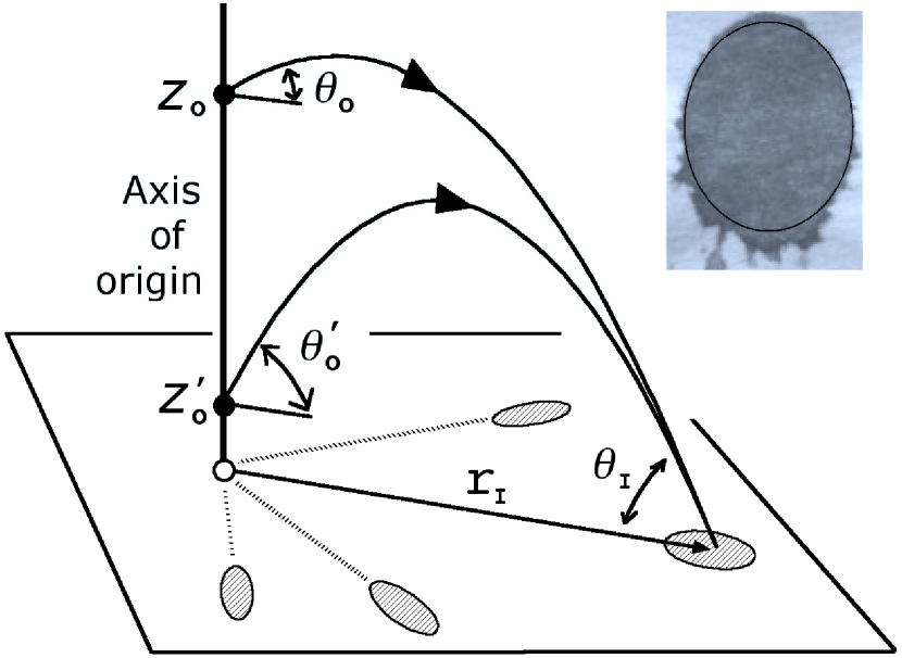
The impact of spattered droplets of viscous fluidVogel ; Leyton on a horizontal surface results in elongated impact profiles, from which it is easy to locate the vertical axis of origin from the orientation of elongated impact profiles (see Fig. 1). It is accurate for blood-like fluids (and routine practice in forensicsCarter ; Knock ) to estimate the angle of impact of a viscous droplet from its impact profile as

$$\theta_{\scriptscriptstyle{\mathrm{I}}}=\sin^{-1}\!\Big{(}\frac{\mathrm{profile\;width}}{\mathrm{length}}\Big{)}.$$ (1)

The subscript “I” denotes impact-related quantities. This construction, which assigns to each elliptical profile (see Fig. 1, inset) the projected shape of the incoming spherical droplet on the surface, works remarkably well. From estimates of $\theta_{\scriptscriptstyle{\mathrm{I}}}$ from Eq. (1) we would like to estimate the location of the droplet launch from the positions and angles of the impacts.

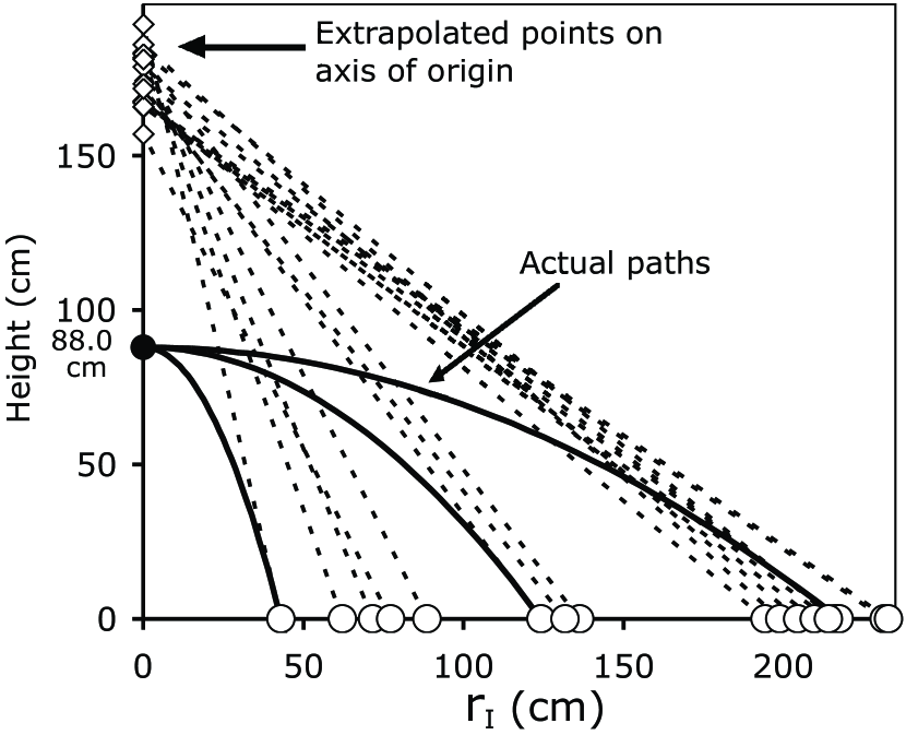
However, even when its vertical axis is known, the height of a source is not deducible from the location and impact angle of individual drops ($r_{\scriptscriptstyle{\mathrm{I}}}$ and $\theta_{\scriptscriptstyle{\mathrm{I}}}$ in Fig. 1). The impact velocity of each drop is missing the information needed to infer the source height, and thus an height must involve assumptions. A method widely used in forensicsCarter is to extrapolate straight lines from each impact back to the launch axis and seek a minimum in these height values, which is consistent only with the equations of projectile motion in the limit of high velocity and low aerodynamic drag. Otherwise, the strategy systematically overestimates the source heightCarter (see Fig. 2). Such considerations have led to alternative proposals, such as seeking missing velocity information in the detailed structure of impact profiles.Knock

In this paper we present a statistical and graphical method of back-estimation consistent with the equations of projectile motion and provide a height estimate in cases where the droplets are launched within a narrow range of the launch angle, using only the impact location and inferred impact angle. In the simplest case, linearity appears in a plot of the tangent of the impact angle versus twice the reciprocal distance of impact.

Figure 1: Profile orientations can be extrapolated (dotted lines) to a horizontal point of convergence ($\circ$) so that the vertical axis of origin and the distance $r_{\scriptscriptstyle{\mathrm{I}}}$ are known. Even with knowledge of the impact angle $\theta_{\scriptscriptstyle{\mathrm{I}}}$, we still cannot determine the source height (for example, $z_{0}$ or $z^{\prime}_{0}$). (Inset) Digitized photograph of experimental impact profile fit to an ellipse. The impact angle is obtainable from the residue profile width and length by attributing the elliptical profile to the projected shape of the incoming spherical droplet.

Figure 2: Position and impact-angle data ($\circ$) for floor spatter generated as described in Section IV (clapper horizontal; i.e. launch angle $0^{\circ}$). Extrapolated points on the axis of convergence ($\diamondsuit$) fail to estimate the source position ($\bullet$) (height $88.0\,\mathrm{cm}$) even as a lower bound (a high-velocity assumption).

Figure 3: (a) The floor spatter data of Fig. 2 in a reciprocal correlation plot, using $\tau_{\scriptscriptstyle{\mathrm{I}}}=\tan\theta_{\scriptscriptstyle{\mathrm{I}}}$ from Eq. (4). The slope yields an estimated launch height of $95.0\pm 2.2\,\mathrm{cm}$ and an estimated launch angle of $-5.8\pm 2.4^{\circ}$. Pearson’s coefficient of linear correlation is $r=0.996$. The actual source height is $88.0\,\mathrm{cm}$. (b) Trial with launch height $85.0\,\mathrm{cm}$ with the clapper sideways for a maximally broad launch angle distribution. In this case the reciprocal plot yields no height estimate, as evidenced by lack of linear correlation ($r=0.143$).

II Reciprocal plot for floor spatter

The kinematic constant-acceleration equationsSerway ; Knight for a projectile droplet in cylindrical coordinates $z$ and $r$ (neglecting aerodynamic drag) are

$$z(t)=z_{0}+\tfrac{1}{2}(v_{z}+v_{z,0})t,$$ (2)

where $z_{0}$ is the actual launch height. Along the trajectory the horizontal position is $r(t)=v_{r}t$ with $v_{r}$ the radial velocity. The vertical velocity is $v_{z}=v_{r}\tan\theta$ with $\theta$ upward from the horizontal. If we substitute $v_{z}=v_{r}\tan\theta$ and $v_{z,0}=v_{r}\tan\theta_{0}$ into Eq. (2), we find

$$\tan\theta_{\scriptscriptstyle{\mathrm{I}}}=(z_{0}-z_{\scriptscriptstyle{\mathrm{I}}})\,\frac{2}{r_{\scriptscriptstyle{\mathrm{I}}}}+\tan\theta_{0}.$$ (3)

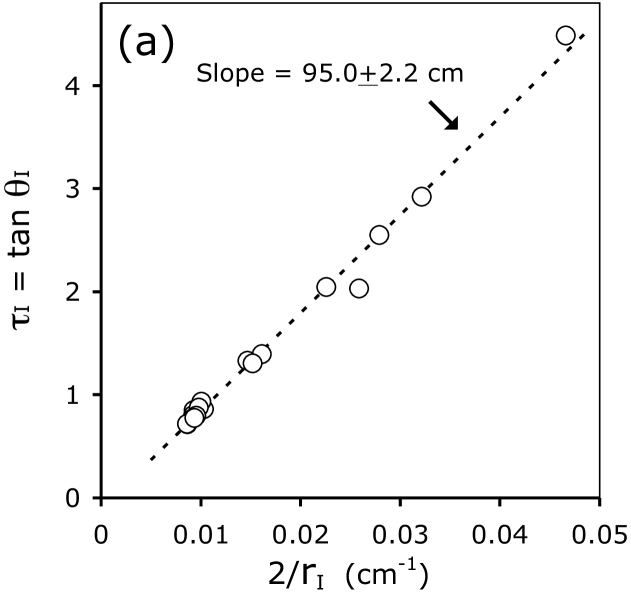
We have defined $\theta_{\scriptscriptstyle{\mathrm{I}}}$ downward (that is, as $-\theta$) so that $\theta_{\scriptscriptstyle{\mathrm{I}}}$ is positive at impact as in Fig. 1. For launch and impact at equal height ($z_{0}=z_{\scriptscriptstyle{\mathrm{I}}}$) Eq. (3) correctly predicts that $\theta_{0}=\theta_{\scriptscriptstyle{\mathrm{I}}}$. Consider impacts on a surface at $z_{\scriptscriptstyle{\mathrm{I}}}=0$ (a floor), where we have located the vertical axis of the origin (see Fig. 1) and wish to find the launch height $z_{0}$. In Fig. 3(a) we plot the quantity for actual spatter data,

$$\tau_{\scriptscriptstyle{\mathrm{I}}}({\mathrm{floor}})=\tan\theta_{\scriptscriptstyle{\mathrm{I}}}$$ (4)

versus the quantity $2/r_{\scriptscriptstyle{\mathrm{I}}}$. According to Eq. (3) our data will satisfy

$$\tau_{\scriptscriptstyle{\mathrm{I}}}=z_{0}\,\frac{2}{r_{\scriptscriptstyle{\mathrm{I}}}}+\tan\theta_{0}.$$ (5)

The slope, that is, the coefficient of $2/r_{\scriptscriptstyle{\mathrm{I}}}$, gives the launch height $z_{0}$. Figure 3(a) shows a trial using a standard “clapper” mechanism (see Sec. IV) in which a reciprocal correlation plot yields the source height as $95.0\pm 2.2$ cm compared to the actual height of 88.0 cm. The remaining discrepancy may indicate residual systematic error in our procedure, such as a surface effect on profile shape or some other factor.

Figure 4: (a) Reciprocal correlation plots for floor impacts with horizontal launch: ($\bullet$), launch height $z_{0}=88$ cm (the same data as in Fig. 2(b)); ($\circ$), launch height $z_{0}=164$ cm ($\circ$). The clapper orientation is horizontal for both trials. Note the differing slopes, due to their differing heights, but similar intercepts. (Upper curve: slope $164\pm 6$ cm, intercept $\theta_{0}=2.7\pm 3.7^{\circ}$, $r=0.996$. Lower curve as in Fig. 3(a).) (b) Plots for floor impacts, with the clapper at $\theta_{0}=45^{\circ}$ ($\bullet$) and $\theta_{0}=0^{\circ}$ ($\circ$), same data as in (a)). The heights of 165 cm and 164 cm, respectively, are similar. Note the similar slopes, but distinct intercepts. (Upper curve: slope $168\pm 4$ cm, intercept $\theta_{0}=45.8\pm 1.2^{\circ}$, and $r=0.995$. Lower curve as in part (a).)

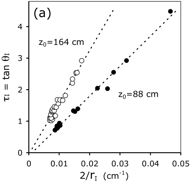
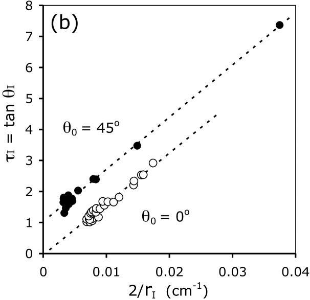
To further illustrate the predictions of Eq. (5), Fig. 4(a) shows how a varying source height above a level surface leads to different slopes in a reciprocal correlation plot. Figure 4(b) shows how varying the launch angle of spatter leads to different vertical intercepts.

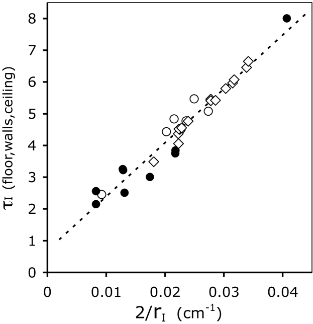
Fig. 5 applies a reciprocal plot to spatter data collected from walls and ceiling, as well as from the floor. Extensions of Eq. (4) necessary for this are discussed in Sec. IV.

Figure 5: Reciprocal correlation plot of the combined data from the floor ($\circ$), walls ($\bullet$), and ceiling ($\diamondsuit$) with $\tau_{\scriptscriptstyle{\mathrm{I}}}$ generalized as described in Sec. IV. For the combined data the slope is $z_{0}=169\pm 7\,\mathrm{cm}$ and the intercept is $35\pm 7^{\circ}$ (dotted line), compared to the actual values of $165\,\mathrm{cm}$ and $45^{\circ}$, with $r=0.973$. The separate slopes and intecepts of the floor data (height $159\pm 21\,\mathrm{cm}$ and angle $48\pm 13^{\circ}$), wall data ($167\pm 18\,\mathrm{cm}$ and $34\pm 14^{\circ}$), and ceiling data ($185\pm 14\,\mathrm{cm}$ and $14\pm 9^{\circ}$) are not statistically distinguishable.

III Aerodynamic drag

In reciprocal plots such as Figs. 3(a) and 4, points near the plot origin represent distant impacts, with high launch speed. Here an error due to aerodynamic drag might be anticipated. Our trials suggest no obvious problem, and therefore we turn to numerical calculations. The drag force on a droplet with speed $v$ isLeyton ; Batchelor ; Vogel

$$F_{d}=\frac{1}{2}\rho_{\mathrm{air}}Av^{2}\,C_{d},$$ (6)

where $A$ is the cross-sectional area, $\rho_{\mathrm{air}}$ is the density of air, and $C_{d}$ is an empirical coefficient. Separate calculations show that for our spatter trials $C_{d}\approx 0.5$. We define

$$v_{\scriptscriptstyle T} =\sqrt{\frac{4}{3}\frac{\rho_{\mathrm{liq}}}{\rho_{\mathrm{air}}}\frac{gd}{C_{d}}},$$ (7)

$$z_{\scriptscriptstyle T} =\frac{v_{\scriptscriptstyle T}^{2}}{g},$$ (8)

where $g$ is the acceleration of gravity, $v_{\scriptscriptstyle T}$ is the terminal velocity of a drop of diameter $d$ and density $\rho_{\mathrm{liq}}$, and $z_{\scriptscriptstyle T}$ is a “terminal height” over which the terminal velocity is nearly reached in a vertical fall ($v=0.93\,v_{\scriptscriptstyle T}$ at $z_{\scriptscriptstyle T}$). We write equations for the drop trajectories which incorporate Eq. (6),

$$\frac{d\tilde{v}_{x}}{d\tilde{t}} =-\tilde{v}\,\tilde{v}_{x}$$ (9a)

$$\frac{d\tilde{v}_{y}}{d\tilde{t}} =-(1+\tilde{v}\,\tilde{v}_{y})$$ (9b)

where $\tilde{v}=(\tilde{v}_{x}^{2}+\tilde{v}_{y}^{2})^{1/2}$ and we use the dimensionless variables

$$\tilde{v}_{x,y}=\frac{v_{x,y}}{v_{\scriptscriptstyle T}},\quad\tilde{r}_{\scriptscriptstyle{\mathrm{I}}}=\frac{r_{\scriptscriptstyle{\mathrm{I}}}}{z_{\scriptscriptstyle T}},\quad\tilde{t}=\frac{v_{\scriptscriptstyle T}\,t}{g}.$$ (10)

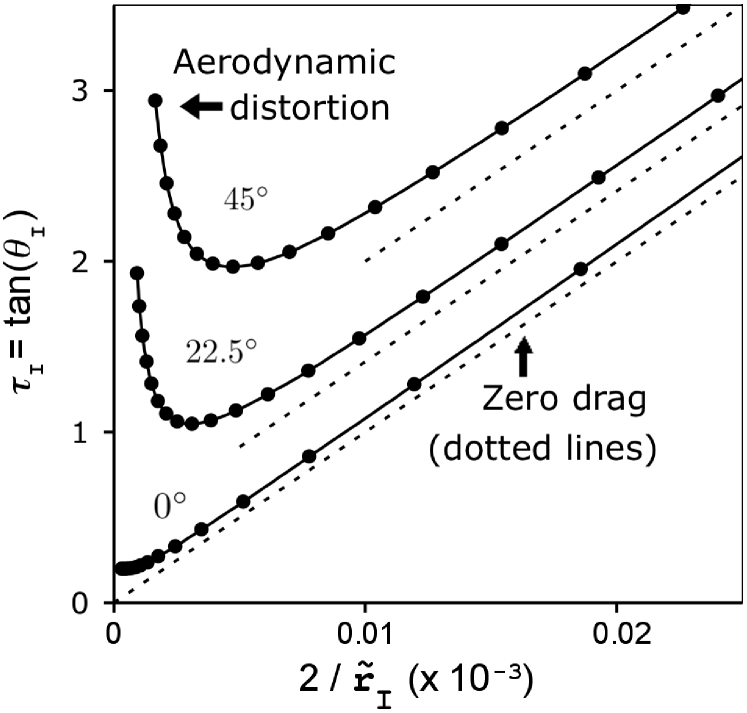
We numerically solvedPress Eq. (9) and constructed reciprocal plots in the presence of drag, at three launch angles (see Fig. 4). These dimensionless plots, rescaled to the appropriate $v_{\scriptscriptstyle T}$ and $z_{\scriptscriptstyle T}$, apply to any droplet diameter or launch height. In all cases distortion is greatest on the left side of the plot, as expected, where the range and launch speed are highest.

A notable feature of Fig. 6 is that, for moderate height and launch speed where the plot is linear, aerodynamic drag mainly affects intercepts, and thus the inferred launch angles, but not the slopes. The height of origin estimates are only weakly affected. This dependence indicates a certain robustness of the method in the presence of drag, as long as we obtain linear plots, which might help explain the success of our plots in Figs. 3(a), 4, and 5.

Figure 6: Reciprocal plots for trajectories in the presence of aerodynamic drag ($\bullet$) calculated using Eq. (9) at launch angles $0^{\circ}$, $22.5^{\circ}$, and $45^{\circ}$. The source height is $z_{0}=0.1z_{\scriptscriptstyle T}$ and $\tilde{r}_{\scriptscriptstyle{\mathrm{I}}}=r_{\scriptscriptstyle{\mathrm{I}}}/z_{\scriptscriptstyle T}$, where $z_{\scriptscriptstyle T}$ is the characteristic fall height leading to the terminal velocity. The horizontal axis is rescaled by $10^{-3}$ for rough correspondence to cm^-1 in our experiments. In the linear region the slopes are little changed from the straight lines (dotted) which would occur in the absence of drag.

IV Methods and statistics

In the spatter trials whose results are plotted in Figs. 3–5, a viscous fluid was spattered on floors, ceilings, and walls with a clapper device modeled after those used in forensics training.Carter Two wooden boards, joined at the rear by a spring-loaded door hinge, slammed shut at the front, an impact area that we fitted with metal plates. A small pouch of fluid to be spattered was taped to one plate. The results in Figs. 3(a) and 4(a) were obtained with the impact plates horizontal. To vary the launch angle we tilted the clapper forward and backward. For a broad distribution of launch angles we rotated the clapper about the long axis so that the launch area was vertically oriented.

We found that reliable impact angle estimates required considerable practice, including self-calibration using vertical drop impacts on inclined surfaces, during which we found that actual blood drops resulted in well-defined ellipses and surprisingly good impact angle estimates using Eq. (1). To avoid using actual blood in our spatter trials, we used a heterogeneous fluid whose droplet impact profiles closely resemble those of blood droplets. The majority of our experiments used approximately 2–3 parts Ashanti chicken wing sauce (Bridge Foods) with 1 part Ivory dish soap to aid cleanup, and trace amounts of food coloring to enrich the color for digitization. In other experiments, a viscous test fluid of 4 parts corn syrup to 1 part water with food coloring also led to a reasonably successful analysis.

From a typical spatter trial we chose approximately twenty profiles having well-defined elliptical profiles, representing a range of distances. For the plots, we took digital photographs of the profiles, and used image analysis softwareImageJ to manually fit the ellipses to the profile outlines shown in Fig. 1 (inset). We obtained best results by matching well-defined portions of the elliptical outline. Very close to the source, near-circular profiles can lead to large uncertainties both in Eq. (1) and in $2/r_{\scriptscriptstyle{\mathrm{I}}}$ when $r_{\scriptscriptstyle{\mathrm{I}}}$ is very small,Knock and hence some of these points were discarded.

Our estimates of slopes, intercepts, and their errors were made using standard regression techniques,Press where, for example, the estimate of the slope (that is, launch height) is

$$z_{\mathrm{est}}=z_{0}\frac{\langle{\Delta u\Delta\tau_{\scriptscriptstyle{\mathrm{I}}}}\rangle}{\langle{(\Delta u\,)^{2}}\rangle},\quad u=\frac{2z_{0}}{r_{\scriptscriptstyle{\mathrm{I}}}},$$ (11)

with $z_{0}$ equal to the actual launch height and $\Delta u=u-\langle u\rangle$, where $\langle\cdots\rangle$ denotes an average. A widely known parameter of linear correlationPress is Pearson’s $r$, which for our reciprocal plots is

$$r=\frac{\langle\Delta u\Delta\tau_{\scriptscriptstyle{\mathrm{I}}}\rangle}{\sqrt{\langle{(\Delta u)^{2}}\rangle\langle{(\Delta\tau_{\scriptscriptstyle{\mathrm{I}}})^{2}}\rangle}}.$$ (12)

A complete description of projectile motion requires that Eq. (3) be combined with the relation

$$\tan^{2}\theta_{\scriptscriptstyle{\mathrm{I}}}=(\eta^{2}\!+1)\tan^{2}\theta_{0}+\eta^{2},$$ (13)

which parameterizes lines of constant $\theta_{0}$ in the reciprocal plot by the variable $\eta=\sqrt{2gz_{0}}/v_{0}$, where $v_{0}$ is the launch speed.

Consider the special case of a product probability distribution for the launch angle and velocity $P(\theta_{0},v)=P_{1}(\theta_{0})P_{2}(v)$, where $P_{1}(\theta_{0})$ is symmetrical about the horizontal. We can obtain, using Eqs. (3), (11), (12), and (13) the simple relation

$$z_{\mathrm{est}}=r^{2}z_{0}\ \text{[for symmetric $P_{1}(\theta_{0})$]}.$$ (14)

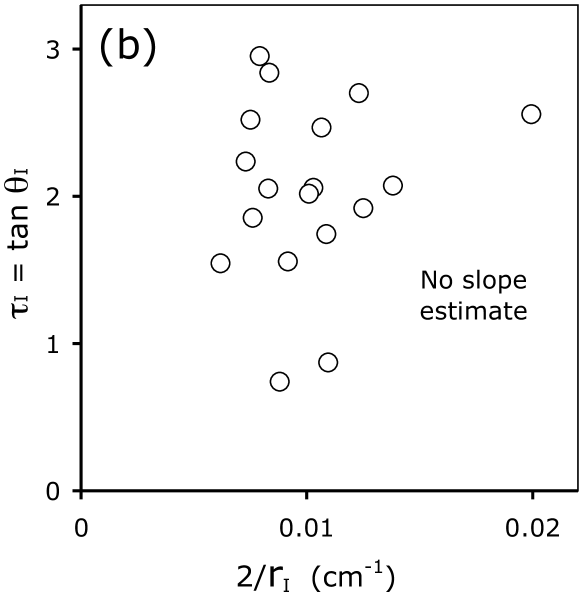
Although Eq. (14) is not general, it suggests that bias may occur in height estimates if $r^{2}$ is not reasonably close to $1$. A requirement of strong linear correlation also accords with common sense. Figure 3(b) showed an unfavorable trial in which the spread in launch angle is maximized by turning the clapper sideways. This trial was performed ten times, yielding the $r$ values $0.14$, $0.18$, $0.78$, $0.86$, $0.80$, $0.56$, $0.83$, $0.58$, $0.72$, and $0.37$. These values are all smaller than $1$, and the plots were uncorrelated in appearance. In contrast, in Figs. 3(a) and 4 $r=0.995$ or higher, and for the combined data sets in Fig. 5, $r=0.973$.

We can also combine and analyze spatter data from floors and other non-horizontal surfaces in a single reciprocal plot. Co-plotting data from non-horizontal surfaces (see Fig. 5) requires corresponding redefinitions of the variable $\tau_{\scriptscriptstyle{\mathrm{I}}}$. We then seek a slope via Eq. (5) as before. Spatter on a ceiling at height $z=z_{\scriptscriptstyle{\mathrm{I}}}$ is incorporated by adding a term to Eq. (4) and changing the sign of the tangent,

$$\tau_{\scriptscriptstyle{\mathrm{I}}}({\mathrm{ceiling}})=z_{\scriptscriptstyle{\mathrm{I}}}\frac{2}{r_{\scriptscriptstyle{\mathrm{I}}}}-\tan\theta_{\scriptscriptstyle{\mathrm{I}}}.$$ (15)

Ceiling data tended to be more robust closer to the source. On walls the right-hand side of Eq. (1) yields the angle $\theta_{\scriptscriptstyle W}$ of impact with the plane of the wall. The correct vertical angle is then $\theta_{\scriptscriptstyle{\mathrm{I}}}=\sin^{-1}\left(\cos\alpha_{\scriptscriptstyle{\mathrm{I}}}\cos\theta_{\scriptscriptstyle W}\right)$ with $\alpha_{\scriptscriptstyle{\mathrm{I}}}$ the angle from vertical of the wall profile. We plot

$$\tau_{\scriptscriptstyle{\mathrm{I}}}({\mathrm{walls}})=z_{\scriptscriptstyle{\mathrm{I}}}\frac{2}{r_{\scriptscriptstyle{\mathrm{I}}}}+\tan\theta_{\scriptscriptstyle{\mathrm{I}}},$$ (16)

where $z_{\scriptscriptstyle{\mathrm{I}}}$ is the elevation of the impact. We typically avoided near-horizontal wall impacts. Once the axis of origin is located, $\tan\theta_{\scriptscriptstyle{\mathrm{I}}}$ in Eq. (16) can be replaced by $\cos\phi_{\scriptscriptstyle{\mathrm{I}}}/\tan\alpha_{\scriptscriptstyle{\mathrm{I}}}$, where $\phi_{\scriptscriptstyle{\mathrm{I}}}$ is the angle between the wall and the vertical plane of impact, a relation which is convenient for curved vertical surfaces such as pipes.

V Discussion

We have introduced and illustrated with several experiments, a plot-based method for locating the spatial source of spattered viscous fluid. Th method is effective when the spatter is launched within a narrow range of polar angles. We showed how a reciprocal plot of the impact data, together with elementary projectile physics, can exhibit linear trends among the data points. From the slope of any strong linear correlation that occurs, we obtain a robust estimate of the height of the origin that would otherwise be unavailable. Broad distributions of launch angle cause the method to fail, and in such cases we reach a null conclusion (a lack of linear correlation), rather than an erroneous estimate of height of origin.

We also showed that the method appears insensitive to aerodynamic drag effects within some velocity regime. We also extended the plotting method to some other simple geometries.

The reciprocal plot, which is based on the correct equations of projectile motion, may eventually become a useful tool for forensic spatter analysis, where information on height of spatter origin pertains, for example, to whether a victim was sitting or standing.

Another possible use of this analysis, which we are pursuing separately, may be its application to geophysics and volcanism, especially to phenomena such as volcanic ejection and lava fountains.Wolff

The most immediate use of reciprocal-plot analysis is as an undergraduate activity for science and engineering students. In the simplest case students might use a wooden block or book to spatter a puddle of viscous “blood” (such as corn syrup and food coloring) from an elevated surface such as a table or shelf, tabulate the position and eccentricities of droplet profiles on paper taped to the floor, and analyze this data via reciprocal plots in a spreadsheet program to reproduce our Fig. 3(a). Such an activity is a novel use of the equations of projectile motion within the exciting context of crime-scene investigation.