Joint Bayesian separation and restoration of CMB from convolutional mixtures
Abstract
We propose a Bayesian approach to joint source separation and restoration for astrophysical diffuse sources. We constitute a prior statistical model for the source images by using their gradient maps. We assume a -distribution for the gradient maps in different directions, because it is able to fit both smooth and sparse data. A Monte Carlo technique, called Langevin sampler, is used to estimate the source images and all the model parameters are estimated by using deterministic techniques.
keywords:
Bayesian source separation, astrophysical images, student distribution, Langevin.1 Introduction
Inferring the CMB radiation map is an important task to estimate the cosmological parameters. The foreground radiation contamination at related observation frequencies, the noise degradation of the instruments and the blur caused by the antenna apertures make this task very difficult. Under Independent Component Analysis (ICA) framework, separation of the CMB radiation among the others has been done by Maino et al. (2002). In (Cardoso et al., 2002; Bedini et al., 2005; Bonaldi et al., 2007), the noise has been taken into consideration to find the separation matrix and the maps are obtained by using generalized Least Square (LS) solution. Wilson et al. (2008), Eriksen et al. (2008) and Kayabol et al. (2009) have used Bayesian approach for separation and noise removal of the maps. The point spread functions of the antennas are included in Bedini & Salerno (2007) and Ricciardi et al. (2010) to estimate a parametric mixing matrix, but they are not considered in the map reconstruction process.
In this study, we focus on the problem of multi-channel source separation and restoration from multi-channel blurred and noisy observations with channel-variant point spread functions (psf). The resolutions of the observed channel maps are generally different, since the aperture of the telescope beam depends on frequency. We perform the source separation, the de-noising and the de-blurring processes together. By considering the previous studies (Bonaldi et al., 2007; Ricciardi et al., 2010), we assume that the non-linear parameters of the mixing matrix are known with an error. Under this assumption, we reconstruct the source maps in the pixel domain by using a Monte Carlo technique that has been recently developed and tested on the astrophysical source separation problem (Kayabol et al., 2010). Our method is an extended version of the method in (Kayabol et al., 2010) to convolutional mixture problem and has also the ability to estimate the mixing matrix.
Studies on separation of convolutional or blurred image mixtures can be found in the image processing literature. Castella & Pesquet (2004) extended the contrast function based ICA technique in the case of blurring. Anthoine (2005) proposed to solve the same problem by adapting the existing variational and statistical methods and modeling the components in wavelet domain. Tonazzini & Gerace (2005) use the Markov Random Field (MRF) based image prior in the Bayesian framework. Shwartz et al. (2008) address a solution to separation of defocus blurred reflections in the natural scenes by using the sparsity of the Short Time Fourier Transform (STFT) coefficients as priors. In a recent study (Tonazzini et al., 2010), multi-channel separation and deconvolution is proposed for document images. We use a Bayesian formulation to include the effects of the antenna apertures and solve the deblurring and map reconstruction problem jointly. Since the psf’s of the antennas are known, we easily define our likelihood function by resorting to them.
In a Bayesian framework, we define prior densities for the source maps. Because of the blur and the noise, the reconstruction problem is very badly conditioned. It means that we have already lost some detail information on the observed image. The lost information in such a case is found in the high frequency contents of the images. While choosing our image prior, we consider this situation and define a prior that models the distribution of the high frequency components of the image. We use the most basic high frequency components of the image, namely image differentials. We obtain the image differentials by applying a simple horizontal and vertical gradient operator. The intensities of the image differentials are very sparse and have a heavy-tailed distribution. We exploit the -distribution as a statistical model for the image differentials. The first examples of use of the -distribution in inverse imaging problems can be found in (Higdon, 1994; Prudyus et al., 2001). In (Prudyus et al., 2001), it is reported that the -distribution approximates accurately the wavelet coefficients of an image. In recent papers, it has been used for image restoration (Chantas et al., 2008) and deconvolution (Tzikas et al., 2009).
In (Kayabol et al., 2010), it is empirically shown that the image differentials of the CMB, synchrotron and dust maps can be modeled by -distribution, which can be then used in Bayesian source separation. Since the CMB is assumed to be a Gaussian random field, the image differentials of CMB is more smooth than the other components. Its differential might be modelled as a Gaussian, but in this study we model it as a -distribution by using the fact that the -distribution approaches to a Gaussian, if its degree of freedom (dof) parameter goes to infinity. In computer experiments, we can deal with infinity by replacing it by large numbers.
Using the statistics of the image differentials as a prior for separation and reconstruction does not introduce new information into the data, but emphasizes some part of the data to help the solution of the problem. The important part of the Bayesian image reconstruction problem is determining the contribution of the prior to the solution. If it is defined by the user, the expectations of the user might be introduced into the solution. It can be useful for natural, photographic and medical images that are enhanced by the user, but in the case of astrophysical images, since some of the physical parameters will be estimated after reconstruction, the contribution of the prior must be controlled automatically. In this study, the dof parameter of the -distribution controls the contribution of the prior to the solution, and we estimate this parameter from data along the iterations. The dispersion (scale) parameter of the -distribution is also estimated in the algorithm.
The organization of the paper is as follows. We introduce the astrophysical component separation problem in the case of convolutional mixtures in Section 2. In Section 3, we define formally the source separation problem in the Bayesian context, and outline the source model, the likelihood and the posteriors. The details of the source maps and parameters estimations are given in Section 4. A number of simulation cases including for five different sky patches are given in Section 5, and finally conclusions are drawn in Section 6.
2 Component Separation Problem: Convolutional Mixtures Case
Let the th observed pixel be denoted by , where represents the lexicographically ordered pixel index. We assume that the observed images, , , are some linear combinations of source images, , . Taking into account the effect of the telescope, the observation model can be written as
| (1) |
where the asterisk means convolution, and is the channel-variant telescope point spread function (psf) in the ’th observation channel here assumed as Gaussian and circularly symmetric. The observation model is not an instantaneous linear mixing, since changes for each channel. The vector represents an iid zero-mean Gaussian noise with covariance matrix where is an identity matrix. Although the noise is not homogeneous in the astrophysical maps, we assume that the noise variance is homogeneous within each sky patch and is also known.
3 Bayesian Formulation of Astrophysical Component Separation
3.1 Source Model
We used the self similarity based image model previously proposed in (Kayabol et al., 2010). In this model, we assume that the intensities of the neighboring pixels are closed each other. To express a pixel by using its neighbors, we write an auto-regressive source model using the first order neighbors of the pixel in the direction :
| (2) |
where the maximum number of first order neighbors is 8 but we use only 4 neighbors, , in the main vertical and horizontal directions. The matrix is a linear one-pixel shift operator, is the regression coefficient and the regression error is an iid -distributed zero-mean vector with dof parameter and scale parameters . To penalize the large regression error occurred in the sharp edge regions of the image, we use the -distribution. Generally in real images, except the Gaussian distributed ones, the regression error is better modelled by some heavy-tailed distribution. The -distribution can also model the Gaussian distributed data. Therefore it is a convenient model for data whose distribution ranges from Cauchy to Gaussian. In (Kayabol et al., 2010), -distribution has been fitted to simulated CMB, synchrotron and dust maps and gives better results in the sense of mean square error when compared to Gaussian and Cauchy densities. The multivariate probability density function of an image modelled by a -distribution with mean , scale and dof can be defined as
| (3) | |||||
where is the Gamma function. Using a latent variable, i.e. , the -distribution can also be written in implicit form using a Gaussian and a Gamma density (Liu & Rubin, 1995):
We use the representation in (3.1) to estimate the parameters using EM method.
We can write the density of by using the image differentials in different directions, by assuming directional independence, as
| (4) |
where is the set of all parameter.
We assume uniform priors for and and use uninformative Jeffrey’s prior for ; .
3.2 Likelihood
Since the observation noise is assumed to be independent and identically distributed zero-mean Gaussian at each pixel, the likelihood is expressed as
3.3 Posteriors
By taking into account the parameters of the source priors, we write the joint posterior density of all unknowns as:
| (7) |
where is the likelihood and is the joint prior density of unknowns. The joint prior can be factorized as . Furthermore, since the sources are assumed to be independent, the joint probability density of the sources is also factorized as
| (8) |
For estimating all of the unknowns, we write their conditional posteriors as
| (9) | |||||
where ”–variable” expressions in the subscripts denote the removal of that variable from the variable set.
4 Estimation of Astrophysical Maps and Parameters
In this section, we give the estimation of the mixing matrix, source maps and their parameters.
4.1 Mixing Matrix
We assume that the prior of is uniform between 0 and . From (3.3), it can be seen that the posterior density of only depends on the Gaussian likelihood in (5). We can find the maximum likelihood estimate of as
| (10) |
where is the unit step function.
4.2 Astrophysical Map Estimation
We simulate the astrophysical maps from their posteriors using an MCMC scheme. In the classical MCMC schemes, a random walk process is used to produce the proposal samples. Although random walk is simple, it affects the convergence time adversely. The random walk process uses only the previous sample for producing a new proposal. Instead of a random walk, we use the Langevin stochastic equation, which exploits the gradient information of the energy function to produce a new proposal. Since the gradient directs the proposed samples towards the mode, the final sample set will mostly come from around the mode of the posterior. The Langevin equation used in this study is written as
| (11) |
where , is the gradient with respect to and the diagonal matrix contains the discrete time steps , . The total energy function is proportional to the negative logarithm of the posterior as . For the th pixel, the diffusion coefficient is . Here, matrix is referred to as the diffusion matrix. We determine it by taking the inverse of the diagonal of the Hessian matrix of . Rather than the expectation of the inverse of Hessian matrix, we use its diagonal calculated by the value of at the discrete time as (Becker & Le Cun, 1989; Kayabol et al., 2010)
| (12) |
where and the operator extracts the main diagonal of the Hessian matrix.
Since the random variables for the image pixel intensities are produced in parallel by using (11), the procedure is faster than the random walk process adopted in (Kayabol et al., 2009). Equation (11) produces a candidate map sample by taking into account the noise, the channel-variant blur and the mixing matrix. Unlike LS solution, this equation does not contain any matrix inversion. The derivation details of the equation can be found in (Kayabol et al., 2010).
After the sample production process, the samples are applied to a Metropolis-Hastings (Hastings, 1970) scheme pixel-by-pixel. The acceptance probability of any proposed sample is defined as , where
| (14) |
The proposal density is obtained, from (11), as
| (15) |
The Metropolis-Hastings steps and the Langevin proposal equation are embedded into the main algorithm, as detailed in Appendix A. With this algorithm, we approach the solution iteratively, avoiding the inversion of the convolution matrix and the mixing matrix .
4.3 Parameters of -distribution
We find the mode estimates of the parameters of the -distribution using EM method. We can write the joint posterior of the parameters , and such that . In EM, rather than maximizing , we maximize the following function iteratively
| (16) |
where superscript represents the iteration number and
| (17) |
where is the posterior density of the hidden variable conditioned on parameters estimated in the previous step and represents the expectation with respect to . For simplicity, hereafter we use only the notation to represent this expectation.
In the E (expectation) step of the EM algorithm, the posterior expectation of is found as in Kayabol et al. (2010)
| (18) |
In the M (maximization) step, (17) is maximized with respect to . To maximize this function, we alternate among the variables , and . The solutions are found as
| (19) |
| (20) |
The maximization with respect to does not have a simple solution. It can be solved by setting its first derivative to zero:
| (21) |
where is the first derivative of and it is called digamma function.
4.4 Technical Details of the Algorithm
We represent the proposed Adaptive Langevin Sampler (ALS) algorithm in Appendix A. The symbol denotes analytical update, the symbol denotes update by finding zero and the symbol denotes the update by random sampling. The sampling of the sources is done by the Metropolis-Hastings scheme with Langevin proposal equation. The random map produced by Langevin proposal is applied to a threshold function to keep the intensities of the maps in the physical margins. We have used the following margins for CMB, synchrotron, dust and free-free, respectively, , , and . They are in antenna temperature in mK same as the maps. We have determined these margins by using five patches from our simulations.
4.4.1 Initialization
By considering previous studies (Bonaldi et al., 2007; Ricciardi et al., 2010), we assume that the parametric mixing matrix is known with an error. We initialize the mixing matrix by using the spectral indices obtained in (Bonaldi et al., 2007; Ricciardi et al., 2010). The parametric model is formed so that the columns of synchrotron and dust vary according to power laws only depending on one spectral index. Previous experiments show that the error in spectral index of synchrotron changes from patch to patch and takes a maximum value of about 1.72. For spectral index of dust, the maximum error is about 0.58. We have fixed the columns of CMB and free-free as they are known. We obtain realistic observations by mixing components with a mixing matrix which is formed by using the spectral indices 2.9 for synchrotron and 1.8 for dust. In the reconstruction part, we assume that the spectral indices are estimated with an error of 1.72 for synchrotron and 0.58 for dust. So, we initialize the mixing matrix values to maximum error case such that the spectral indices are equal to 2.85 for synchrotron and 1.7894 for dust.
To estimate the spectral indices, one can use the FDCCA (Fourier Domain Correlated Component Analysis) (Bedini & Salerno, 2007) method, but it is not necessary to use this algorithm. Non-parametric mixing matrix estimation methods can be used, such as Independent Component Analysis (ICA) (Hyvarinen & Oja, 1997) or Spectral Matching ICA (SMICA) (Cardoso et al., 2002).
To initialize the component maps, we ignore the antenna beams and apply the inverse of the initial mixing matrix to the raw observations directly. If we denote the initial mixing matrix , we initialize the maps with LS solution as where the vector contains the observation intensities at pixel. LS solution is not a good solution since it does not take the noise and the resolutions of the observations into consideration, but it provides a simple solution without any preprocessing intervention. In this way, our algorithm starts with initial maps which are some linear combination of the raw observations. The initial values of can be calculated directly from image differentials. We initialized the and found the initial value of by equaling the expectation in (20) to a constant, in this study, we take it to be equal to . The initial value is found as .
4.4.2 Stopping Criterion
We observe the normalized absolute difference between sequential values of to decide the convergence of the Markov Chain to an equilibrium. If the average , we assume that the chain has converged to the equilibrium for and denote this point . Since we have parallel chains for sources, the ending point of the burn-in period of the whole Monte Carlo chain is . We ignore the samples before . We keep the iteration going until that is the ending point of the post burn-in period simulation. In the experiments, we have used 100 iterations after burn-in period, so .
At the end of the simulation the final estimates of the component maps are calculated as
| (22) |
5 Simulation Results
In order to test our ideas, we have used a set of realistic simulations obtained from the Planck Sky Model (PSM), a set of maps and tools developed by the Planck Working Group 2 (WG2) team as a fundamental part of the preparation for the Planck mission (Tauber et al., 2010). Apart from the CMB itself, the PSM contains state-of-the-art simulations of all the relevant Galactic and extragalactic astrophysical components; for this work we use a simplified set of simulations that contains CMB and Galactic (synchrotron, free-free and dust) components only, plus instrumental noise. We have used simulations of the nine Planck frequencies. The main characteristics of the simulations are listed in Table 1.
We have tested our algorithm on five different 128x128 patches distributed along the central galactic meridian, and centered at galactic coordinates (00,00), (00,20), (00,40), (00,60) and (00,80). The actual size of the patches on the sky is 14.65∘ and the pixel size is 6.87 arcmin. The maps are in antenna temperature in mK. The related noise levels are presented in Table 1. We model the blurring functions as Gaussian shaped functions according to antenna apertures. Their standard deviations in pixels are given in Table 1.
| Channel | |||||||||
|---|---|---|---|---|---|---|---|---|---|
| frequencies [GHz] | 30 | 44 | 70 | 100 | 143 | 217 | 353 | 545 | 857 |
| psf std | |||||||||
| .[pixels] | 7.0069 | 4.8836 | 2.9726 | 2.1233 | 1.5075 | 1.0617 | 1.0617 | 1.0617 | 1.0617 |
| Noise std | |||||||||
| [mK] | 0.0259 | 0.0248 | 0.0233 | 0.0074 | 0.0038 | 0.0032 | 0.0023 | 0.0019 | 0.0009 |
We use three different performance measures defined in the pixel domain to evaluate the success of the proposed algorithm among the others. The Peak Signal-to-Interference Ratio () in the pixel domain is defined as
| (23) |
where is the Reconstruction Error between the ground-truth and the estimated image . We use this error measure instead of the absolute difference between the ground-truth and the estimate, because we need a normalized error to compare the error in large variations of the intensities of the different components. The logarithm gives a good observation possibility for the values varying in a large scale. Fig. 1, 2, 3, 4 and 5 show the estimated maps located at the coordinates of (0,0), (0,20), (0,40), (0,60) and (0,80).
We compare our proposed method ALS with the S+LS and DB+LS solutions. S+LS solution is obtained by smoothing the observed data to the resolution of the lowest resolution channel and then applying the inverse of the mixing matrix to the equal resolution maps. In DB+LS, we first apply a de-blurring (DB) process to observation channels. For deblurring, we apply Wiener filter separately to each channel using the known psf and the noise level. We find the DB+LS solution by applying the inverse of the mixing matrix to the deblurred maps.
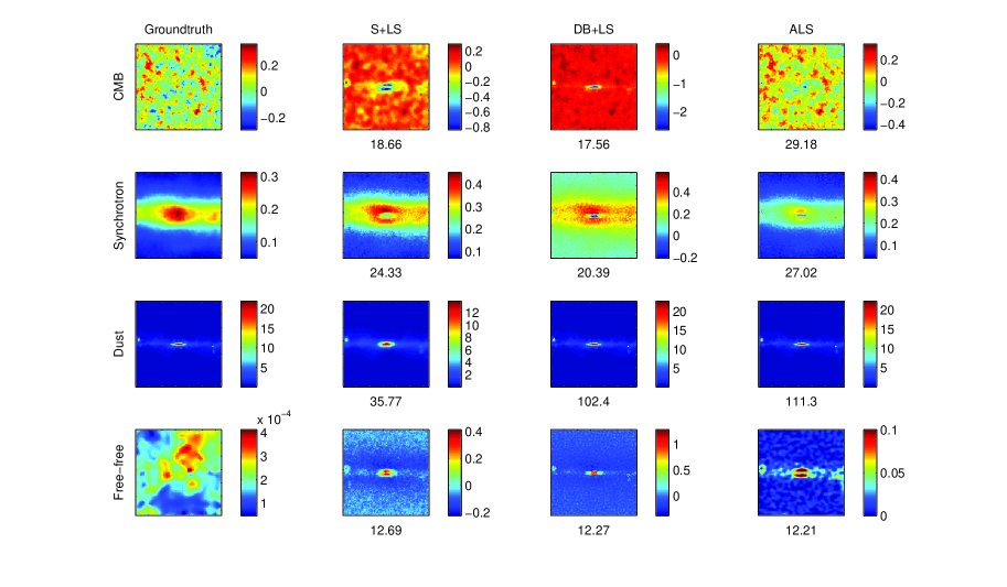
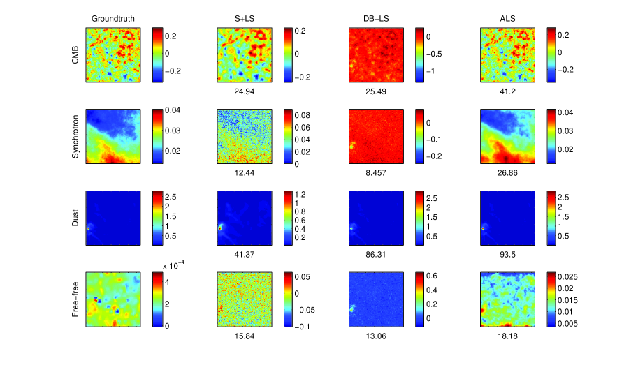
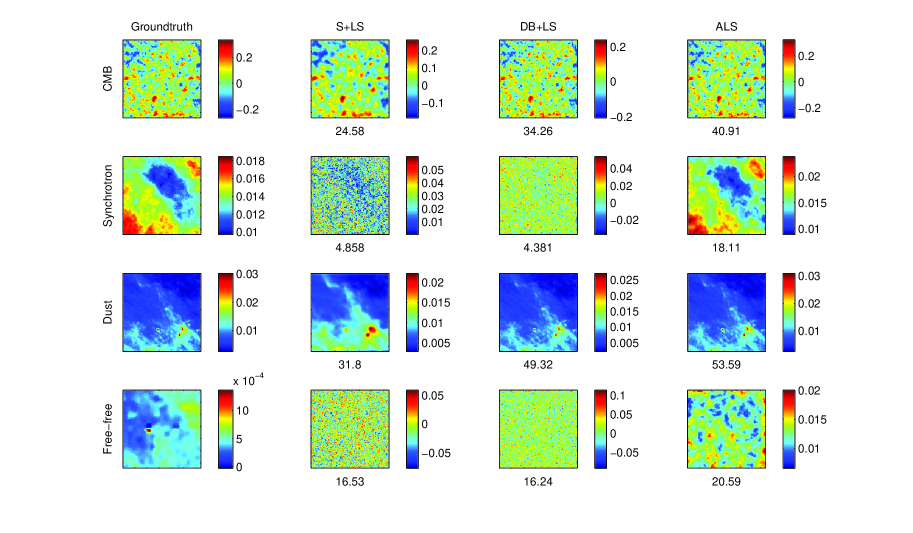
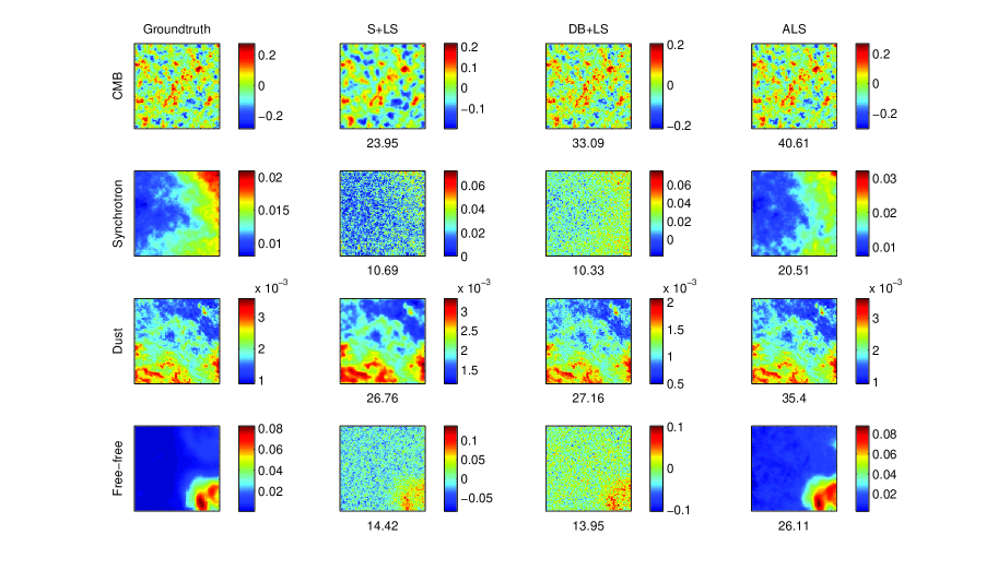
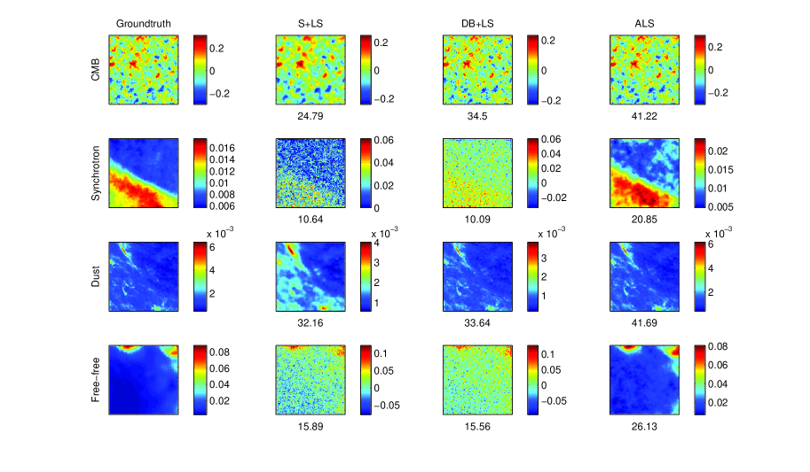
For the patch (0,0), we obtained a good reconstruction for CMB with the proposed method (Fig. 1). In the middle of the map, the effect of the dust has been already seen. The effect of the dust also exists in the synchrotron map. The free-free component radiation map in the patches (0,0), (0,20) and (0,40) cannot be estimated by any method, since its intensity is very weak. For all the patches, the proposed method reconstructs better the CMB and the foreground maps in the sense of .
We also estimate the error in the maps. Using MC samples, we can find the uncertainty in the estimation. We call this MC error and calculate its standard deviation for single pixel as
| (24) |
where the number is the ending point of the simulation. We use 100 iterations after convergence, so in this study .
We obtain another error measure by fitting a Gaussian to the posterior of the source image using the Laplace Approximation (LA) method and calculating the standard deviation, , of the approximated Gaussian. Table 2 lists the average standard deviations , and of the reconstruction, the Monte Carlo and the Laplace Approximation (LA) errors, respectively. The reconstruction error is always greater than the estimated errors. MC and LA errors are quite close to each other. The minimum errors for CMB are found in the patches (0,20) and (0,40).
| CMB | Synchrotron | Dust | Free-Free | |
|---|---|---|---|---|
| 30.49e-3 | 13.82e-3 | 15.04e-3 | 16.32e-3 | |
| 2.38e-3 | 0.42e-3 | 0.08e-3 | 1.50e-3 | |
| 3.38e-3 | 0.14e-3 | 0.06e-3 | 1.28e-3 | |
| CMB | Synchrotron | Dust | Free-Free | |
|---|---|---|---|---|
| 14.83e-3 | 2.26e-3 | 1.03e-3 | 12.80e-3 | |
| 2.81e-3 | 1.04e-3 | 0.03e-3 | 2.10e-3 | |
| 3.37e-3 | 0.92e-3 | 0.06e-3 | 1.46e-3 | |
| CMB | Synchrotron | Dust | Free-Free | |
|---|---|---|---|---|
| 14.22e-3 | 2.47e-3 | 0.17e-3 | 12.25e-3 | |
| 2.88e-3 | 1.28e-3 | 0.03e-3 | 1.96e-3 | |
| 3.37e-3 | 1.12e-3 | 0.02e-3 | 1.48e-3 | |
| CMB | Synchrotron | Dust | Free-Free | |
|---|---|---|---|---|
| 10.72e-3 | 2.85e-3 | 0.06e-3 | 8.27e-3 | |
| 2.72e-3 | 1.34e-3 | 0.02e-3 | 2.05e-3 | |
| 3.37e-3 | 1.05e-3 | 0.02e-3 | 1.53e-3 | |
| CMB | Synchrotron | Dust | Free-Free | |
|---|---|---|---|---|
| 10.29e-3 | 3.21e-3 | 0.06e-3 | 7.40e-3 | |
| 2.83e-3 | 1.43e-3 | 0.02e-3 | 2.11e-3 | |
| 3.37e-3 | 1.11e-3 | 0.02e-3 | 1.54e-3 | |
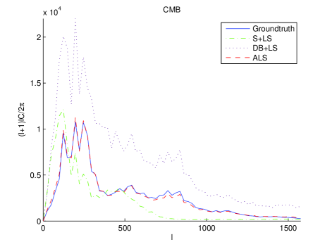
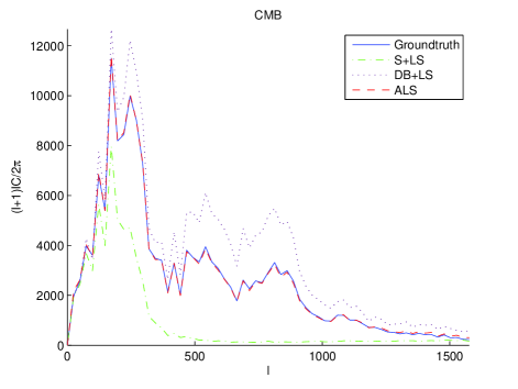
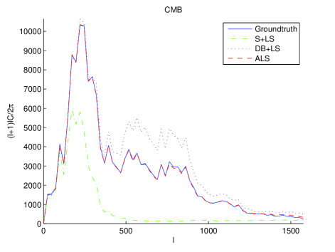
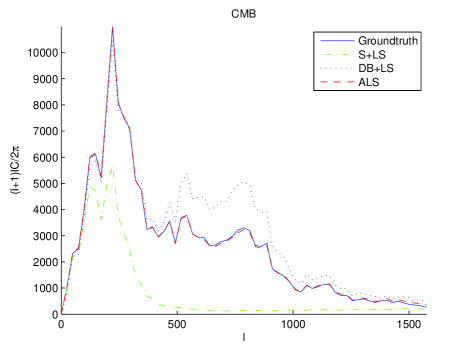
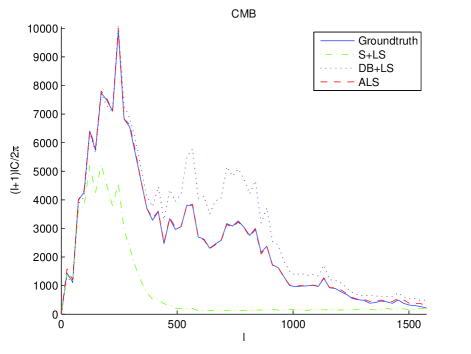
The plots in Fig. 6 compare the angular power spectrum, defined as , of the ground-truth CMB maps and those obtained by S+LS, DB+LS and the proposed ALS methods. To plot , we sample it by taking samples in the interval where . All the patches, the power spectra found by the proposed ALS method fit the ground-truth spectra more tightly than the others. The S+LS method gives bad results in the high frequency regions of the spectrums because of smoothing. The DB+LS method causes an attenuation in the low frequency regions. The root mean square error between the groundtruth angular power spectrum of CMB and those obtained by S+LS, DB+LS and proposed ALS methods are presented in Table 3. The proposed method provide one order of the magnitude better fit than the others.
| S+LS | DB+LS | ALS | |
|---|---|---|---|
| 2.1798e+3 | 7.4638e+3 | 0.1894e+3 | |
| 2.1867e+3 | 0.5742e+3 | 0.0605e+3 | |
| 2.2902e+3 | 1.5089e+3 | 0.0436e+3 | |
| 2.2261e+3 | 1.5380e+3 | 0.0462e+3 | |
| 2.1598e+3 | 1.4089e+3 | 0.0513e+3 |
6 Conclusions
We have introduced a Bayesian joint separation and estimation method for astrophysical images. The method is based on a Monte Carlo technique and gives better reconstruction in the pixel domain and frequency domain than two competitor methods. The algorithm works quite well at high latitudes. If we approach the galactic plane, the estimation results get worse. Especially at the galactic plane, we have obtained the worst results, although we have used a different initialization strategy.
Our new goal is the application of the proposed algorithm to whole-sky maps. To avoid the difficulties inherent in this problem, we plan to use the ”nested numbering” structure provided by the HEALPix (Gorski et al., 2005) package. In this format, we can reach the indexes of the eight neighbors of each pixel on the sphere. To calculate the pixel differences, we will implement a gradient calculation method on the sphere by taking the non-homogeneous spatial distances between the pixels on the sphere into consideration.
Acknowledgments
The authors would like to thank Anna Bonaldi,(INAF, Padova, Italy), Bulent Sankur, (Bogazici University, Turkey) and Luigi Bedini (ISTI, CNR, Italy) for valuable discussions. The simulated source maps are taken from the Planck Sky Model, a set of maps and tools for generating realistic Planck simulations made available thanks to the efforts of the Planck Working Group 2 (WG2) team. Some of the results in this paper have been derived using the HEALPix Gorski et al. (2005) package.
Koray Kayabol undertook this work with the support of the ”ICTP Programme for Training and Research in Italian Laboratories, Trieste, Italy, through a specific operational agreement with CNR-ISTI, Italy. Partial support has also been given by the Italian Space Agency (ASI), under project COFIS (Cosmology and Fundamental Physics). The project is partially supported by CNR-CSIC bilateral project no: 2008IT0059.
References
- Anthoine (2005) Anthoine S., 2005, PhD Thesis, Princeton University
- Becker & Le Cun (1989) Becker S., Le Cun Y., 1989, Proc. of the 1988 Connectionist Models Summer School, 29
- Bedini et al. (2005) Bedini L., Herranz D., Salerno E., Baccigalupi C., Kuruoğlu E.E., Tonazzini A., 2005, EURASIP Journal on Applied Signal Processing, 15, 2400
- Bedini & Salerno (2007) Bedini L., Salerno E., 2007, Lecture Notes in Artificial Intelligence, 4694, 9
- Belouchrani et al. (1997) Belouchrani, A., A.-Meraim, K., Cardoso, J.-F., Moulines, E., 1997, IEEE Trans. Signal Process., 45, 434
- Bonaldi et al. (2007) Bonaldi A., Ricciardi S., Leach S., Stivoli F., Baccigalupi C., De Zotti G., 2007, MNRAS, 382, 1791
- Cardoso et al. (2002) Cardoso J.-F., Snoussi H., Delabrouille J., Patanchon G., 2002, European. Conf. on Signal Processing, EUSIPCO’02, 561
- Castella & Pesquet (2004) Castella M., Pesquet J.-C., 2004, LNCS, ICA, 3195, 922
- Chantas et al. (2008) Chantas G., Galatsanos N., Likas A., Saunders M., 2008,, IEEE Trans. Image Process., 17, 1795
- Eriksen et al. (2008) Eriksen H.K., Jewel J.B., Dickinson C., Banday A.J., Gorski K.M., Lawrence C.R., 2008, ApJ, 676, 10
- Gorski et al. (2005) Gorski, K.M., Hivon, E., Banday, A.J., Wandelt, B.D., Hansen, K.M., Reinecke, F., Bartelmann, M., 2005, ApJ, 622, 759
- Hastings (1970) Hastings W.K., 1970, Biometrika, 57, 97
- Higdon (1994) Higdon D., 1994, PhD Thesis, University of Washingthon
- Hyvarinen & Oja (1997) Hyvarinen, A., Oja, E., 1997, Neural Computation, 9, 1483
- Kayabol et al. (2009) Kayabol K., Kuruoglu E.E., Sankur B., 2009, IEEE Trans. Image Process., 18, 982
- Kayabol et al. (2010) Kayabol K., Kuruoglu E.E., Sanz J.L., Sankur B., Salerno E., Herranz D., 2010, IEEE Trans. Image Process.
- Liu & Rubin (1995) Liu C., Rubin D.B., 1995, Statistica Sinica, 5, 19
- Maino et al. (2002) Maino D., Farusi A., Baccigalupi C., Perrotta F., Banday A.J., Bedini L., Burigana C., De Zotti G., Górski K.M., Salerno E., 2002, MNRAS, 334, 53
- Prudyus et al. (2001) Prudyus I., Voloshynovskiy S., Synyavskyy A., 2001, Int. Conf. on Telecomm. in Modern Satell., Cable and Broadcas. TELSIKS’01, 583
- Ricciardi et al. (2010) Ricciardi S., Bonaldi A., Natoli P., Polenta G., Baccigalupi C., Salerno E., Kayabol K., Bedini L., De Zotti G., 2010, MNRAS,
- Shwartz et al. (2008) Shwartz S., Schechner Y.Y., Zibulevsky M., 2008, Neurocomputing, 71, 2164
- Tauber et al. (2010) Tauber, J. A., Mandolesi, N., Puget, J.-L., Banos, T., Bersanelli, M., Bouchet, F. R., Butler, R. C., Charra, J., Crone, G., Dodsworth, J., and et al., 2010, A&A, 520, 1
- Tonazzini & Gerace (2005) Tonazzini A., Gerace I., 2005, European Conf. Signal Process., EUSIPCO
- Tonazzini et al. (2010) Tonazzini A., Gerace I., Martinelli F., 2010, IEEE Trans. Image Process., 19, 912
- Tzikas et al. (2009) Tzikas D., Likas A., Galatsanos N., 2009, IEEE Trans. Image Process., 18, 753
- Wilson et al. (2008) Wilson S., Kuruoglu E.E., Salerno E., 2008, IEEE Journal on Selected Areas in Signal Processing, 2, 685
Appendix A Algorithm
One cycle of Adaptive Langevin Sampler for source separation. The symbol denotes analytical update, the symbol denotes update by random sampling.
Find the initial mixing matrix with FDCCA Bedini & Salerno (2007).
Find the initial source images using the LS solution.
Initialize the parameters , and
for all source images,
for all directions,
produce from (11).
apply threshold tofor all pixels,
calculate
if then
else produce .if then ,
else
for all elements of the mixing matrix,