Adaptive Langevin Sampler for Separation of t-distribution Modelled Astrophysical Maps
Abstract
We propose to model the image differentials of astrophysical source maps by Student’s -distribution and to use them in the Bayesian source separation method as priors. We introduce an efficient Markov Chain Monte Carlo (MCMC) sampling scheme to unmix the astrophysical sources and describe the derivation details. In this scheme, we use the Langevin stochastic equation for transitions, which enables parallel drawing of random samples from the posterior, and reduces the computation time significantly (by two orders of magnitude). In addition, Student’s -distribution parameters are updated throughout the iterations. The results on astrophysical source separation are assessed with two performance criteria defined in the pixel and the frequency domains.
Index Terms:
Bayesian source separation, Multi-channel denoising, Metropolis-Hastings, Langevin stochastic equation, MCMC, Astrophysical images, Student’s -distribution.I Introduction
The Bayesian framework, which enables the inclusion of prior knowledge in problem formulation, has recently been utilized to improve the performance of Blind Source Separation (BSS) techniques. In the context of image separation, one obvious type of prior information is the spatial [1] or spatio-chromatic [2] dependence among the source pixels.
While there are three conditions that ensure separability of sources, namely, non-Gaussianity, non-whiteness and non-stationarity [3], we choose to exploit spatial correlation (i.e. spatial non-whiteness). The prior densities are constituted by modeling the image differentials in different directions as Multivariate Student’s -distributions [4]. The -distribution has some convenient properties for our model: If the degree of freedom parameter of the distribution goes to infinity, it approaches a normal density; conversely, if the degree of freedom parameter equals 1, the density becomes Cauchy. Therefore the -distribution is a flexible and tractable statistical model for data ranging from broad-tailed to normally distributed. The first examples of use of -distribution in inverse imaging problems can be found in [5] and [6]. In [6], it is shown that the -distribution approximates the distribution of the wavelet coefficients of an image more accurately. In recent papers, it has been used for image restoration [7] and deconvolution [8]. Notice that the degree of freedom parameter of the -distribution has the same role as the regularization parameter of the Markov Random Field (MRF) models. The MRF prior with Cauchy density, which was first proposed in [10] for inverse imaging, was used in [1] for source separation. The model used in [1] is an approximation to the -distribution, which is presented in Section V-A.
The -distribution has already been used in Bayesian audio source separation [9] to model the discrete cosine transform coefficients of the audio signals. It was reported that the -distribution prior had improved the sound quality over the finite mixture-of-Gaussians prior. In this study, to solve the Bayesian BSS problem for images without incurring in smoothing artifacts, we propose the -distribution for modeling the local pixel differences.
We use the joint posterior density of the complete variable set to obtain a joint estimate of all the variables. In this Bayesian approach, the BSS problem can be solved by maximizing the joint posterior density of the sources, the mixing matrix and the source prior model parameters [12], [13]. A method for solving the joint posterior modal estimation problem is the Iterated Conditional Mode (ICM) method, which maximizes the conditional densities sequentially for each variable [11]. If the mode of the conditional density cannot be found analytically, any deterministic optimization method can be used [13]. However, under any non-Gaussian hypothesis, ICM does not guarantee a unique global solution.
Another algorithm suitable for learning the Gaussian MRF is the Expectation-Maximization (EM) method. Using the Mean Field Approximation (MFA), the expectation step of the EM algorithm can be calculated analytically [14]. The MFA under Gaussian model assumption causes smoothing the edges in the image. The reason underlying these smoothing effects is that the Gaussian approximation violates the edge preserving property of the prior density, and the effect is proportional to the amount of noise. The image model with spatially varying variance parameter in variational Bayesian approximation can help overcome the smoothing problem [7], [8]. In [15], [14], deterministic optimization techniques have been used for the MRF. In [1], a Gibbs sampling stochastic optimization procedure is used. Since it is not possible to draw samples in a simple way due to the MRF priors in Gibbs distribution form, a Metropolis embedded Gibbs sampling has been adopted. In [1], it is reported that the Monte Carlo results with less image smoothing, but the cost of avoiding smoothing artifacts is a significant increase in the convergence time.
In this study, we propose a more efficient Monte Carlo Markov Chain (MCMC) sampling method in lieu of random walk Metropolis. To produce proposal samples in parallel, we resort to the Langevin stochastic equation [16], [17], [18], while the proposed samples are accepted or rejected by the Metropolis scheme. In statistical physics, the Langevin equation [16] is used to describe the Brownian motion of particles in a potential field and has been used to obtain a smart MC algorithm in [17]. Another parallel sampling algorithm is the Hamilton Monte Carlo, which is the generalized version of the Langevin sampler [18]. We conjecture that, with the samples produced in parallel by the Langevin equation, the convergence time of the algorithm will be significantly reduced.
Parameter estimation in Bayesian edge preserving inverse imaging problems with Gibbs distributions is a troublesome process because of the partition function. Although there are some methods [19, 20] that calculate the parameters using Monte Carlo techniques, their computational burdens are prohibitive. One can resort to the Pseudo Likelihood (PL) approximation to make the partition function separable, which is more convenient for parameter estimation with the Maximum Likelihood (ML) method. In [21], two Bayesian approaches have been used to estimate parameters, namely, the Maximum-a-Posteriori (MAP) and evidence approaches. An approach to estimate the regularization parameter from the PL approximation has been recently proposed [22]. The multivariate -distribution is also a PL approximation to MRF and has advantages over MRF in parameter calculations.
There are two types of parameters in edge preserving inverse imaging. The first one is the adaptive edge preserving parameter, which is also known as threshold parameter. We interpret the threshold parameter as the scale parameter of the -distribution. The other parameter is the regularization parameter, which adjusts the balance between the likelihood and the prior. The regularization parameter corresponds to the degree of freedom (dof) parameter of the -distribution. To estimate the scale and dof parameters of our -distribution, we use ML estimation via EM algorithm as in [30]. A similar approach has been used in [7] and [8].
In a comparative study among image source separation algorithms [1], we have found that the Bayesian formulation with MRF prior and Gibbs sampling outperformed the heuristic and the other Bayesian approaches. This work is based on [1], and aims to achieve a much faster MCMC implementation without compromising its good performance. With this goal in mind, we have been testing our algorithms on a current problem of modern astrophysics: the separation of radiation source maps from multichannel images of the sky at microwave frequencies. In particular, we have been applying our algorithm to the separation of the Cosmic Microwave Background (CMB) radiation from the galactic emission (synchrotron and thermal dust emissions) using realistically simulated sky maps.
The original contributions of the paper hinge on two aspects. First, we adopt the -distribution to build a prior model of the source maps. More specifically, the -distribution is used to model the differentials of the sources, as done by the first-order homogeneous MRF models. This is advantageous because the flexibility of the -distribution allows each source differential to assume a different model whether impulsive or Gaussian, simply by setting the dof parameter. The second contribution is the introduction of the Langevin sampling scheme in lieu of the random walk Gibbs sampling. As opposed to pixel-by-pixel sampling, Langevin sampling generates the samples in parallel, thus leading to much faster convergence. Furthermore, the samples are drawn in an informed way, since their generation follows the gradient descent direction on an energy surface.
Section II is a brief introduction to astrophysical sources. In Section III, the component separation problem in observational astrophysics is stated. Section IV lays out the Bayesian formulation of the problem. Section V presents the derivation steps of the adaptive Langevin sampler algorithm along with the EM parameter estimation method. The simulation results are presented in Section VI and interpreted in Section VII.
II An Introduction to Astrophysical Sources
Here, we only give a brief description of the astrophysical radiations considered, referring the interested reader to [23] for details. We are interested in the frequency range 30 to 1000 GHz where the dominant diffuse radiations are the CMB, the galactic synchrotron radiation and the thermal emission from galactic dust. Studying this radiation would help us to understand the distribution and the features of interstellar dust in our galaxy.
The most interesting astrophysical source in the microwave region of the electromagnetic spectrum is the CMB, a relic radiation originating from the time when the Universe was 300.000 years old. The discovery of the CMB is one of the fundamental milestones of modern cosmology and its study allows us to determine fundamental parameters such as the age of the universe, its matter and energy composition, its geometry and many other relevant cosmological parameters. CMB should be a blackbody radiation at a temperature of K, thus its emission spectrum should be perfectly known. The CMB emission dominates over the other sources at frequencies around 100 GHz. The CMB temperature is not perfectly anisotropic. Standard cosmological models predict that the CMB anisotropy is Gaussian distributed, although some alternative models permit a certain degree of non-Gaussianity. Current observations are compatible with the hypothesis of Gaussianity. Two all-sky surveys have been made on CMB so far, by NASA’s satellites COBE [32] and WMAP [33]. A European mission whose data will be highly accurate and spatially resolved, Planck [23], is about to provide its first full-sky coverage maps.
The CMB signal is mixed with other astrophysical sources of electromagnetic radiation. Relativistic electrons being accelerated by magnetic fields in the Galaxy give rise to synchrotron emission, which dominates over the CMB in regions close to the Galactic plane especially at low frequencies ( GHz). According to observations in other frequency bands, the synchrotron emission spectrum follows a power law with a negative exponent, whose value is presently known with high uncertainty. Synchrotron is the dominant radiation in the low-frequency bands of our range of interest. Inter-stellar dust grains are heated by nearby stars and re-emit thermal radiation in the far infrared region of the electromagnetic spectrum. Dust radiation is dominant in the high end of our range. In particular, it is almost the only significant contribution to the total diffuse radiation between 800 GHz and 1000 GHz. Its emission spectrum should follow a greybody law, with unknown spectral index and an additional degree of freedom given by the thermodynamical temperature of the dust grains. For a short review on CMB astronomy, see [24].
There are other astrophysical sources present at microwave frequencies, such as free-free emission due to free electrons, anomalous dust emission and radiation coming from extragalactic sources, but their relevance is smaller. In this work we will focus on the main three astrophysical sources present in CMB experiments: CMB, synchrotron and dust.
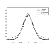
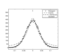
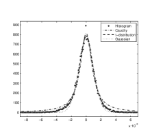
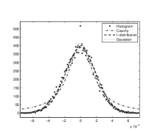
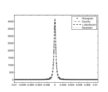
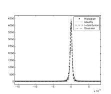
In order to justify our adoption of the Student’s -distribution in a relevant case, we have selected a sky patch, located at galactic longitude and galactic latitude, discretized into a -pixel map. Within this patch, we have introduced simulated CMB, synchrotron, and dust radiation maps (as in [26]). We have computed the source image differentials for horizontal and vertical directions, and estimated their empirical distributions. We have fitted three different functions to the empirical distributions of the image differentials of the astrophysical sources with nonlinear least square method using the Curve Fitting Toolbox of MATLAB. These functions are proportional to Gaussian, Cauchy and -distribution. Fig. 1 shows the fitting results for CMB, synchrotron and dust images. Table I lists the residual Root Mean Square Errors (RMSE) of the fits. The Gaussian gives the best fit for CMB because the CMB is theoretically distributed as a Gaussian [24]. Overall, the -distribution appears to be a good choice for modeling the image differential statistics in horizontal and vertical directions of all the components. The estimated dof parameters of -distributions show that indeed the proposed model assumes from impulsive to Gaussian characteristic underlying each component. If the component is Gaussian as CMB, the dof parameter becomes bigger and if it is impulsive, the dof parameter becomes very small.
| Horizontal direction | ||||
|---|---|---|---|---|
| Gaussian | Cauchy | -distribution | dof | |
| CMB | 15.11 | 30.84 | 15.47 | 25.71 |
| Synchrotron | 23.70 | 30.06 | 15.70 | 3.59 |
| Dust | 67.99 | 33.21 | 13.84 | 1.81 |
| Vertical direction | ||||
|---|---|---|---|---|
| Gaussian | Cauchy | -distribution | dof | |
| CMB | 15.75 | 29.70 | 15.83 | 15.75 |
| Synchrotron | 19.11 | 31.00 | 18.39 | 19.11 |
| Dust | 63.73 | 68.19 | 54.42 | 2.18 |
III Component Separation Problem in Observational Astrophysics
Virtually any application in observational astrophysics has to do with problems of component separation. Indeed, all the astrophysical observations result from the superposition of the radiation sources placed along the line of sight. While very distant sources can be distinguished by the redshift analysis, for nearby sources this is not possible. In fact, physically distinct sources can sometimes be found within a close range of each other. Furthermore, high sensitivity and high resolution measurements can give rise to source mixing problems even in the cases where the radiation under study is dominant over interfering radiations. Apart from redshift analysis, useful methods to distinguish between superimposed physically different radiations include spectral analysis and morphological analysis. In this paper, we only treat the former approach, exploiting the differences in the emission spectra shown by physically distinct radiation sources. This implies that the separation must be done on the basis of measurements made at different frequency bands.
We assume that the observed images, , are linear combinations of source images. Let the th observed image be denoted by , where represents the lexicographically ordered pixel index. The image separation problem consists in finding independent sources from different observations. If and denote vector representations of source and observation images, respectively, then the observation model can be written as
| (1) |
where is an iid zero-mean noise vector with covariance matrix and is an identity matrix. Although the noise is not necessarily homogeneous in the astrophysical maps, in this study we assume that the noise variance is homogeneous within each sky patch and is also known.
Since the observation noise is assumed to be independent and identically distributed zero-mean Gaussian at each pixel, the likelihood is expressed as
| (2) | |||||
| (3) |
where the mixing matrix contains all the mixing coefficients introduced in (1).
For many purposes, a mixing model of the type (1) is considered to fit reasonably well to an astrophysical observation. The details on how to get an equation similar to (1) from the physics of the problem can be found in [25]. Here, we only summarize the main assumptions made with this purpose. First, we assume that the superposition of the signals originating from different sources is linear and instantaneous. In the astrophysical case, this assumption is clear, since the physical quantities to be measured are superpositions of electromagnetic waves coming, for any bearing, exactly from the same line of sight without any scattering or diffraction effect. The second assumption in modeling astrophysical observations is that each source has an emission spectrum that does not vary with the bearing. This assumption implies that individual radiations result from the product of a fixed spatial template and an isotropic emission spectrum. Both assumptions need closer attention. The precise emission spectrum generated by any physical phenomenon depends on many quantities that may not all be distributed uniformly in the sky. Although in many applications the isotropy assumption has been adopted successfully, in many other cases the space-variability of the radiation sources must be taken into account to allow a good separation to be performed. Furthermore, if the effect of the telescope is taken into account, then the instantaneous model is no more valid since, for the finite aperture, the light captured in a fixed direction in the telescope does not come from that direction alone. In formulas, model (1) becomes
| (4) |
where the asterisk means convolution, and is the telescope radiation pattern in the ’th observation channel. Note that, if is the same for all the channels, (4) can be written as
| (5) |
and the problem is again instantaneous for the modified sources , which are the physical sources smoothed by the common radiation pattern . Unfortunately, especially in the radio- to millimeter-wave ranges, the telescope aperture depends strongly on frequency, and model (5) cannot be adopted directly, unless the observed signals are preprocessed to reduce their angular resolution to the worst available (see [26]).
Since no imaging system can achieve an infinite resolution, we should use (4) as our generative model. However, to avoid problems with the convolutive mixtures, we assume to have a telescope with the same radiation pattern in all the channels, so as to be able to use model (5). Note that this can always be obtained by preprocessing, provided that all the beam patterns are known. Hereafter, as it will not cause any ambiguity, we drop the tilde accent from the symbols used to denote the data and the source vectors.
IV Source Separation Defined in the Bayesian Framework
IV-A Source Model
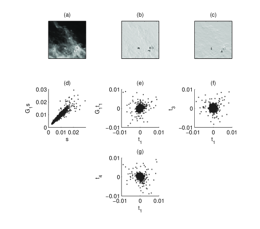
Neighbor pixels in our images have strong dependency. This is demonstrated, for example, in Fig. 2(d) where the scatter-plot shows the first order right neighbor pixels of the dust map shown in Fig. 2(a). The dependency decreases in the high intensity region. This region in the scatter-plot corresponds to spatially localized structures with high image intensity of the map in Fig. 2(a). The existence of a small number of point-like structures in the maps indicates that the dependency assumption is valid. In view of this, we can write an auto-regressive source model using the first order neighbors of the pixel:
| (6) |
where denotes one of the main directions (left, right, up and down) and is the cardinality of the set of image differential directions. Matrix is a linear one-pixel shift operator in direction , is the regression coefficient and the regression error is an iid -distributed zero-mean vector with dof parameter and scale parameters , . We can justify the iid assumption of by plotting (see Fig. 2(e)) the values in versus its first order neighbors, . We can interpret as a decorrelated version of . Fig. 2(b) shows for . By comparing Fig. 2(d) and (e), we can say that is spatially more independent than .
If the image were Gaussian distributed, then the regression error would also be Gaussian. However in real images, the regression error is better modelled by some heavy-tailed distribution. The -distribution can conveniently model the statistics of data whose distribution ranges from Cauchy to Gaussian, and therefore it is a convenient model for the statistics of the high spatial frequency contents of images, such as regression errors [6]. The scale parameter can be assumed as a space-varying parameter to model the highly non-stationary sources, i.e. sparse sources, but homogenous variance assumption has been observed to be adequate for diffuse astrophysical source images for the image patch sizes that we use in the simulations. We use a homogeneous variance since, in our case, the increased complexity derived from inhomogeneity is not justified by a significant improvement in performance.
The regression error represents the directional image differential in the direction . The multivariate probability density function of an image modelled by a -distribution can be defined as
| (7) | |||||
where and is the Gamma function. We can write the density of by using the image differentials in different directions, assuming directional independence, as where . We can simply justify this assumption by plotting the horizontal regression error versus the vertical one as shown in Fig. 2(f). We can observe in this figure that the scatter plot of the regression errors in left and up directions is almost circular and this justifies our assumption of independence. Fig. 2(g) shows the scatter-plot of right difference versus left difference. In spite of a weak dependence between right and left difference images, we maintain the independency assumption to constitute the products of the regression error probabilities model. A similar approach to constitute a single prior by multiplying different individual priors can be found in [27]. In this study, we use the left/right and up/down differences jointly in the prior model to balance their contributions. Otherwise, we could obtain directionally biased results.
The -distribution can be written in implicit form by using a Gaussian and a Gamma density. The -distribution has a dof parameter , which is itself governed by Gamma distribution with parameter . The -distribution has the following form [30]:
| (8) |
The interpretation of this equation is that if is distributed with a normal density and the parameter has a Gamma prior as , the distribution of becomes a -distribution such that . The representation in (IV-A) is a particular case of the Gaussian Scale Mixture (GSM) densities. The ML estimation of the parameters , and using the EM method [30] is given in Section V-B.
IV-B Posteriors
The joint posterior density of all the unknowns in the BSS problem can be written as:
| (9) |
where is the likelihood and is the joint prior density of unknowns. The joint prior can be factorized as . Furthermore, since the sources are assumed to be independent, the joint probability density of the sources is also factorized as .
Mathematically, we can assume uniform priors for , and , because ’s are always positive. The practical usage of these priors is explained in Section V-D. We use a conjugate Gamma prior for . We have determined the respective parameters experimentally. The conditional posteriors of all model parameters are written as
| (10) | |||||
where expressions in the subscripts denote the removal of that variable from the variable set. The parameters , and have size , has size and the sources have size . Overall there are unknowns.
For parameters , and , we exploit the EM method. To estimate the source images, we use a version of the posterior augmented by auxiliary variables and find the estimation with a Langevin sampler. The details are given in Section V.
V Estimation of Sources and Parameters
In this section, we give the details of the estimation of the sources and the parameters.
V-A Sources
We modify the posterior densities of the source images to obtain a more efficient MCMC sampler. In the classical MCMC schemes, a random walk process is used to produce the proposal samples. Although random walk is simple, it affects adversely the convergence time. The random walk process only uses the previous sample for producing a new proposal. Instead of a random walk, we use the Langevin stochastic equation, which exploits the gradient information of the energy function to produce a new proposal. Since the gradient directs the proposed samples towards the mode, the final sample set comes mostly from around the mode of the posterior [28], [29].
The Langevin equation can be obtained from the total energy function. We first define everything in continuous time to give the derivation steps of the Langevin equation, then we transfer them into discrete time. To obtain the total energy function, we introduce a velocity parameter to define the kinetic energy such that
| (11) |
where is a diagonal matrix whose diagonal elements correspond to mass parameters for pixel index . Using the velocity parameter , the modified version of the posterior density in (IV-B) is written as . More explicitly, it can be written as
| (12) |
where the energy function of a source image can be written in terms of image differentials as
| (13) |
where the function is proportional to the negative logarithm of the -distribution in (7), that is,
| (14) |
and the function is the regularization function proposed in [10]. The terms and correspond to the regularization and the threshold parameters, respectively, used in edge preserving image reconstruction.
The energy function was defined in (3). The total energy function is proportional to the negative logarithm of the posterior. In summary, the three terms correspond, respectively, to the fit to data and to the inertial and the kinetic energy terms. We can define the Lagrangian function: and write the Lagrange-Euler equation for the Lagrangian as follows
| (15) |
| (16) |
where . If we discretize the dynamics in (16) and velocity using the Leapfrog method [18], we obtain the following three-step iteration
| (17) | |||||
| (18) | |||||
| (19) |
where , is the gradient with respect to and is the discrete time step. If we define a diagonal matrix , so that, for the th pixel, the diffusion coefficient is . Matrix is referred to here as the diffusion matrix, and is derived in Section V-A1. Instead of this step scheme, we use the one-step Langevin difference equation. To obtain the single step Langevin update equation for , we substitute (17) into (18).
| (20) |
This form is also used in [28], [29]. The samples are produced by using this first order equation, and then they are tested in the Metropolis-Hastings scheme.
If we assume the transitions in (20) as a Wiener process and take into account the fact that the velocity vector is independent of the source vector , [18], then its probability density function can be set as a multivariate Gaussian as . We can produce a random sample from this probability such that where is a zero-mean Gaussian vector with identity covariance matrix . If we substitute this random sample into (20), we obtain the associated Langevin equation
| (21) |
Since the random variables for the image pixel intensities are produced in parallel by using (21), the procedure is faster than the random walk process adopted in [1]. The random walk process produces local random increments independently from the neighbor pixels and the observations. In the Langevin sampler, the samples are generated in an interrelated manner and in terms of the descent of an energy function that reflects the goodness of the model fit. Once the candidate sample image is produced by (21), the accept-reject rule is applied independently to each pixel. In the case of random walk, we would produce the candidate sample pixel and apply the accept-reject rule. The sampling of the whole image would be completed by scanning all the pixels in a sequential order as in Gibbs sampling. Since each pixel has to wait the update of the previous pixel, this procedure is very slow. In random walk, candidate pixels can be produced in parallel but, producing a candidate sample for the whole image using random walk is not a reasonable method because hitting the right combination for such a huge amount of data (i.e. ) is almost impossible. By Langevin sampler, the likelihood of approximately hitting the right combination at any one step is much higher.
After their production, the samples are tested via Metropolis-Hastings [34] scheme pixel-by-pixel. The acceptance probability of any proposed sample is defined as , where
| (22) |
where and . For any single pixel, can be derived from (13) and (14) as
| (23) |
The proposal density is obtained, from (21), as
| (24) |
One cycle of the Metropolis-Hastings algorithm embedded in the main algorithm, for each source image, is given in Table II.
-
1.
-
2.
-
3.
-
4.
-
5.
produce from (21).
-
6.
for all pixel
-
(a)
calculate
-
(b)
if then
else produce .if then ,
else -
(c)
next pixel.
-
(a)
V-A1 Diffusion Matrix
In this section, we give a method to find an optimum diffusion matrix . The method must ensure that the produced sample comes from the joint conditional distribution introduced in (V-A). If we write the Taylor expansion of with the infinitesimal and take the expectation of both sides with respect to the joint density , we obtain the following equation
where is the Hessian matrix of with respect to . From this equation, the optimum infinitesimal is found as .
If we also take the expectation of both sides of (20), we obtain
| (25) |
and comparing with (25), we write . Rather than the expectation of the inverse of Hessian matrix, we use its diagonal calculated by the value of at the discrete time as
| (26) |
where and operator extract the main diagonal of the Hessian matrix. From (26), we can find the diffusion parameter as [35]:
| (27) |
This approximation is justified if is strongly diagonally dominant.
V-B Parameters of -distribution
We can write the joint posterior of the parameters , and such that . Using the likelihood in (IV-A) and the priors of the parameters, we can find the MAP estimates of the parameters of the -distribution by EM method. Instead of maximizing the , we maximize the following function
| (28) | |||
where is the posterior density of the hidden variable conditioned on parameters estimated in the previous step and represents the expectation with respect to . For simplicity, hereafter we use only to represent this expectation. The parameter is a hidden (or latent) variable that changes the scale of the Gaussian density and has a Gamma prior . By exploiting , we can define the -distribution as a scale mixture of Gaussians as in (IV-A). The second term on the righthand side of (28), , corresponds to the entropy of the posterior density of , and is independent of the unknowns, and the function
| (29) |
The aim is to find the maximum of with respect to ;
| (30) |
In the E (expectation) step of the EM algorithm, we must calculate the expectation . For this purpose, we find the posterior density of
| (31) |
The expectation of is
| (32) |
In the M (maximization) step, (29) is maximized with respect to . To maximize this function, we alternate among the variables , and . After taking the logarithms and expectations in (29), the cost functions for , and are written as follows
| (33) |
| (34) |
| (35) |
The maximization of (35) does not have a simple solution. It can be solved by setting its first derivative to zero:
| (38) |
where is the first derivative of and it is called digamma function.
V-C Parameters of the Mixing Matrix
We assume that the prior of is uniform between 0 and . The conditional density of is expressed as . From (2), it can be seen that the conditional density of becomes Gaussian. The parameter is estimated in each iteration as
| (39) |
where is the unit step function.
V-D Adaptive Langevin Sampler Algorithm
The proposed Adaptive Langevin Sampler algorithm is given in Table III. The symbol denotes analytical update, the symbol denotes update by finding the zero root and the symbol denotes the update by random sampling. The sampling of the sources is done by the Metropolis-Hastings scheme given in Table II. To deal practically with uniformly distributed positive variables, we assume that they lie in the range .
V-D1 Initialization
We start the algorithm with the mixing matrix obtained by the FDCCA (Fourier Domain Correlated Component Analysis) [31] method. The initial values of astrophysical maps are obtained by Least Square (LS) solution with the initial mixing matrix. The initial values of can be calculated directly from image differentials. We initialized the and found the initial value of by equaling the expectation (32) to a constant. In this study, we take the initial value of this posterior expectation . So the initial value of
V-D2 Stopping Criterion
We observe the normalized absolute difference between sequential values of to decide the convergence of the Markov Chain to an equilibrium. If , we assume the chain has converged to the equilibrium for and denote this point . Since we have parallel chains for sources, the ending point of the burn-in period of the whole Monte Carlo chain is . We ignore the samples before . We keep the iteration going until that is the ending point of the post burn-in period simulation. In the experiments, we have used 100 iterations after burn-in period, so .
VI Simulation Results
To test our procedure, we assume nine observation channels with center frequencies in the range 30–857 GHz, where the dominant diffuse radiations are the CMB, the galactic synchrotron radiation and the thermal emission from galactic dust. Except for CMB, these radiations have unknown emission spectra (that is, the coefficients in (1) are not all known). Both observation models in (1) and (5) are suitable for our algorithm. In the experiments, we assume the model in (1), that is of instantaneous mixtures and isotropic sky, to be valid. We plan to attack the problems of space variability and channel-dependent convolutional effects in the future.
In the sequel, we present astrophysical image separation results on a comparative basis. The proposed method is denoted as ALS-t (Adaptive Langevin Sampler--distribution) and is compared to four other methods, namely: 1) GS-MRF, which is the MRF model coupled with Gibbs sampling [1]; 2) LS, which forms our initial estimates on the basis of the values of obtained by FDCCA [31]; 3) Iterated Conditional Modes (ICM), which maximizes the conditional pdfs sequentially for each variable [11]; 4) ALM-MRF, which is the solution of the MRF model via Langevin and Metropolis-Hastings schemes [22].
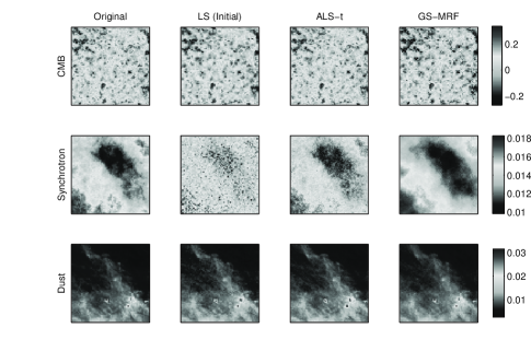
The leftmost column of Fig. 3 shows the ground-truth simulated astrophysical source maps. The remaining columns show the source maps separated by LS, ALS-t and GS-MRF, respectively. The sky patch used for this experiment is centered at longitude and latitude in galactic coordinates and has a size of square degrees in the celestial sphere, discretized in a pixel map.
The Peak Signal-to-Interference Ratio (PSIR) is used as a numerical performance indicator. The PSIR can be calculated if the ground-truth is known, which is the case in our work since all sky components are simulated. For this patch, the algorithm converges after 155 iterations and uses a total of 255 iterations to reach the solution (see Fig. 4). We compare the results with the ones of LS, ICM, GS-MRF and ALM-MRF.
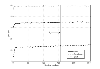
Table IV lists the PSIR values and the process times. The simulations are run on a Core2 CPU 1.86 GHz PC. The process time of ALS-t is much shorter than that of the GS-MRF. The execution time of ALS-t is two orders of magnitude smaller than that of GS-MRF. The PSIR values of ALS-t are also over those of LS, ALM-MRF, GS-MRF and ICM, especially for synchrotron, and furthermore, the smoothing degradation of ICM on the synchrotron component is not observed in the proposed method , Fig. 3.
| CMB | Synchrotron | Dust | time | |
|---|---|---|---|---|
| LS | 30.69 | 15.03 | 37.37 | 1.32e-4 |
| ICM | 26.27 | 17.64 | 35.30 | 0.31 |
| GS-MRF, [1] | 27.81 | 22.33 | 38.93 | 226.72 |
| ALM-MRF, [22] | 27.91 | 20.88 | 36.41 | 2.86 |
| ALS-t | 33.45 | 26.21 | 40.51 | 1.65 |
| CMB | Synchrotron | Dust | |
|---|---|---|---|
| 3.01 | 10.01 | 4.08 | |
| 1.80 | 4.54 | 1.78 |
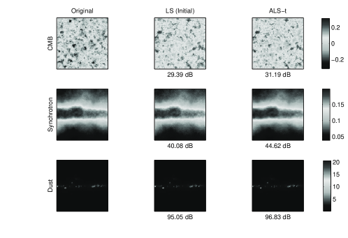
We have also run the algorithm for pixels patches centered at and . Fig. 5 shows the results for the patch . In that patch, the relative intensity of CMB is the weakest one. The PSIR values of the estimates of LS and ALS-t are written under the maps and the PSIR improvements are listed for that patch and for the patch in Table V. The total time of the ALS-t algorithm for the size patches is about minutes.
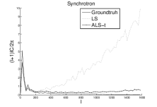
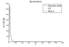
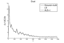
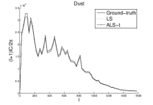
We also use an alternative performance criterion, defined in the spherical harmonic (frequency), , domain, since the angular power spectrum is relevant to astrophysics. If we decompose a CMB map on spherical harmonics, the complex coefficients, (, ), define the angular power spectrum, , as the average .
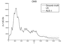
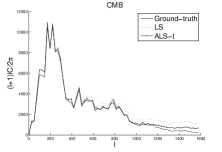
In Fig. 6, we plot the standard power spectrum, , defined as of the original and the reconstructed sources in the two patches considered. In order to compare different methods, we also introduce the Peak Signal-to-Interference Ratio in the -domain defined as
| (40) |
where is the estimated power spectrum.
In the off-galactic patch considered in Fig. 6, the intensity of synchrotron is very low and the LS solution for synchrotron is contaminated too much by noise. The estimated CMB and the dust spectrums by ALS-t follow the ground-truth spectrum better than the LS one, especially in the high frequency regions. For the patch , synchrotron and dust are estimated adequately by LS, but the LS estimate of CMB is improved by ALS-t. The related PSIRspec values are presented in Table VI.
| , | , | |||||
|---|---|---|---|---|---|---|
| CMB | Synch. | Dust | CMB | Synch. | Dust | |
| LS | 30.33 | 2.65 | 37.76 | 31.59 | 45.69 | 39.35 |
| ALS-t | 35.87 | 26.23 | 40.69 | 34.53 | 46.98 | 38.93 |
We have observed that the estimated regression parameter is quite isotropic for all the maps. For the CMB map in the patch, its value is about for all . In the same patch, the values of the parameter for synchrotron and dust are . These results show us that the CMB radiation is spatially less correlated than the other radiation sources. We assume the parameter is isotropic and estimate a single value for each direction. The EM estimation of depends too much on its prior and initial value. We have allowed the parameter to be anisotropic, but at the end of the estimation steps we have found that it is almost isotropic for all radiation maps.
VII Conclusion and Future Work
We have developed a Bayesian source separation algorithm for astrophysical images where the MCMC samples are generated through the Langevin stochastic equation. The proposed algorithm provides two orders of magnitude computational economy vis-à-vis the Gibbs sampling approach. In addition, it generates better source separation as compared to all its competitors, i.e., LS, ICM, ALM-MRF and GS-MRF methods measured in terms of PSIR in the pixel domain and PSIRspec in the annular frequency domain. The algorithm can reconstruct the high frequency regions of the power spectrums with higher fidelity. A byproduct of this approach is the capability to estimate the parameters of the -distribution image priors. Although the proposed ALS-t method takes longer than either ICM or LS methods, its superior performance by far outweighs this disadvantage, and furthermore the algorithm lends itself to parallel processing. To improve the algorithm performance, non-stationary image priors, more efficient discretization time step and diffusion matrix can be investigated in the future. Another point to obtain a beneficial algorithm might be the usage of more than one MH-steps, because the EM algorithm which estimates parameters converges faster than the Monte Carlo sampling scheme.
Our new goal is the application of the proposed algorithm to whole-sky maps. To avoid the difficulties inherent in this problem, we plan to use the ”nested numbering” structure provided by the HEALPix [37] package. In this format, we can reach the indexes of the eight neighbors of each pixel on the sphere. To calculate the pixel differences, we will implement a gradient calculation method on the sphere by taking the non-homogeneous spatial distances between the pixels on the sphere into consideration.
Other issues to be addressed are the channel-dependent blurring effects of the antennas and the non-stationary nature of noise. We have to reformulate the source separation problem without these simplifying assumptions on the observations. Finally, a pixel-based estimation error is being analyzed with the goal of defining a stopping criterion for the algorithm.
Acknowledgment
References
- [1] K. Kayabol, E. E. Kuruoglu and B. Sankur, “Bayesian separation of images modelled with MRFs using MCMC,” IEEE Trans. Image Process., vol.18, no.5, pp. 982–994, May 2009.
- [2] K. Kayabol, and E. E. Kuruoglu, and B. Sankur, “Image Source Separation using Color Channel Dependencies,” in ICA 2009, LNCS, vol. 5441, pp. 499–506, Paraty, Brasil, Springer-Verlag, 2009.
- [3] J.-F. Cardoso, “The three easy routes to independent component analysis; Contrasts and Geometry,” in Int. Conf. on Indepen. Comp. Anal. ICA’01, San Diego, Dec. 2001.
- [4] Student (W. S. Gosset), “The probable error of a mean,” Biometrika, vol.6, no.1, pp. 1–25, 1908.
- [5] D. Higdon, Spatial Applications of Markov Chain Monte Carlo for Bayesian Inference. PhD Thesis, University of Washingthon, 1994.
- [6] I. Prudyus, S. Voloshynovskiy and A. Synyavskyy, “Wavelet-based MAP image denoising using provably better class of stochastic i.i.d. images models,” in Int. Conf. on Telecomm. in Modern Satell., Cable and Broadcas. TELSIKS’01, pp. 583–586, Sep. 2001.
- [7] G. Chantas, N. Galatsanos, A. Likas and M. Saunders, “Variational Bayesian image restoration based on a product of t-distributions image priors,” IEEE Trans. Image Process., vol.17, no.10, pp. 1795–1805, Oct. 2008.
- [8] D. Tzikas, A. Likas and N. Galatsanos, “Variational Bayesian sparse kernel-based blind image deconvolution with Student’s-t priors,” IEEE Trans. Image Process., vol.18, no.4, pp. 753–764, Apr. 2009.
- [9] C. Fevotte and S. J. Godsill “A Bayesian approach for blind separation of sparse sources,” IEEE Trans. Audio, Speech Language Process., vol. 14, no. 6, pp. 2174–2188, Nov. 2006.
- [10] T. Hebert and R. Leahy, “A generalized EM algorithm for 3-D Bayesian reconstruction from Poisson data using Gibbs priors,” IEEE Trans. Medical Imaging, vol.8, no.2, pp. 194–202, June 1989.
- [11] D. B. Rowe, “A Bayesian approach to blind source separation,” Journal of Interdisciplinary Mathematics, vol.5, no.1, 2002.
- [12] K. H. Knuth, “A Bayesian approach to source separation, ” in Int. Conf. on Indepen. Comp. Anal. ICA’99, pp. 283–288, Jan. 1999.
- [13] A. Mohammad-Djafari, “A Bayesian approach to source separation,” in Int. Workshop on Maximum Entropy and Bayesian Methods, MaxEnt’99, July, 1999.
- [14] A. Tonazzini, L. Bedini, and E. Salerno “A Markov model for blind image separation by a mean-field EM algorithm,” IEEE Trans. Image Process., vol. 15, pp. 473–482, Feb. 2006.
- [15] E. E. Kuruoglu, A. Tonazzini, and L. Bianchi, “Source separation in noisy astrophysical images modelled by Markov random fields,” in Int. Conf. on Image Proc. ICIP’04, pp. 24–27, Oct., 2004.
- [16] P. Langevin, “Sur la theorie du mouvement brownien,” (On the theory of Brownian motion), C.R. Acad. Sci., (Paris), vol. 146, pp. 530 -533, 1908.
- [17] R.J. Rossky, J.D. Doll, and H.L. Friedman, “Brownian dynamics as a smart Monte Carlo simulation,” J. Chem. Phys., vol. 69, pp. 4628–4633, 1978.
- [18] R.M. Neal, “Probabilistic inference using Markov chain Monte Carlo methods,” Tech. Rep. CRG-TR-93-1, Dept. Comp. Scien., University of Toronto”, Sep. 1993.
- [19] D.M. Higdon, J.E. Bowsher, V.E. Johnson, T.G. Turkington, D.R. Gilland, and R. J. Jaszczak”, “Fully Bayesian estimation of Gibbs hyperparameters for emission computed tomography data,” IEEE Trans. Medical Imaging, vol. 16, no. 5, pp. 516–516, Oct. 1997.
- [20] X. Descombes, R.D. Morris, J. Zerubia, and M. Berthod, “Estimation of Markov random field prior parameters using Markov chain Monte Carlo maximum likelihood,” IEEE Trans. Image Process.”, vol. 8, no. 7, pp. 954–963, July 1999.
- [21] R. Molina, A. K. Katsaggelos and J. Mateos, “Bayesian and regularization methods for hyperparameter estimation in image restoration,” IEEE Trans. Image Process.”, vol. 8, no. 2, pp. 231–246, Feb. 1999.
- [22] K. Kayabol, E. E. Kuruoglu, B. Sankur, E. Salerno and L. Bedini, “Fast MCMC separation for MRF Modelled astrophysical components,” in Int. Conf. on Image Proc. ICIP’09, pp. 2769–2772, Nov. 2009.
- [23] Planck Science Team, “PLANCK: The scientific programme,” European Space Agency (ESA), 2005. [Online]. Available: http://www.esa.int/SPECIALS/Planck/index.html
- [24] W. Hu and S. Dodelson, Cosmic Microwave Background Anisotropies, Annual Review of Astronomy and Astrophysics, vol. 40, pp. 171 -216, 2002.
- [25] C. Baccigalupi, L. Bedini, C. Burigana, G. De Zotti, A. Farusi, D. Maino, M. Maris, F. Perrotta, E. Salerno, L. Toffolatti, A. Tonazzini “Neural networks and the separation of cosmic microwave background and astrophysical signals in sky maps,” Mon. Not. Royal Astronom. Soc., vol.318, pp. 769-780, 2000.
- [26] C. A. Bonaldi, L. Bedini, E. Salerno, C. Baccigalupi, and G. De Zotti, “Estimating the spectral indices of correlated astrophysical foregrounds by a second-order statistical approach,” Mon. Not. Royal Astronom. Soc., vol.373, 271-279, 2006.
- [27] G. E. Hinton,“Products of experts,” in Int. Conf. on Artificial Neural Net. ICANN’99, vol. 1, pp. 1–6, 1999.
- [28] U. Grenander and M. I. Miller, “Representations of knowledge in complex systems (with discussion), ” J. R. Statist. Soc. B”, vol. 56, pp. 549–603, 1994.
- [29] P. Dostert, Y. Efendiev, T. Y. Hou and W. Luo, “Coarse-gradient Langevin algorithms for dynamic data integration and uncertainty quantification, ” J. Comput. Phys.”, vol. 217, pp. 123–142, 2006.
- [30] C. Liu and D. B. Rubin, “ML estimation of the t distribution using EM and its extensions, ECM and ECME,” Statistica Sinica”, vol. 5, pp. 19–39, 1995.
- [31] L. Bedini, and E. Salerno, “Extracting astrophysical source from channel-dependent convolutional mixtures by correlated component analysis in the frequency domain,” in Lecture Notes in Artificial Intelligence, vol. 4694, pp. 9–16, Springer-Verlag, 2007.
- [32] National Aeronautics and Space Administration, “Cosmic Background Explorer,” NASA. [Online]. Available: http://lambda.gsfc.nasa.gov/product/cobe/
- [33] National Aeronautics and Space Administration, “Wilkinson Microwave Anisotropy Probe,” NASA. [Online]. Available: http://map.gsfc.nasa.gov/
- [34] W. K. Hastings, “Monte Carlo sampling methods using Markov chains and their applications,” Biometrika”, vol. 57, no. 1, pp. 97–109, Apr. 1970.
- [35] S. Becker and Y. Le Cun, “Improving the convergence of back-propagation learning with second-order methods,” in Proc. of the 1988 Connectionist Models Summer School, pp. 29–37, 1989.
- [36] L. Bedini, D. Herranz, E. Salerno, C. Baccigalupi, E. Kuruoglu, A. Tonazzini, ”Separation of correlated astrophysical sources using multiple-lag data covariance matrices”, Eurasip J. on Appl. Sig. Proc., vol. 2005, no. 15, pp. 2400-2412, Aug. 2005.
- [37] K. M. Górski, E. Hivon, A. J. Banday, B. D. Wandelt, F. K. Hansen, M. Reinecke, M. Bartelmann, ”HEALPix: A framework for high-resolution discretization and fast analysis of data distributed on the sphere”, The Astrophysical Journal, vol 622, Issue 2, pp. 759-771, 2005.
| Koray Kayabol (S’03, M’09) was born in Sakarya, Turkey in 1977. He received the B.Sc., M.Sc. and Ph.D. degrees in electrical&electronics engineering from Istanbul University, Istanbul, Turkey in 1997, 2002 and 2008, respectively. He was a research assistant in Electrical & Electronics Eng. Dept. between 2001 and 2008. Since 2008, he has been with the ISTI-CNR, Pisa, Italy as a postdoctoral researcher. His research interests include Bayesian image processing and statistical image models. |
| Ercan Kuruoğlu (SM’06, M’98) was born in 1969 in Ankara, Turkey. He received his PhD degree from the University of Cambridge in 1998. He joined the Xerox Research Center, Europe in Cambridge in 1998. He was an ERCIM Fellow in 2000 in INRIA-Sophia Antipolis, France. In January 2002, he joined ISTI-CNR, Pisa. He was a visiting professor in Georgia Tech-Shanghai in Autumn 2007. He is currently a Senior Researcher at ISTI-CNR. His research interests are in the areas of statistical signal and image processing and information and coding theory with applications in astrophysics, geophysics, bioinformatics and telecommunications. He was an Associate Editor for IEEE Transactions on Signal Processing in 2002-2006 and for IEEE Transactions on Image Processing in 2005-2009 and is in the editorial boards of Digital Signal Processing: a Review Journal and EURASIP Journal on Advances in Signal Processing. He acted as the technical chair for EUSIPCO 2006. He is a member of the IEEE Technical Committee on Signal Processing Theory and Methods. |
| José Luis Sanz received the Ph.D. degree in theoretical physics from Universidad Autonoma de Madrid, Spain, in 1976. He was a M.E.C. Postdoctoral Fellow at the Queen Mary College, London, U.K., during 1978. He is currently at the Instituto de Física de Cantabria, Santander, Spain, as UC Professor on Astronomy since 1987. His research interests are in the areas of Cosmic Microwave Background astronomy (anisotropies, non-Gaussianity), extragalactic point sources and clusters of galaxies (blind/non-blind detection, estimation, statistics) as well as the development of techniques in signal processing (wavelet design, linear/non-linear filters, time-frequency, sparse representations) and application of such tools to astronomical data. |
| Bülent Sankur has received his B.S. degree in Electrical Engineering at Robert College, Istanbul, and completed his graduate studies at Rensselaer Polytechnic Institute, New York, USA. His research interests are in the areas of Digital Signal Processing, Image and Video Compression, Biometry, Cognition and Multimedia Systems. He has established a Signal and Image Processing laboratory and has been publishing 150 journal and conference articles in these areas. Since then he has been at Boğaziçi (Bosporus) University in the Department of Electric and Electronic Engineering. He has held visiting positions at University of Ottawa, Technical University of Delft, and Ecole Nationale Sup rieure des T l commications, Paris. He also served as a consultant in several private and government institutions. Prof. Sankur is serving in the editorial boards of three journals on signal processing. He was the chairman of ICT’96: International Conference on Telecommunications and EUSIPCO’05: The European Conference on Signal Processing as well as technical chairman of ICASSP’00. |
| Emanuele Salerno graduated in electronic engineering from the University of Pisa, Italy, in 1985. In 1987, he joined the Italian National Research Council as a full-time researcher. At present, he is a senior researcher at the Intitute of Information Science and Technologies in Pisa, Signals and Images Laboratory. He has been working in applied inverse problems, image reconstruction and restoration, microwave nondestructive evaluation, and blind signal separation, and held various responsibilities in research programs in nondestructive testing, robotics, numerical models for image reconstruction and computer vision, and neural network techniques in astrophysical imagery. He has been supervising various theses in Computer Science, Electronic and Communications Engineering, and Physics, and, since 1996, has been teaching courses at the University of Pisa. Dr. Salerno is a member of the Italian society for information and communication technology (AICT-AEIT). |
| Diego Herranz received the B.S. degree in 1995 and the M.S. degree in physics from the Universidad Complutense de Madrid, Madrid, Spain, in 1995 and the Ph.D. degree in astrophysics from Universidad de Cantabria, Santander, Spain, in 2002. He was a CMBNET Postdoctoral Fellow at the Istituto di Scienza e Tecnologie dell’Informazione “A. Faedo” (CNR), Pisa, Italy, from 2002 to 2004. He is currently at the Instituto de Física de Cantabria, Santander, Spain, as UC Teaching Assistant. His research interests are in the areas of Cosmic Microwave Background astronomy and extragalactic point source statistics as well as the application of statistical signal processing to astronomical data, including blind source separation, linear and nonlinear data filtering, and statistical modeling of heavy-tailed processes. |