Brain covariance selection: better individual functional connectivity models using population prior

Abstract

Spontaneous brain activity, as observed in functional neuroimaging, has been shown to display reproducible structure that expresses brain architecture and carries markers of brain pathologies. An important view of modern neuroscience is that such large-scale structure of coherent activity reflects modularity properties of brain connectivity graphs. However, to date, there has been no demonstration that the limited and noisy data available in spontaneous activity observations could be used to learn full-brain probabilistic models that generalize to new data. Learning such models entails two main challenges: i) modeling full brain connectivity is a difficult estimation problem that faces the curse of dimensionality and ii) variability between subjects, coupled with the variability of functional signals between experimental runs, makes the use of multiple datasets challenging. We describe subject-level brain functional connectivity structure as a multivariate Gaussian process and introduce a new strategy to estimate it from group data, by imposing a common structure on the graphical model in the population. We show that individual models learned from functional Magnetic Resonance Imaging (fMRI) data using this population prior generalize better to unseen data than models based on alternative regularization schemes. To our knowledge, this is the first report of a cross-validated model of spontaneous brain activity. Finally, we use the estimated graphical model to explore the large-scale characteristics of functional architecture and show for the first time that known cognitive networks appear as the integrated communities of functional connectivity graph.

1 Introduction

The study of brain functional connectivity, as revealed through distant correlations in the signals measured by functional Magnetic Resonance Imaging (fMRI), represents an easily accessible, albeit indirect marker of brain functional architecture; in the recent years, it has given rise to fundamental insights on brain organization by representing it as a modular graph with large functionally-specialized networks [1, 2, 3].

Among other features, the concept of functionally-specialized cognitive network has emerged as one of the leading views in current neuroscientific studies: regions that activate simultaneously, spontaneously or as an evoked response, form an integrated network that supports a specific cognitive function [1, 3]. In parallel, graph-based statistical analysis have shown that the graphical models that naturally represent the correlation structure of brain signals exhibit small-world properties: any two regions of the brain can be connected through few intermediate steps, despite the fact that most nodes maintain only a few direct connections [4, 2]. These experimental results are consistent with the view that the local neuronal systems in the brain group together to form large-scale distributed networks [5]. However, the link between large-scale networks corresponding to a known cognitive function and segregation into functional connectivity subgraphs has never been established.

At the individual level, the different brain functional networks are attractive as their coherence, as manifested in their correlation structure, appears impacted by brain pathologies, such as schizophrenia [6], neurodegenerative diseases –e.g. Alzheimer’s disease–[7, 8], or in the study of brain lesions [9]. From the clinical standpoint, there is a strong interest in spontaneous-activity data to study and diagnose brain pathologies because they can be recorded even on severely impaired subjects [10].

FMRI is the tool of choice to study large-scale functional connectivity, as it relies on wide expertise gained through decades of brain mapping, and MRI scanners are widely available in brain research institutes and hospitals. However neural activity is observed in fMRI indirectly, at a limited spatiotemporal resolution ($(3mm)^{3}\times 3s$ typically), and is confounded by measurement and physiological noise (cardiac and respiratory cycles, motion). For clinical applications as well as inference of brain fundamental architecture, the quantitative characterization of spontaneous activity has to rely on a probabilistic model of the signal. The question of the robustness of covariance estimation procedures to observation noise as well as inter-individual variability is thus fundamental, and has not been addressed so far.

The focus of this work is the estimation of a large-scale Gaussian model to give a probabilistic description of brain functional signals. The difficulties are two-fold: on the one hand, there is a shortage of data to learn a good covariance model from an individual subject, and on the other hand, subject-to-subject variability poses a serious challenge to the use of multi-subject data: this concerns the creation of population-level connectivity templates, the estimation of the normal variability around this template, and the assessment of non-normal variability. In this paper, we provide evidence that optimal regularization schemes can be used in the covariance estimation problem, making it possible to pull data from several subjects. We show that the resulting covariance model yields easily interpretable structures, and in particular we provide the first experimental evidence that the functionally integrated communities of brain connectivity graphs correspond to known cognitive networks. To our knowledge, this is the first experiment that assesses quantitatively the goodness of fit of a full-brain functional connectivity model to new data. For this purpose, we introduce an unbiased cross-validation scheme that tests the generalization power of the inferred model.

Although the proposed framework shares with so-called effective connectivity models (SEM [11], DCM [12]) the formulation in terms of graphical model, it is fundamentally different in that these approaches are designed to test the coefficients of (small) graphical models in a hypothesis-driven framework, while our approach addresses the construction of large-scale model of brain connectivity that might be valid at the population level, and is completely data-driven. [13] have applied with success a similar framework to modeling task-driven brain activity.

The layout of the paper is the following. We first formulate the problem of estimating a high-dimensional Gaussian graphical model from multi-subject data. Second, we detail how we extract activity time-series for various brain regions from fMRI data. Then, we compare the generalization performance of different estimators based on various regularization procedures. Finally, we study the graph communities of the learnt connectivity model as well as the integration and segregation processes between these communities. The present work opens the way to a systematic use of Gaussian graphical Models for the analysis of functional connectivity data.

2 Theoretical background: estimating Gaussian graphical models

From a statistical estimation standpoint, the challenge to address is to estimate a covariance or a correlation matrix giving a good description of the brain activation data. We choose to use the framework of Gaussian models as these are the processes with the minimum information –i.e. the maximum entropy– given a covariance matrix.

Covariance selection procedures

Let us consider a dataset $\mathbf{X}\in\mathbb{R}^{n\times p}$ with $p$ variables and $n$ samples, modeled as centered multivariate Gaussian process. Estimating its covariance matrix is a difficult statistical problem for two reasons. First, to specify a valid multivariate Gaussian model, this covariance has to be positive definite. Second, if $n<\frac{1}{2}p(p+1)$, as this is the case in our problem, the number of unknown parameters is greater than the number of samples. As a result, the eigenstructure of the sample covariance matrix carries a large estimation error. To overcome these challenges, Dempster [14] proposed covariance selection: learning or setting conditional independence between variables improves the conditioning of the problem. In multivariate Gaussian models, conditional independence between variables is given by the zeros in the precision (inverse covariance) matrix $\mathbf{K}$. Covariance selection can thus be achieved by imposing a sparse support for the estimated precision matrix, i.e., a small number of non-zero coefficients. In terms of graphical models, this procedure amounts to limiting the number of edges.

Selecting the non-zero coefficients to optimize the likelihood of the model given the data is a difficult combinatorial optimization problem. It is NP hard in the number of edges. In order to tackle this problem with more than tens of variables, it can be relaxed into a convex problem using a penalization based on the $\ell_{1}$ norm of the precision matrix, that is known to promote sparsity on the estimates [15]. The optimization problem is given by:

$$\hat{\mathbf{K}}_{\ell_{1}}=\text{argmin}_{\mathbf{K}\succ 0}\text{tr}\,(\mathbf{K}\,\hat{\mathbf{\Sigma}}_{\text{sample}})-\log\det\mathbf{K}+\lambda\|\mathbf{K}\|_{1},$$ (1)

where $\hat{\mathbf{\Sigma}}_{\text{sample}}=\frac{1}{n}\mathbf{X}^{T}\mathbf{X}$ is the sample covariance matrix, and $\|\cdot\|_{1}$ is the element-wise $\ell_{1}$ norm of the off-diagonal coefficients in the matrix. Optimal solutions to this problem can be computed very efficiently in $\mathcal{O}\bigl{(}p^{3}\bigr{)}$ time [15, 16, 17]. Note that this formulation of the problem amounts to the computation of a maximum a posteriori (MAP) with an i.i.d. Laplace prior on the off-diagonal coefficients of the precision matrix.

Imposing a common sparsity structure

In the application targeted by this contribution, the problem is to estimate the precision matrices in a group of subjects among which one can assume that all the individual precision matrices share the same structure of conditional independence, i.e., the zeros in the different precision matrices should be at the same positions. This amounts to a joint prior that can also lead to the computation of a MAP. To achieve the estimation with the latter constraint, a natural solution consists in estimating all matrices jointly. Following the idea of joint feature selection using the group-Lasso for regression problems [18], the solution we propose consists in penalizing precisions using a mixed norm $\ell_{21}$. Let us denote $\mathbf{K}^{(s)}$ the precision for subject $s$ in a population of $S$ subjects. The penalty can be written as $\sum_{i\neq j}\sqrt{\sum_{s=1}^{S}(\mathbf{K}_{ij}^{(s)})^{2}}=\sum_{i\neq j}\|\mathbf{K}_{ij}^{(\cdot)}\|_{2}$. This leads to the minimization problem:

$$\left(\hat{\mathbf{K}}_{\ell_{21}}^{(s)}\right)_{s=1..S}=\text{argmin}_{\mathbf{K}^{(s)}\succ 0}\left(\sum_{s=1}^{S}\left(\text{tr}(\mathbf{K}^{(s)}\,\hat{\mathbf{\Sigma}}^{(s)}_{\text{sample}})-\log\det\mathbf{K}^{(s)}\right)+\lambda\sum_{i\neq j}\|\mathbf{K}_{ij}^{(\cdot)}\|_{2}\right)$$ (2)

One can notice then that in the special case where $S=1$, (2) is equivalent to (1). By using such a penalization, a group of coefficients $\{\hat{\mathbf{K}}_{ij}^{(s)},\,s=1,\dots,S\}$ are either jointly set to zero or are jointly non-zero [18], thus one enforces the precisions matrices to have a common sparse support for all subjects.

To our knowledge, two other recent contributions address the problem of jointly estimating multiple graphical models [19, 20]. While the approach of [19] is different from (2) and does not correspond to a group-Lasso formulation, [20] mentions the problem (2). Compared to this prior work, the optimization strategy we introduce largely differs, but also the application and the validation settings. Indeed, we are not interested in detecting the presence or the absence of edges on a common graph, but in improving the estimation of a probabilistic model of the individual data. Also, the procedure to set regularization parameter $\lambda$ is done by evaluating the likelihood of unseen data in a principled nested cross-validation setting.

In order to minimize (2), we modified the SPICE algorithm [21] that consists in upper bounding the non-differentiable absolute values appearing in the $\ell_{1}$ norm with a quadratic differentiable function. When using a group-Lasso penalty, similarly the non-differentiable $\ell_{2}$ norms appearing in the $\ell_{21}$ penalty can be upper bounded. The computational complexity of an iteration that updates all coefficients once is now in $\mathcal{O}\bigl{(}S\,p^{3}\bigr{)}$: it scales linearly with the number of models to estimate. Following the derivation from [16], the iterative optimization procedure is stopped using a condition on the optimality of the solution using a control on the duality gap. Global optimality of the estimated solution is made possible by the convexity of the problem (2).

Alternatively, a penalization based on a squared $\ell_{2}$ norm has been investigated. It consists in regularizing the estimate of the precision matrix by adding a diagonal matrix to the sample covariance before computing its inverse. It amounts to an $\ell_{2}$ shrinkage by penalizing uniformly off-diagonal terms:

$$\hat{\mathbf{K}}_{\ell_{2}}=(\hat{\mathbf{\Sigma}}_{\text{sample}}+\lambda\,\mathbf{I})^{-1}$$ (3)

Although the penalization parameter $\lambda$ for this shrinkage can be chosen by cross-validation, Ledoit and Wolf [22] have introduced a closed formula that leads to a good choice in practice. Unlike $\ell_{1}$ penalization, $\ell_{2}$ downplays uniformly connections between variables, and is thus of less interest for the study of brain structure. It is presented mainly for comparison purposes.

3 Probing brain functional covariance with fMRI

Inter-individual variability of resting-state fMRI

We are interested in modeling spontaneous brain activity, also called resting state data, recorded with fMRI. Although such data require complex strategies to provide quantitative information on brain function, they are known to reveal intrinsic features of brain functional anatomy, such as cognitive networks [1, 23, 3] or connectivity topology [4, 2].

A well-known challenge with brain imaging data is that no two brains are alike. Anatomical correspondence between subjects is usually achieved by estimating and applying a deformation field that maps the different anatomies to a common template. In addition to anatomical variability, within a population of subjects, cognitive networks may recruit slightly different regions. Our estimation strategy is based on the hypothesis that although the strength of correlation between connected brain region may vary across subjects, many of the conditional independence relationship will be preserved, as they reflect the structural wiring.

The data at hand: multi-subject brain activation time series

20 healthy subjects were scanned twice in a resting task, eyes closed, resulting in a set of 244 brain volumes per session acquired with a repetition time of 2.4 s. As in [8], after standard neuroimaging pre-processing, we extract brain fMRI time series and average them based on an atlas that subdivides the gray matter tissues into standard regions.

We have found that the choice of the atlas used to extract time-series is crucial. Depending on whether the atlas oversegments brain lobes into regions smaller than subject-to-subject anatomical variability or captures this variability, cross-validation scores vary significantly. Unlike previous studies [4, 8], we choose to rely on an inter-subject probabilistic atlas of anatomical structures. For cortical structures, we use the prior probability of cortical folds in template space used in Bayesian sulci labeling and normalization of the cortical surface [24]. This atlas covers 122 landmarks spread throughout the whole cortex and matches naturally their anatomical variability in terms of position, shape, and spread. It has been shown to be a good support to define regions of interest for fMRI studies [25]. For sub-cortical structures, such as gray nuclei, we use the Harvard-Oxford sub-cortical probabilistic atlas, as shipped by the FSL software package. The union of both atlases forms an inter-subject probabilistic atlas for 137 anatomically-defined regions.

As we are interested in modeling only gray-matter correlations, we regress out confound effects obtained by extracting signals in different white matter and cortico-spinal fluid (CSF) regions, as well as the rigid-body motion time courses estimated during data pre-processing. We use the SPM software to derive voxel-level tissue probability of gray matter, white matter, and CSF from the anatomical images of each subject. Tissue-specific time series for either confound signals or grey-matter signals are obtained by multiplying the subject-specific tissue probability maps with the probabilistic atlas.

Finally, as the fMRI signals contributing to functional connectivity have been found to lie in frequencies below 0.1 Hz [26], we apply temporal low-pass filtering to the extracted time series. We set the cut-off frequency of the filter using cross-validation with the Ledoit-Wolf $\ell_{2}$-shrinkage estimator. We find an optimal choice of 0.3 Hz. Also, we remove residual linear trends due to instrument bias or residual movement signal and normalize the variance of the resulting time series. The covariance matrices that we study thus correspond to correlations.

4 Learning a better model for a subject’s spontaneous activity

Model-selection settings

Given a subject’s resting-state fMRI dataset, our goal is to estimate the best multivariate normal model describing this subject’s functional connectivity. For this, we learn the model using the data from one session, and measure the likelihood of the second session’s data from the same subject. We use this two-fold cross-validation procedure to tune the regularization parameters. In addition, we can use the data of the remaining subjects as a reference population during the training procedure to inform the model for the singled-out subject.

Generalization performance for different estimation strategies

We compare different estimation strategies. First, we learn the model using only the subject’s data. We compare the sample correlation matrix, as well as the Ledoit-Wolf, $\ell_{2}$ and $\ell_{1}$-penalized estimators. Second, we use the combined data of the subject’s training session as well as the population, using the same estimators: we concatenate the data of the population and of the train session to estimate the covariance. Finally, we use the $\ell_{21}$-penalized estimator in Eq.(2), to learn different precisions for each subject, with a common sparse structure. As this estimation strategy yields a different correlation matrix for each subject, we use the precision corresponding to the singled-out subject to test –i.e. compute the Gaussian log-likelihood of– the data of the left out session.

	Using subject data				Uniform group model
	MLE	LW	$\ell_{2}$	$\ell_{1}$	MLE	LW	$\ell_{2}$	$\ell_{1}$	$\ell_{21}$
Generalization likelihood	-57.1	33.1	38.8	43.0	40.6	41.5	41.6	41.8	45.6
Filling factor	100%	100%	100%	45%	100%	100%	100%	60%	8%
Number of communities	6	5	5	9	9	8	7	9	16
Modularity	.07	.07	.12	.25	.23	.23	.18	.32	.60

Table 1: Summary statistics for different estimation strategies. MLE is the Maximum Likelihood Estimate, in other words, the sample precision matrix. LW is the Ledoit-Wolf estimate.

The cross-validation results (averaged across 20 subjects) are reported in Table 1. In addition, an example of estimated precision matrices can be seen in Figure 1. We find that, due to the insufficient number of samples in one session, the subject’s sample precision matrix performs poorly. $\ell_{2}$ penalization gives a good conditioning and better performances, but is outperformed by $\ell_{1}$ penalized estimator that yields a sparsity structure expressing conditional independences between regions. On the other hand, the population’s sample precision is well-conditioned due to the high number of samples at the group level and generalizes much better than the subject-level sample precision or the corresponding $\ell_{2}$-penalized estimate. Penalizing the population-level covariance matrix does not give a significant performance gain. In particular, the $\ell_{1}$-penalized subject-level precision matrix outperforms the precision matrices learned from the group ($p<10^{-5}$).

We conclude from these cross-validation results that the generalization power of the models estimated from the population data are not limited by the number of samples but because they do not reflect the subject’s singularities. On the other hand, the estimation of a model solely from the subject’s data is limited by estimation error. We find that the $\ell_{21}$-penalized estimator strikes a compromise and generalizes significantly better than the other approaches ($p<10^{-10}$). Although each individual dataset is different and generalization scores vary from subject to subject, compared to the second-best performing estimator the $\ell_{21}$-penalized estimator gives a net gain for each subject of at least 1.7 in the likelihood of unseen data.

Graphs estimated

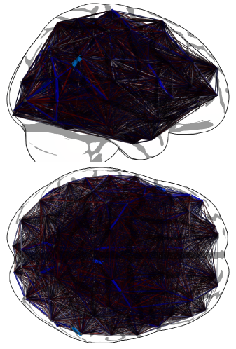
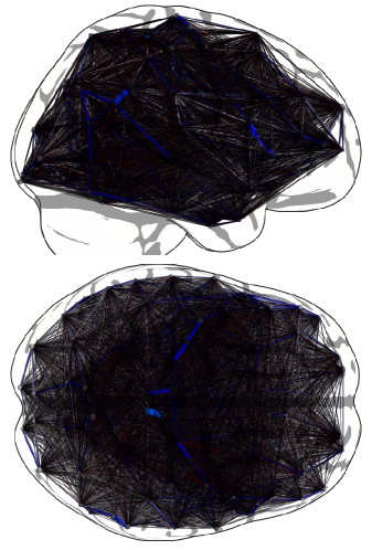
As can be seen from Figure 1, precision matrices corresponding to models that do not generalize well display a lot of background noise whereas in models that generalize well, a sparse structure stands out. Although an $\ell_{1}$ penalization is sparsity inducing, the optimal graphs estimated with such estimators are not very sparse (see table 1): a filling factor of 50% amounts to $5\,000$ edges. As a result, the corresponding graphs are not interpretable without thresholding (corresponding visualization are given in the supplementary materials). To interpret dense brain connectivity graphs, previous work relied on extracting a connectivity backbone using a maximal spanning tree [27], or graph statistics on thresholded adjacency matrices [2].

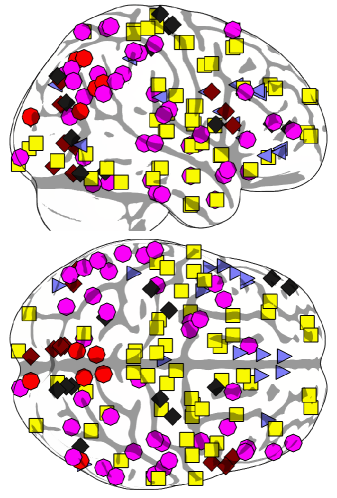
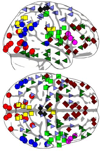
On the opposite, the $\ell_{21}$-penalized graph is very sparse, with only 700 edges. Adequate penalization serves as a replacement to backbone extraction; moreover it corresponds to a theoretically well-grounded and accurate model of brain connectivity. After embedding in 3D anatomical space, the estimated graph is very symmetric (see Figure 2). A third of the weight on the edges is on connections between a region and the corresponding one on the opposite hemisphere. In addition, the connectivity model displays strong fronto-parietal connections, while the visual system is globally singled out into one cluster, connected to the rest of the cortex mostly via the middle-temporal area.

Figure 1: Precision matrices computed with different estimators. The precision matrix is shown in false colors in the background and its support is shown in black and white in an inset.

5 An application: graph communities to describe functional networks

Even very sparse, high-dimensional functional connectivity graphs are hard to interpret. However, they are deemed of high neuroscientific interest, as their structure can reflect fundamental nervous system assembly principles. Indeed, there is evidence from the study of the fault-resilient structure of anatomical connections in the nervous systems that ensembles of neurones cluster together to form communities that are specialized to a cognitive task [5, 4, 27]. This process, known as functional integration goes along with a reduction of between-community connections, called segregation. So far, studies of full-brain connectivity graphs have focused on the analysis of their statistical properties, namely their small-world characteristics related to the emergence of strongly-connected communities in neural system. These properties can be summarized by a measure called modularity [4, 2, 28]. As the original measures introduced for integration and segregation are Gaussian entropy and mutual information measures [29, 30], the estimation of a well-conditioned Gaussian graphical model of the functional signal gives us an adequate tool to study large-scale modularity and integration in the brain. A limitation of the studies of statistical properties on graphs estimated from the data is that they may reflect properties of the estimation noise. Given that our graphical description generalizes well to unseen data, it should reflect the intrinsic properties of brain functional connectivity better than the sample correlation matrices previously used [4]. In this section, we study these properties on the optimal precision matrices describing a representative individual as estimated above.

Finding communities to maximize modularity

Graph communities are a concept originally introduced in social networks: communities are groups of densely-connected nodes with little between-group connections. Newman and Girvan [28] have introduced an objective function $Q$, called modularity, to measure the quality of a graph partition in a community structure. Choosing the partition to optimize modularity is a NP-hard problem, but Smyth and White formulate it as a graph partitioning problem, and give an algorithm [31] based on a convex approximation leading to spectral embedding and k-means clustering. The number of classes is chosen to optimize modularity.

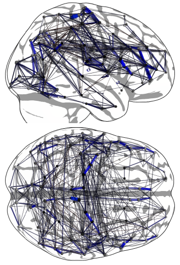
Full graph

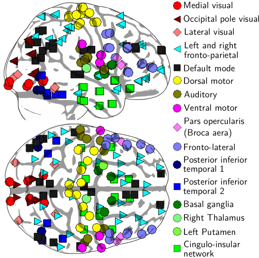
Communities

Figure 2: Functional-connectivity graph computed by $\ell_{21}$-penalized estimation and corresponding communities. The graph displayed on the left is not thresholded, but on the top view, connections linking one region to its corresponding one on the opposite hemisphere are not displayed.

Brain functional-connectivity communities

We apply Smyth and White’s algorithm on the brain connectivity graphs. We find that using the $\ell_{21}$-penalized precision matrices yields a higher number of communities, and higher modularity values (Table 1) then the other estimation strategies. We discuss in details the results obtained without regularization, and with the best performing regularization strategies: $\ell_{1}$ penalization on individual data, and $\ell_{21}$ penalization. The communities extracted from the sample precision matrix are mostly spread throughout the brain, while the graph estimated with $\ell_{1}$ penalization on individual data yields communities centered on anatomo-functional regions such as the visual system (figures in supplementary materials). The communities extracted on the $\ell_{21}$-penalized precision exhibit finer anatomo-functional structures, but also extract some known functional networks that are commonly found while studying spontaneous as well as task-related activity [3]. In Figure 2, we display the resulting communities, making use, when possible, of the same denominations as the functional networks described in [3]. In particular, the default mode network and the fronto-parietal network are structures reproducibly found in functional-connectivity studies that are non-trivial as they are large-scale, long-distance, and not comprised solely of bilateral regions.

$\ell_{1}$    $\ell_{21}$   

Figure 3: Between-communities integration graph obtained through $\ell_{1}$- (left) and $\ell_{21}$-penalization (right). The size of the nodes represents integration within a community and the size of the edges represents mutual information between communities. Region order is chosen via 1D Laplace embedding. The regions comprising the communities for the $\ell_{1}$-penalized graph are detailed in the supplementary materials.

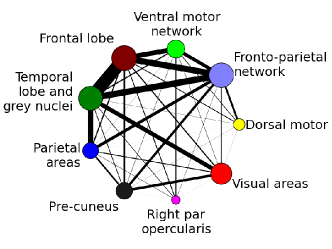
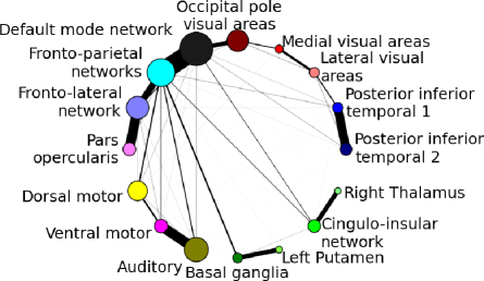
Integration and segregation in the graph communities

These functionally-specialized networks are thought to be the expression of integration and segregation processes in the brain circuits architecture. We apply the measures introduced by Tononi et al. [29] on the estimated graphs to quantify this integration and segregation, namely Gaussian entropy of the functional networks, and mutual information. However, following [32], we use conditional integration and conditional mutual information to obtain conditional pair-wise measures, and thus a sparser graph: for two sets of nodes $S_{1}$ and $S_{2}$,

Integration: $$I_{S_{1}} =\frac{1}{2}\log\det(\mathbf{K}_{S_{1}})$$ (4)

Mutual information: $$M_{S_{1},S_{2}} =I_{S_{1}\cup S_{2}}-I_{S_{1}}-I_{S_{2}},$$ (5)

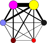
where $\mathbf{K}_{S_{1}}$ denotes the precision matrix restricted to the nodes in $S_{1}$. We use these two measures, pair-wise and within-community, to create a graph between communities.

This graph reflects the large-scale brain function organization. We compare the graph built using the $\ell_{1}$ and $\ell_{21}$-penalized precisions (figure 3). We find that the former is much sparser than the latter, reflecting a higher large segregation in between the communities estimated. The graph corresponding to the $\ell_{21}$ penalization segments the brain in smaller communities and care must be taken in comparing the relative integration of the different systems: for instance the visual system appears as more integrate on the $\ell_{1}$ graph, but this is because it is split in three on the $\ell_{21}$ graph.

Although this graph is a very simplified view of brain functional architecture at rest, it displays some of the key processing streams: starting from the primary visual system (medial visual areas), we can distinguish the dorsal visual pathway, going through the occipital pole to the intra-parietal areas comprised in the default mode network and the fronto-parietal networks, as well as the ventral visual pathway, going through the lateral visual areas to the inferior temporal lobe. The default mode and the fronto-parietal networks appear as hubs, connecting different networks with different functions, such as the visual streams, but also the motor areas, as well as the frontal regions.

6 Conclusion

We have presented a strategy to overcome the challenge of subject-to-subject variability and learn a detailed model of an individual’s full-brain functional connectivity using population data. The learnt graphical model is sparse and reveals the interaction structure between functional modules via conditional independence relationships that generalize to new data. As far as we can tell, this is the first time an unsupervised model of brain functional connectivity is backed by cross-validation. Also, from a machine learning perspective, this work is the first demonstration, to our knowledge, of joint estimation of multiple graphical models in a model-selection setting, and the first time it is shown to improve a prediction score for individual graphical models.

From a neuroscience perspective, learning high-dimensional functional connectivity probabilistic models opens the door to new studies of brain architecture. In particular, the models estimated with our strategy are well suited to exploring the graph-community structure resulting from the functional integration, specialization, and segregation of distributed networks. Our preliminary work suggests that a mesoscopic description of neural ensembles via high-dimensional graphical models can establish the link between the functional networks observed in brain imaging and the fundamental nervous-system assembly principles. Finally, subject-level Gaussian probabilistic models of functional connectivity between a few regions have proved useful for statistically-controlled inter-individual comparisons on resting-state, with medical applications [9]. Extending such studies to full-brain analysis, that have been so-far limited by the amount of data available on individual subjects, clears the way to new insights in brain pathologies [6, 8].

Supplementary materials

Full graph                                                             Between-communities                                      integration graph                                        Communities

Figure 4: Graph computed by maximum likelihood estimation on an individual subject’s data. The graph displayed is not thresholded, but on the top view, connections linking one region to its corresponding one on the opposite hemisphere are not displayed.

Full graph                      Communities

Figure 5: Graph computed by $\ell_{1}$-penalized estimation on an individual subject’s data. The graph displayed is not thresholded, but on the top view, connections linking one region to its corresponding one on the opposite hemisphere are not displayed.

References

- [1] M. Fox and M. Raichle: Spontaneous fluctuations in brain activity observed with functional magnetic resonance imaging. Nat Rev Neurosci 8 (2007) 700–711
- [2] E. Bullmore and O. Sporns: Complex brain networks: graph theoretical analysis of structural and functional systems. Nat Rev Neurosci 10 (2009) 186–198
- [3] S. Smith, et al. : Correspondence of the brain’s functional architecture during activation and rest. PNAS 106 (2009) 13040
- [4] S. Achard, et al. : A resilient, low-frequency, small-world human brain functional network with highly connected association cortical hubs. J Neurosci 26 (2006) 63
- [5] O. Sporns, et al. : Organization, development and function of complex brain networks. Trends in Cognitive Sciences 8 (2004) 418–425
- [6] G. Cecchi, et al. : Discriminative network models of schizophrenia. In: NIPS 22. (2009) 250–262
- [7] W. Seeley, et al. : Neurodegenerative Diseases Target Large-Scale Human Brain Networks. Neuron 62 (2009) 42–52
- [8] S. Huang, et al. : Learning brain connectivity of Alzheimer’s disease from neuroimaging data. In: Advances in Neural Information Processing Systems 22. (2009) 808–816
- [9] G. Varoquaux, et al. : Detection of brain functional-connectivity difference in post-stroke patients using group-level covariance modeling. In: IEEE MICCAI. (2010)
- [10] M. Greicius: Resting-state functional connectivity in neuropsychiatric disorders. Current opinion in neurology 21 (2008) 424
- [11] A. McLntosh and F. Gonzalez-Lima: Structural equation modeling and its application to network analysis in functional brain imaging. Human Brain Mapping 2(1) (1994) 2–22
- [12] J. Daunizeau, K. Friston, and S. Kiebel: Variational Bayesian identification and prediction of stochastic nonlinear dynamic causal models. Physica D 238 (2009)
- [13] J. Honorio and D. Samaras: Multi-Task Learning of Gaussian Graphical Models. In: ICML. (2010)
- [14] A. Dempster: Covariance selection. Biometrics 28(1) (1972) 157–175
- [15] O. Banerjee, et al. : Convex optimization techniques for fitting sparse Gaussian graphical models. In: ICML. (2006) 96
- [16] J. Duchi, S. Gould, and D. Koller: Projected subgradient methods for learning sparse gaussians. In: Proc. of the Conf. on Uncertainty in AI. (2008)
- [17] J. Friedman, T. Hastie, and R. Tibshirani: Sparse inverse covariance estimation with the graphical lasso. Biostatistics 9(3) (2008) 432–441
- [18] M. Yuan and Y. Lin: Model selection and estimation in regression with grouped variables. Journal-Royal Statistical Society Series B Statistical Methodology 68(1) (2006) 49
- [19] J. Guo, et al. : Joint estimation of multiple graphical models. Preprint (2009)
- [20] J. Chiquet, Y. Grandvalet, and C. Ambroise: Inferring multiple graphical structures. Stat and Comput (2010)
- [21] A. Rothman, et al. : Sparse permutation invariant covariance estimation. Electron J Stat 2 (2008) 494
- [22] O. Ledoit and M. Wolf: A well-conditioned estimator for large-dimensional covariance matrices. J. Multivar. Anal. 88 (2004) 365–411
- [23] C. F. Beckmann and S. M. Smith: Probabilistic independent component analysis for functional magnetic resonance imaging. Trans Med Im 23(2) (2004) 137–152
- [24] M. Perrot, et al. : Joint Bayesian Cortical Sulci Recognition and Spatial Normalization. In: IPMI. (2009)
- [25] M. Keller, et al. : Anatomically Informed Bayesian Model Selection for fMRI Group Data Analysis. In: MICCAI. (2009)
- [26] D. Cordes, et al. : Mapping functionally related regions of brain with functional connectivity MR imaging. American Journal of Neuroradiology 21(9) (2000) 1636–1644
- [27] P. Hagmann, et al. : Mapping the structural core of human cerebral cortex. PLoS Biol 6(7) (2008) e159
- [28] M. Newman and M. Girvan: Finding and evaluating community structure in networks. Phys rev E 69 (2004) 26113
- [29] G. Tononi, O. Sporns, and G. Edelman: A measure for brain complexity: relating functional segregation and integration in the nervous system. PNAS 91 (1994) 5033
- [30] O. Sporns, G. Tononi, and G. Edelman: Theoretical neuroanatomy: relating anatomical and functional connectivity in graphs and cortical connection matrices. Cereb Cortex 10 (2000) 127
- [31] S. White and P. Smyth: A spectral clustering approach to finding communities in graphs. In: 5th SIAM international conference on data mining. (2005) 274
- [32] D. Coynel, et al. : Conditional integration as a way of measuring mediated interactions between large-scale brain networks in functional MRI. In: Proc. ISBI. (2010)