Detection of brain functional-connectivity difference in post-stroke patients using group-level covariance modeling
Abstract
Functional brain connectivity, as revealed through distant correlations in the signals measured by functional Magnetic Resonance Imaging (fMRI), is a promising source of biomarkers of brain pathologies. However, establishing and using diagnostic markers requires probabilistic inter-subject comparisons. Principled comparison of functional-connectivity structures is still a challenging issue. We give a new matrix-variate probabilistic model suitable for inter-subject comparison of functional connectivity matrices on the manifold of Symmetric Positive Definite (SPD) matrices. We show that this model leads to a new algorithm for principled comparison of connectivity coefficients between pairs of regions. We apply this model to comparing separately post-stroke patients to a group of healthy controls. We find neurologically-relevant connection differences and show that our model is more sensitive that the standard procedure. To the best of our knowledge, these results are the first report of functional connectivity differences between a single-patient and a group and thus establish an important step toward using functional connectivity as a diagnostic tool.
1 Introduction
The correlation structure of brain activity, measured via fMRI, reveals stable inter-subject networks of distant brain regions that can be the expression of cognitive function. In particular, some connectivity networks are present in the absence of stimuli. They can reveal intrinsic brain activity and are studied in the resting-state paradigm. These structures are of particular interest to study and diagnose brain diseases and disorders [1] as they can be used for deep probes of brain function on diminished subjects. Not only can they extract medically or cognitively relevant markers on subjects unconscious [2], or with limited cooperation [3], but they also give information on higher-level cognitive systems that are challenging to probe via medical imaging or behavioral clinical tests [4].
To use functional connectivity as a quantitative inference tool, principled probabilistic comparison of connectivity structures across subjects is needed. Unlike with stimuli-response studies used routinely in functional neuroimaging, this comparison is challenging, as the underlying description of the signal is multivariate: each brain-activity time course is considered relative to others. Univariate group models, such as random effects or mixed effects, are in general not sound as they neglect the strong statistical dependence between parameters estimated from the data. Multivariate techniques have been successfully employed to single out outlying subjects [5], but have met little success: their results are difficult to interpret as they do not point to specific localized differences.
In this paper, we focus on the description of brain functional-connectivity using inter-regions correlation matrices. We first review the current practice in inter-subject functional covariance comparison and recall some results on the manifold of covariance matrices. Then, we introduce a probabilistic model at the group level for the different subjects’ correlation matrices, and a corresponding algorithm to detect connectivity differences in a specific parametrization of the covariance matrices, as correlations are a form of covariance. We quantify on simulated data the performance of this detection. Finally, we apply the model to the individual comparison of the connectivity structure of stroke patients to a group of healthy controls, and show that it outperforms the current practice.
2 State of the art
2.1 Problem statement: comparing functional brain connectivity
We consider subjects, represented by the correlation matrices between brain-activity time series extracted from ROIs: . The challenge is to give a probabilistic description of the population of correlation matrices so as to find the significant differences between subjects or groups. The current practice in functional-connectivity studies is to compare the coefficients of the correlation matrices across subjects (see for instance [3, 6]). This procedure can be expressed as a univariate additive linear model on the correlation matrix:
| (1) |
where is a covariance matrix representative of the mean effect, or the group, and encode subject-specific contributions.
However, with this description it is difficult to isolate significant contributions to . Indeed, for interpretation, some coefficients are zeroed out, eg by thresholding a test statistic, as in [3], which eventually leads to a non positive definite matrix, for which it is impossible to write a multivariate normal likelihood. As a result, the subject-variability description learned on a population cannot give probabilistic tests on new subjects.
2.2 Recent developments on the covariance-matrix manifold
The mathematical difficulty stems from the fact that the space of SPD matrices, , does not form a vector space: . The Fisher information matrix of the multivariate normal distribution can be used to construct a metric on a parametrization of covariance matrices [7] and thus define as a Riemannian manifold that is well-suited for performing statistics on covariances [8]. Local differences on this manifold can be approximated by vectors of the tangent space: if is close enough to , the application: maps locally the bipoint to , the space of symmetric matrices111Note that we do not use the same definition of the mapping as in [8, 7], as we are interested in mapping to , the tangent space around , and not the tangent space in . It extracts a statistically independent parametrization (Eq. (3) and (4)).. A convenient parametrization of is that forms an orthonormal basis of the tangent space [8]. Finally, gives the intrinsic norm of on the manifold, according to the metric around point : the distance between and in the manifold.
3 Matrix-variate random effects model for covariances
Multi-subject probability distribution for covariance matrices
Using the Riemannian parametrization of , we describe the individual correlation matrix population as a distribution of matrices scattered around a covariance matrix representative of the group, . As this distribution must be estimated with a small number of observations compared to the feature space, we model it using the probability density function that minimizes the information with a given mean on the manifold, the generalized Gaussian distribution [8]:
| (2) |
where encodes an isotropic variance on the manifold and is a normalization factor. Given multiple observations of corresponding to individual correlation matrices, , the maximum likelihood estimate of is independent of and given by the Fréchet mean of the observations [8], minimizing .
Parametrization in the tangent space
We express the individual covariance matrices as a perturbation of the group covariance matrix :
| (3) | |||||
| thus, using (2), | (4) |
The parameters of follow a normal distribution, with diagonal covariance , and the maximum-likelihood estimate of is given by . The model can thus be interpreted as a random-effect model on the parametrization of , in the space tangent to the manifold . Assuming that the distribution is narrow on the manifold, , eq. (3) can be seen as the application of the placement function to move a noise isotropic around to (see [8], section 3.5):
| (5) |
Model estimation from the data
We start from individual time-series of brain activity in selected regions of interest, . We use the Ledoit-Wolf shrinkage covariance estimator [9] for a good bias-variance compromise when estimating correlation matrices from time points with . From this estimate of individual correlation matrices, we compute the intrinsic mean on using algorithm 3 of [10]. Finally, we estimate from the residuals of individual correlation matrices in the space tangent in (see algorithm 1).
4 Testing pair-wise correlations statistics
The multivariate probabilistic model for correlations between regions exposed above enables us to define an average correlation matrix of a group, as well as the dispersion of the group in the covariance matrix space. Thus it can be used to test if a subject is different to a control group. However, to aid diagnosis, it is paramount to pin-point why such a subject may be different. In the tangent space, the parameters of are mutually independent. We can thus conduct univariate analysis on these parameters to test which significantly differs from the control group. However, the independence of the parameters is true only in the space tangent at the population average , of which we only have an estimate . Thus, to account for projection error, we resort to non-parametric sampling of the control population to define a null distribution for the parameters .
Specifically, we are interested in testing if a difference observed for a subject in one of the can be explained by variation of the control population. As the control population is typically small, we generate the null distribution by leave one out: for each control subject, we generate surrogate control populations by bootstrap from the other control subjects and estimate the corresponding average covariance . We use to project all the individual correlation matrices, including the left out subject, to compute , and we do a one sample T test of the difference between for the left out subject with regards to the resampled control group . We record the values of this T test as an estimate of the null distribution of the T test on the corresponding coefficient between the controls and a patient. Finally, we estimate the average covariance for the complete group of controls and, for each patient to investigate, we perform a T test of the difference between for the patient and the control group. We use to associate a p-value to each coefficient per subject. We correct for multiple comparisons using Bonferroni correction: for each patient, tests are performed. The procedure is detailed in algorithm 2.
5 Algorithm evaluation on simulated data
Algorithm 2 relies on approximations of the exact problem for coefficient-level detection of differences. In order to quantify the performance of this detection, we study Receiver Operator Characteristic (ROC) on simulated data: we draw a population of control covariances using eq. (5) with the parameters of normally distributed with deviation . For simulated patients, we add differences of amplitude to a few coefficients () of this variability noise. For and , we use the parameters estimated on real data (section 6). We investigate the performance of algorithm 2 to recover these differences for a variety of parameters. We observe good recovery for (Fig 1), and find that the comparison in the tangent space (eq. 5) outperforms a comparison in (eq. 1).
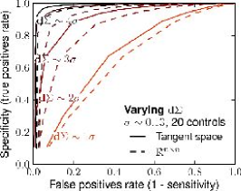
(a) 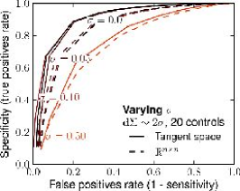 (b)
(b) 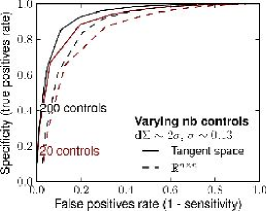 (c)
(c)
6 Application to post-stroke connectivity reorganization
Standard clinical scores, such as the NIHSS, as well as fMRI studies can be used to assess the consequences of cerebral strokes, but they test specific cognitive functions and have little sensitivity to higher-order cognitive malfunctions. Resting-state functional-connectivity is thus a valuable tool to study post-stroke reorganization. We apply our model to stroke patients.
Resting-state fMRI dataset
After giving informed consent, ischemic-stroke patients, as well as age-matched healthy controls, underwent MRI scanning. Subjects with existing neurology, psychiatry, or vascular pathologies were excluded from the study. 10 patients and 20 controls were scanned during a resting-state task: subjects were given no other task than to stay awake but keep their eyes closed. 2 sessions of 10 minutes of fMRI data were acquired on a Siemens 3T Trio scanner (245 EPI volumes, TR=2.46 s, 41 slices interlaced, isotropic 3 mm voxels). After slice-timing, motion correction, and inter-subject normalization using SPM5, 33 ROIs were defined in the main resting-state networks by intersecting a segmentation of the gray matter with correlation maps from seeds selected from the literature. For each subject, the BOLD time series corresponding to the regions were extracted and orthogonalized with respect to confound time series: time courses of the white matter and the cerebro-spinal fluid, and movement regressors estimated by the motion-correction algorithm. Covariance modeling was performed on the resulting 33 time series.
Separating patients from controls with the matrix-variate covariance model.
To measure the discriminative power of the matrix-variate model introduced in section 3, we test the likelihood of patient data in a model learned on controls. Specifically, we evaluate by leave one out the likelihood of each control in the model learned on the other controls. We compare this value to the average likelihood of patients in the 20 models obtained by leave one out. We perform this comparison both using the group model isotropic on the tangent space (eq. 5), and the group model isotropic in (eq. 1). We find that the model in the tangent space separates better patients from controls (Fig 2).
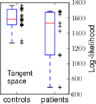
(a) 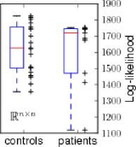 (b)
(b) 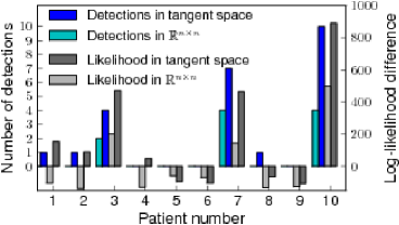 (c)
(c)
Detected connection differences
We apply algorithm 2 to detect the significant coefficient-level differences for each subject. We compare to a similar univariate procedure applied to the parametrization in given by eq. (1), rather than the tangent space. We find that coefficient-level analysis detects more differences between ROI pairs when applied on the tangent-space parametrization (Fig 2c).
(a) 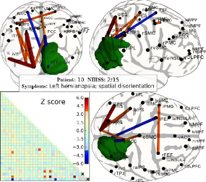 (b)
(b)
7 Discussion
Interpretation of the tangent space
Projecting on the space tangent to the group mean corresponds to applying a whitening matrix learned on the group (eq. 5) that converts the Gaussian process described by the group covariance to an independent and identically distributed (iid) process. In other words, the coloring of the time series common to the group is canceled out to compare subjects on iid coefficients on the correlation matrix.
Probing neurological processes
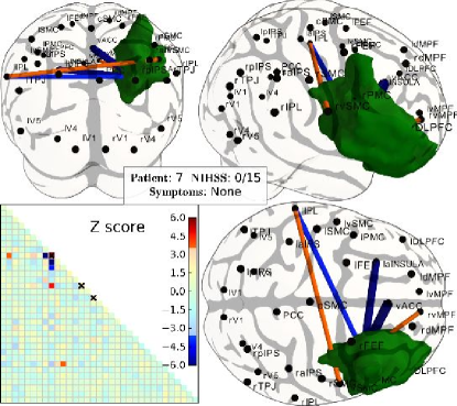
For certain subjects, both procedures fail to detect a single connection that makes a significant difference. Indeed, the variability of resting-state activity in the control group induces some variability in the projection to the tangent space. For patients with small lesions, this variability is larger than the univariate differences. On the other hand, for patients with important lesions, the functional connectivity analysis reveals profound differences in the correlation structure that reflect functional reorganization. Some express a direct consequence of the lesion, for example when the gray matter in one of two ROIs has been damaged by the lesion, as can be seen on Fig 3a. Others reflect functional reorganization. For instance, patient 10 has a right visual cortex damaged by a focal lesion, but the analysis shows increased connectivity in his left visual cortex (Fig 3b). Functional connectivity analysis thus reveals modifications that go beyond the direct anatomical consequences of the lesion.
8 Conclusion
We have presented a matrix-variate probabilistic model for covariances, and have shown that it can be expressed as a random effect model on a particular parametrization of the covariance matrix. The ability to draw conclusions on the connectivity between pairs of regions is important because it is a natural representation of the problem. We applied this model to the comparison of functional brain connectivity between subjects. We were able to detect significant differences in functional connectivity between a single stroke patient and 20 controls. A controlled detection of network-wide functional-connectivity differences between subjects opens the door to new markers of brain diseases as well as new insights in neuroscience, as functional connectivity can probe phenomena that are challenging to access via stimuli-driven studies.
References
- [1] M. Greicius: Resting-state functional connectivity in neuropsychiatric disorders. Current opinion in neurology 21 (2008) 424
- [2] A. Vanhaudenhuyse, et al. : Default network connectivity reflects level of consciousness in non-communicative brain-damaged patients. Brain 133 (2010) 161
- [3] D. Fair, et al. : Development of distinct control networks through segregation and integration. PNAS 104 (2007) 13507
- [4] L. Uddin and V. Menon: The anterior insula in autism: Under-connected and under-examined. Neuroscience and Biobehavioral Reviews 33 (2009) 1198–1203
- [5] J. Sato, et al. : An fMRI normative database for connectivity networks using one-class support vector machines. Human brain mapping 30 (2008) 1068
- [6] M. Rocca, et al. : Altered functional and structural connectivities in patients with MS: a 3-T study. Neurology 69 (2007) 2136
- [7] C. Lenglet, et al. : Statistics on the manifold of multivariate normal distributions: Theory and application to diffusion tensor MRI processing. Journal of Mathematical Imaging and Vision 25 (2006) 423–444
- [8] X. Pennec, P. Fillard, and N. Ayache: A Riemannian framework for tensor computing. International Journal of Computer Vision 66 (2006) 41–66
- [9] O. Ledoit and M. Wolf: A well-conditioned estimator for large-dimensional covariance matrices. J. Multivar. Anal. 88 (2004) 365–411
- [10] P. Fletcher and S. Joshi: Riemannian geometry for the statistical analysis of diffusion tensor data. Signal Processing 87 (2007) 250–262