CMB Lensing Reconstruction in Real Space

Abstract

We explore the reconstruction of the gravitational lensing field of the cosmic microwave background in real space showing that very little statistical information is lost when estimators of short range on the celestial sphere are used in place of the customary estimators in harmonic space, which are nonlocal and in principle require a simultaneous analysis of the entire sky without any cuts or excisions. Because virtually all the information relevant to lensing reconstruction lies on angular scales close to the resolution scale of the sky map, the gravitational lensing dilatation and shear fields (which unlike the deflection field or lensing potential are directly related to the observations in a local manner) may be reconstructed by means of quadratic combinations involving only very closely separated pixels. Even though harmonic space provides a more natural context for understanding lensing reconstruction theoretically, the real space methods developed here have the virtue of being faster to implement and are likely to prove useful for analyzing realistic maps containing a galactic cut and possibly numerous small excisions to exclude point sources that cannot be reliably subtracted.

I Introduction

Recently there has been much discussion of how the intervening mass from clustered matter between the last scattering surface (at $z\approx 1100$) and an observer at the present time distorts the CMB anisotropy by means of gravitational lensing blanchard ; cole ; tomita ; bernardeau ; van-waerbeke . On the level of the two-point correlation function, this effect distorts the TT (temperature-temperature) correlation power spectrum seljak and mixes the EE and BB polarization power spectra as well as distorting them zald ; benabed-bis ; seljak-ter . Lensing also introduces non-Gaussianities that manifest themselves in the higher-point correlation functions zaldarriaga ; cooray-ter . At the level of the three-point correlation function, to leading order there is no nonzero expectation value if we regard the lensing potential as a random field cooray ; kesden . However if we consider the CMB lensing potential as fixed, we find that expectation values of the form

$$\left<T(\boldsymbol{\theta})T(\boldsymbol{\theta}^{\prime})\right>_{\Phi(\boldsymbol{\theta}^{\prime\prime})}$$ (1)

do not vanish, and this property may be exploited to recover or “reconstruct” the lensing field using estimators quadratic in $T$ (or in $E$ and $B$) hu2001a .

Much effort has been devoted to developing an optimal reconstruction of the lensing potential in harmonic space, which implicitly assumes full sky coverage with no galactic cut, no bad pixels due to point sources that must be excised, and no nonuniform weighting to account for uneven sky coverage challinor ; lesgourgues ; bode . For a reconstruction based on the temperature anisotropy alone, it has been shown how to construct the optimal quadratic estimator in this idealized context hu2001b , and the improvement that can be gained from using an even more optimal maximum likelihood estimator is marginal seljak-bis , because the distortion due to lensing is small compared to the intrinsic cosmic variance and noise of the experiment (although this assumption is less valid at very large $\ell$ for very clean maps where the lensing signal is dominant). For the exploitation of polarized anisotropies, the situation is somewhat more complicated. When the experimental noise is large compared to the B polarization mode generated by lensing, the situation is essentially the same as for a reconstruction using the temperature data hu-okamoto ; cooray-bis . However at a higher sensitivity where the B signal is essentially entirely due to lensing, the quadratic estimator underperforms because the actual multipole moments rather than their averages should be used for the optimal weighting. In this case, the higher order corrections to the quadratic estimator present in the maximum likelihood estimator are no longer negligible hirata-seljak .

In this paper we investigate a real space approach to lensing reconstruction. Under the ideal conditions often assumed and described above, this approach would naturally yield the same result as the conventional approach in harmonic space. Our interest however lies in considering slightly non-optimal estimators that have been modified to have a finite range so that cuts, excisions of pixels, and non-uniform coverage may be included in a simple and flexible way. We believe that such non-ideal but more robust local estimators defined in real space may prove superior for confronting the complications inherent in analyzing real data smith ; miller ; perotto . Another advantage of the approach here is that the dilatation and pure shear provide separate and essentially independent lensing reconstructions which may be confronted with each other. This feature may prove useful as a way of diagnosing spurious signals, which are unlikely to affect the two reconstructions in the same way. Moreover the presence of two shear components enables one to estimate the noise of the reconstruction through the implied transverse displacement field, which is forbidden in weak lensing.

Before proceeding to the details of this program, it is useful to consider the relation between the various descriptions of the lensing and the deformation of the anisotropies in real space. It is also useful to consider which angular scales contribute the most statistical weight to the lensing reconstruction.

The lensing distortion of the CMB anisotropy on the surface of last scatter may be described in three ways: by a lensing potential $\Phi,$ by a deflection field $\boldsymbol{\xi}=\nabla\Phi,$ or by the three components of the shear tensor

$$\kappa=\begin{pmatrix}\kappa_{0}+\kappa_{+}&\kappa_{\times}\cr\kappa_{\times}&\kappa_{0}-\kappa_{+}\cr\end{pmatrix}=\nabla_{a}\nabla_{b}\Phi.$$ (2)

Even if we have simultaneous access to the entire sky, the descriptions $\Phi$ and $\boldsymbol{\xi}$ suffer from an ambiguity. $\Phi$ cannot be distinguished from $\Phi+\textrm{(constant)}$ and the vector field $\boldsymbol{\xi}$ can be measured only up to a constant translation (or more properly a rotation in the presence of sky curvature). This is because if we know only the CMB power spectrum, a patch of sky and its translation necessarily have the same likelihood on account of isotropy of the underlying stochastic process. Consequently, the absolute translation due to lensing cannot be observed. By contrast, locally the shear and dilatation (which are gradients of the translation vector field) are completely well defined. This can easily be seen by considering the effect of a constant deformation described by a deformation matrix $S$ relating the angular coordinates $\boldsymbol{\theta},$ the actual coordinates on the celestial sphere of a point on the last scattering surface, to the coordinates $\boldsymbol{\theta}^{\prime}$, the coordinates that the same point would have in the absence of lensing. We have $\boldsymbol{\theta^{\prime}}=S\boldsymbol{\theta}$ where $S=\exp[-\boldsymbol{\kappa}].$ (Note that we employ the flat sky approximation and assume that the deformation is small so that a linear treatment is adequate.) To linear order, the power spectrum is modified in the following way by this linear deformation, which preserves the homogeneity but not the isotropy of the underlying statistical process:

$$C(|{\boldsymbol{\ell}}|)\to C(\ell)\biggl{[}1+\kappa_{0}\left(\frac{d(\ln[C(\ell)])}{d(\ln[\ell])}+2\right)+\left(\frac{\kappa_{+}(\ell_{1}^{2}-\ell_{2}^{2})+\kappa_{\times}(2\ell_{1}\ell_{2})}{\ell^{2}}\right)\frac{d(\ln[C(\ell)])}{d(\ln[\ell])}\biggr{]}.$$ (3)

For the case of perfect scale invariance (i.e., a power law of the form $C(\ell)\propto\ell^{-2}$) there is no change in the correlations due to the dilatation component of $S,$ and similarly for a perfect white noise spectrum (i.e., a power law of the form $C(\ell)\propto\ell^{0}$) there is no sensitivity to the pure shear components $\kappa_{+}$ and $\kappa_{\times}$ in the anisotropic $(m=\pm 2)$ correlations.

To the extent that the shear-dilatation components are slowly varying, we may construct estimators of $\kappa_{0},$ $\kappa_{+},$ and $\kappa_{\times}$ as follows

$$\hat{\kappa}_{0} = {N_{0}}^{-1}\int_{A}d^{2}\theta~{}\int_{A}d^{2}\theta^{\prime}~{}\left[T(\boldsymbol{\theta})~{}T(\boldsymbol{\theta}^{\prime})-\left<T({\boldsymbol{\theta}})~{}T({\boldsymbol{\theta}^{\prime}})\right>_{\kappa=0}\right]$$ (5)

$$\times\int\frac{d^{2}\ell}{(2\pi)^{2}}\exp[i{\boldsymbol{\ell}}\cdot({\boldsymbol{\theta}}-{\boldsymbol{\theta}^{\prime}})]~{}\frac{C(\ell)}{[C(\ell)+N(\ell)]^{2}}\left(\frac{d(\ln[C(\ell)])}{d(\ln[\ell])}+2\right)$$

$$= {N_{0}}^{-1}{\cal A}^{-1}\int_{A}d^{2}\theta~{}\int_{A}d^{2}\theta^{\prime}~{}\left[T({\boldsymbol{\theta}})~{}T({\boldsymbol{\theta}^{\prime}})-\left<T({\boldsymbol{\theta}})~{}T({\boldsymbol{\theta}^{\prime}})\right>_{\kappa=0}\right]K_{0}({\boldsymbol{\theta}}-{\boldsymbol{\theta}^{\prime}})$$ (6)

$$= \frac{1}{\cal A}\int_{A}d^{2}\theta~{}\left[T({\boldsymbol{\theta}})~{}({\cal F}_{\kappa_{0}}T)({\boldsymbol{\theta}})-\textrm{(constant)}\right]$$ (7)

and similarly

$$\begin{pmatrix}\hat{\kappa}_{+}\cr\hat{\kappa}_{\times}\cr\end{pmatrix} = {N_{+,\times}}^{-1}\int_{A}d^{2}\theta~{}\int_{A}d^{2}\theta^{\prime}~{}T(\boldsymbol{\theta})~{}T({\boldsymbol{\theta}^{\prime}})~{}$$ (9)

$$\times\int\frac{d^{2}\ell}{(2\pi)^{2}}\exp[i{\boldsymbol{\ell}}\cdot({\boldsymbol{\theta}}-{\boldsymbol{\theta}^{\prime}})]~{}\frac{C(\ell)}{[C(\ell)+N(\ell)]^{2}}\frac{d(\ln[C(\ell)])}{d(\ln[\ell])}\begin{pmatrix}\cos(2\vartheta)\cr\sin(2\vartheta)\cr\end{pmatrix}$$

$$= {N_{+,\times}}^{-1}{\cal A}^{-1}\int_{A}d^{2}\theta~{}\int_{A}d^{2}\theta^{\prime}~{}T({\boldsymbol{\theta}})~{}T({\boldsymbol{\theta}^{\prime}})~{}\begin{pmatrix}K_{+}({\boldsymbol{\theta}}-{\boldsymbol{\theta}^{\prime}})\cr K_{\times}({\boldsymbol{\theta}}-{\boldsymbol{\theta}^{\prime}})\cr\end{pmatrix},$$ (10)

where the normalization factors are given by

$$N_{0} = {\cal A}\int\frac{d^{2}\ell}{(2\pi)^{2}}\frac{[C(\ell)]^{2}}{[C(\ell)+N(\ell)]^{2}}\left(\frac{d(\ln[C(\ell)])}{d(\ln[\ell])}+2\right)^{2},$$ (11)

$$N_{+} = N_{\times}=\frac{\cal A}{2}\int\frac{d^{2}\ell}{(2\pi)^{2}}\frac{[C(\ell)]^{2}}{[C(\ell)+N(\ell)]^{2}}\left(\frac{d(\ln[C(\ell)])}{d(\ln[\ell])}\right)^{2}$$ (12)

and ${\cal A}$ is the area of the domain. Here $N(\ell)$ is the noise of the experiment being considered and serves as a cut-off at large $\ell,$ above which there is very little exploitable information because of the low signal-to-noise of the CMB maps.

The above expressions assume a spatially flat, two-dimensional domain formally of large but finite area subject to a spatially uniform linear deformation. We may consider a toroidal domain in the limit that the periods of the torus become arbitrarily large (though the toroidal domain is not essential for the application of the real space estimator presented in this paper). Before proceeding it is useful to consider the relation of this simplified problem to the real problem of reconstructing the lensing field starting from a CMB map of finite resolution. Because of the smallness of the lensing distortion of the CMB anisotropy, the idealized situation considered above is less different from the actual situation, where one is dealing with a curved sky and a varying dilatation and shear fields, than one might at first sight suppose.

Figure 1: Lensing power spectrum. The lensing field power spectrum is shown represented in several manners. The three panels (from left to right) illustrate the lensing field expressed as potential, a deflection field, and dilatation/shear field, respectively. Plotted are $[\ell(\ell+1)C_{XX}/(2\pi)]^{1/2}$ where $XX=\Phi\Phi,$ ${\boldsymbol{\xi\xi}},$ $\kappa\kappa.$ Here $C_{\ell}^{\boldsymbol{\xi\xi}}=\ell(\ell+1)~{}C_{\ell}^{\Phi\Phi},$ and $C_{\ell}^{\kappa\kappa}=\ell^{2}(\ell+1)^{2}~{}C_{\ell}^{\Phi\Phi}/4.$ Of the three, the last power spectrum is more directly related to the observed distortion.

The rightmost panel of Fig. 1 shows the shear-dilatation power spectrum as a function of multipole number $\ell,$ and we observe that for $\ell<100,$ the distortion is always less than about $1.5\%.$ This implies that in order to attain an $(S/N)$ of approximately unity it is necessary to consider a region containing at least $O(10^{3})$ resolution elements, where a resolution element is a pixel of the map of sufficient size so that the noise and angular resolution of the survey give $S/N\approx 1.$ Consequently, there is little point to trying to reconstruct the lensing field over a region not having at least 30 resolution elements on a side. If the distortion from lensing were greater, the situation would be different.

For the ideal linear estimator

$$\frac{1}{\sigma^{2}_{\hat{\kappa}_{0,ideal}}}=\left(\frac{S}{N}\right)^{2} = \sum_{\ell,m}\frac{C_{\ell}^{2}}{2(C_{\ell}+N_{\ell})^{2}}\left[\frac{d(\ln[C])}{d(\ln[\ell])}+2\right]^{2}$$ (13)

$$\approx \frac{{\cal A}}{(4\pi)}\int_{0}^{\infty}d\ell~{}\ell~{}\frac{C(\ell)^{2}}{(C(\ell)+N(\ell))^{2}}\left[\frac{d(\ln[C(\ell)])}{d(\ln[\ell])}+2\right]^{2}$$ (14)

where ${\cal A}$ is the area of the sky patch considered.

We now consider other unbiased estimators of $\kappa_{0}$ and $\kappa_{+}$ where a slight increase in the variance is compensated for by other desirable properties. We are presently interested in estimators for which the real space filtering kernel is short range. To this end it is useful to define the inner product on the space of weight vectors ${w}=\{w_{\ell}\}$:

$$\left<w^{A},w^{B}\right> = \sum_{\ell,m}\frac{1}{2(C_{\ell}+N_{\ell})^{2}}w^{A}_{\ell,m}w^{B}_{\ell,m}$$ (15)

$$= {\cal A}\int\frac{d^{2}\ell}{(2\pi)^{2}}\frac{1}{2[C(\ell)+N(\ell)]^{2}}w^{A}(\boldsymbol{\ell})w^{B}(\boldsymbol{\ell})$$ (16)

where we give both the spherical and flat sky continuum forms. If we set $w_{ideal}(\ell)=\delta C(\ell)_{th,\kappa_{0}=1}=C(\ell)[\frac{d\ln C_{\ell}}{d\ln\ell}+2],$ then in terms of the above inner product

$$\hat{\kappa}_{0,ideal}=\frac{\left<w_{ideal},\delta C_{obs}\right>}{\left<w_{ideal},w_{ideal}\right>}$$ (17)

and

$$\left(\frac{S}{N}\right)^{2}_{\kappa_{0},ideal}=\left<\delta C_{th,\kappa_{0}=1},\delta C_{th,\kappa_{0}=1}\right>.$$ (18)

Given an arbitrary weight vector $w,$ using the above inner product we may define the following unbiased estimator of $\kappa_{0}$

$$\hat{\kappa}_{0}(w)=\frac{\left<w,\delta C_{obs}\right>}{\left<w,w_{ideal}\right>}$$ (19)

provided that the denominator does not vanish, and its variance is given by $\left<w,w\right>/\left<w_{ideal},w\right>^{2},$ so that the increase in variance with respect to the ideal estimator is given by following geometric expression for the secant squared

$$\frac{\textrm{Var}(\hat{\kappa}_{0}(w))}{\textrm{Var}(\hat{\kappa}_{0}(w_{ideal}))}=\frac{\left<w,w\right>\left<w_{ideal},w_{ideal}\right>}{\left<w,w_{ideal}\right>^{2}}~{}\rm{sec}^{2}(\chi).$$ (20)

For $\kappa_{+}$ and $\kappa_{\times}$ analogous formulae may be derived straightforwardly.

Figure 2: Character of the signal. The top row shows as a function of multipole number $\ell$ the temperature power spectrum and local spectral index, defined as $d\ln C_{\ell}/d\ln\ell,$ for the standard cosmology (WMAP best-fit model). On the bottom row, the left panel shows the normalized cumulative $\chi^{2}$ as a function of $\ell$ integrated both from the left and from the right using the sensitivity and resolution parameters for the PLANCK experiment (where the 100, 143 and 217 GHz channels have been combined in quadrature) bluebook . We observe that the central 80% of the information is concentrated in the range $\ell=800$–$1600.$ Smaller $\ell$ contribute almost no information because there are comparatively very few independent multipoles, and moreover the angular spectrum in the sky is very nearly scale invariant. At much larger $\ell$ instrument noise and beam smearing wash out the usable signal. In the intermediate range a structure of plateaus connected by steep rises can be observed. This structure is a direct result of the Doppler oscillations. Around the crests and troughs the spectrum is almost scale invariant and hence does not contain any information for determining the dilatation. The right panel shows the corresponding plot for the shear, where the plateaus are less pronounced.

We consider how the information (or $S^{2}/N^{2}$) contained in the ideal estimator is distributed over the various multipoles. In Fig. 2 [panels (c) and (d)] we plot the quantity

$$F_{<}(\bar{\ell})=\frac{\int_{0}^{\bar{\ell}}\ell~{}d\ell~{}\frac{{C(\ell)}^{2}}{({C(\ell)}+{N(\ell)})^{2}}\left[\frac{d(\ln[C(\ell)])}{d(\ln[\ell])}+2\right]^{2}}{\int_{0}^{\infty}\ell~{}d\ell~{}\frac{{C(\ell)}^{2}}{({C(\ell)}+{N(\ell)})^{2}}\left[\frac{d(\ln[C(\ell)])}{d(\ln[\ell])}+2\right]^{2}}$$ (21)

and $F_{>}(\bar{\ell})=1-F_{<}(\bar{\ell})$ where

$$N_{\ell}=N_{0}~{}\exp\left[+\ell^{2}\theta^{2}_{beam}\right]=N_{0}~{}\exp\left[+\ell^{2}/\ell^{2}_{beam}\right]$$ (22)

and $\ell_{beam}=(810)(10^{\prime}/\theta_{beam}^{fwhm}).$ The corresponding quantity is also shown for the shear.

In their present state, the ideal minimum variance kernels for the estimators $\hat{\kappa}_{0},$ $\hat{\kappa}_{+},$ and $\hat{\kappa}_{\times}$ have their support sharply peaked at small separations, but nevertheless there is still some small support for large separation. We now investigate how much information is lost if the support at large separation is completely cut away. The quantitative way to characterize this loss is to ask by what factor the variance of the estimator is increased relative to the optimal estimator after our pruned estimator has been renormalized to render it unbiased.

In real space the minimum variance full-sky estimator kernel for $\kappa_{0}$ is given by

$$K_{ideal}(\theta) = \int_{0}^{\infty}\ell~{}d\ell~{}K_{ideal}(\ell)$$ (23)

$$= \int_{0}^{\infty}\ell~{}d\ell~{}{J_{0}(\ell\theta)}\frac{1}{N_{ideal}}\frac{C(\ell)}{[C(\ell)+N(\ell)]^{2}}~{}\left[\frac{d(\ln[C(\ell)])}{d[\ln(\ell)]}+2\right].$$ (24)

This kernel may be inverted using the following inverse Bessel transform:

$$K_{ideal}(\ell)=\frac{1}{2\pi}\int_{0}^{\infty}\theta~{}d\theta~{}J_{0}(\ell\theta)~{}K_{ideal}(\theta).$$ (25)

We limit the support of the kernel by requiring that $K(\theta)$ be nonzero only for $\theta\leq\theta_{max}$ where $\theta_{max}$ is varied. This is accomplished numerically by expressing $J_{0}(\ell\theta)$ as a linear combination of cubic spline basis functions spanning the interval $\theta\in[0,\theta_{max}]$ and optimizing for the shape that minimizes the variance calculated according to eqn. (20). Analogous expressions may be obtained for the shear by replacing $J_{0}$ with $J_{2}.$ Fig. 3 shows the variance ratio as a function of $\theta_{max}$ for the dilatation and shear estimators. We observe that the increase in variance at small separations is more modest for the shear estimator.

Figure 3: Performance of estimator with truncated angular support. We indicate how limiting the angular support of the filter in our estimator increases the noise. The panels on the top row refer to the dilatation filter, while the panels on the bottom row refer to the shear filter. Panel (a) indicates how the estimator variance (with the estimator normalized to be unbiased) increases as the angular support (disk radius in degrees) is reduced. Panels (b) and (c) indicate the profiles of the optimal truncated estimators in both angular space and harmonic space.

II Results: Dilatation and Shear Reconstruction

In the previous section we showed how by means of a linear filter ${\cal F}_{\kappa_{0}}$ applied to a temperature map $T(\boldsymbol{\theta}),$ we may obtain a reconstructed dilatation field through the product map

$$\kappa_{0,rec}(\boldsymbol{\theta})=T(\boldsymbol{\theta})({\cal F}_{\kappa_{0}}T)(\boldsymbol{\theta})-c$$ (26)

where $c$ is a constant offset. We presented a theoretical derivation of the optimal shape for such a filter. The best shape for the filter depends both on the cosmological model, and more importantly on the details of the experiment, because most of the statistical weight is situated on the smallest angular scales, near the resolution limit of the experiment. If the primordial anisotropies dominated to arbitrarily small scales and experiments of unlimited sensitivity and angular resolution were possible, the lensing field could be reconstructed as accurately as desired simply by increasing the angular resolution and sensitivity. For a given experiment, the desirable filter shape may be intuitively understood as follows. We assume weak lensing (i.e., $|\kappa|\ll 1).$ We want to measure the change in shape of the power spectrum (or rather of the “local” power spectrum within a certain finite size patch for the case of interest of a non-uniform dilatation). Working in the flat sky approximation, which is appropriate because the length scales most sensitive to the changes in overall scale are small (i.e., $\ell\gg 100),$ we define ${\cal C}(\ell)=\ell^{2}~{}C(\ell).$ Under a small dilatation, which transforms the temperature map as follows

$$T(\boldsymbol{\theta})\to T(\boldsymbol{\theta}^{\prime})=T\Bigl{(}\exp[-\kappa]~{}\boldsymbol{\theta}\Bigr{)},$$ (27)

the power spectrum transforms as

$${\cal C}(\ell)\to{\cal C}\Bigl{(}\exp[+\kappa]~{}\ell\Bigr{)},$$ (28)

so for positive dilatations the power spectrum in the form ${\cal C}(\ell)$ squeezes to the left in such a way that the amplitudes of the various features remain unchanged. If the dilatation is small, the change in the power spectrum is proportional to $\kappa~{}{\cal C}^{\prime}(\ell).$ To make a good filter for implementing the above scheme giving the reconstruction with the least noise, we wish to block modes of wavenumber where ${\cal C}(\ell)$ is approximately flat, to allow modes of wavenumber where ${\cal C}(\ell)$ is rising to pass with a positive phase factor, and to allow modes of wavenumber where ${\cal C}(\ell)$ is falling to pass with a negative phase factor. Moreover the filter should combine the different wavenumbers according to inverse variance weighting in order to minimize the noise of the reconstructed dilatation field.

The quality of the inverse variance reconstruction may be characterized quantitatively in terms of the variance of the reconstructed field. We define a quality factor $Q$ so that

$$(\delta\kappa)^{2}\approx\frac{Q}{\cal A}$$ (29)

where ${\cal A}$ is the area of the region over which the reconstructed field has been averaged and $(\delta\kappa)$ is the fluctuation in $\kappa$ averaged over that same area. Here $Q$ is equal to $\sigma^{2}_{\hat{\kappa}_{0}}/{\cal A}$ where $\sigma^{2}_{\hat{\kappa}_{0}}$ is given in eqn. (14).

Implicit is the assumption that the noise in the reconstructed dilatation field lacks long range correlations—that is, it can be treated as white noise beyond a certain angular coherence scale. This is indeed the case because the filter ${\cal F}_{\kappa_{0}}$ blocks small wave numbers. We assume that the area ${\cal A}$ is sufficiently large so that the white noise regime has been reached.

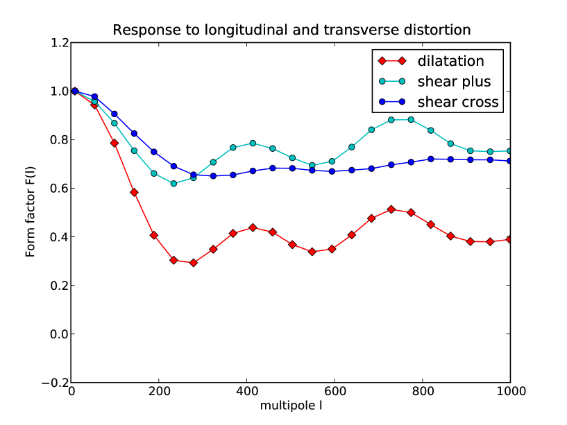
Figure 4: Estimator form factors at large lensing wave numbers. We plot as a function of multipole number the form factors for the dilatation, longitudinal shear, and cross shear reconstructions using the filter described in the text. Noise for the Planck instrument combining the 100+143+217 GHz channels is assumed using bluebook values and combining channels in the naive way bluebook . A deformation field whose wavenumber constitutes the horizontal axis was applied to unlensed maps. For the dilatation and the “plus” shear, a longitudinal displacement field was used. For the “cross” shear a transverse deformation was applied. As a result of symmetry considerations, the responses of the dilatation and plus shear to a transverse deformation have vanishing expectation values (i.e., they are pure noise) and hence are not shown. The same holds for the cross shear response to a longitudinal deformation.

For a non-uniform dilatation field having a small wavenumber, the previous analysis carries over with very small corrections. Using the same filter as for the uniform case, one expects that

$$\left<\kappa_{0,recon}(\boldsymbol{\theta})\right>=\kappa_{0,exact}(\boldsymbol{\theta}),$$ (30)

in other words, that there is negligible bias. However for larger wavenumbers a form factor appears due to the fact that our estimator probes the power spectrum over a window of a finite width in angular space, and consequently smoothes the underlying exact dilatation field thus reducing its amplitude. Quantitatively, if the dilatation field has the form

$$\kappa_{0}\cos(\boldsymbol{\ell}\cdot\boldsymbol{\theta}+\phi),$$ (31)

the expectation value of the reconstructed field takes the form

$$F(\ell)\kappa_{0}\cos(\boldsymbol{\ell}\cdot\boldsymbol{\theta}+\phi)$$ (32)

and as before the noise field will have the same statistics. $F(\ell)$ is known as the form factor and satisfies $F(0)=1.$ $F(\ell)$ falls off for increasing $\ell,$ eventually going to zero. The form factors are indicated in Fig. 4. The shear plus estimator experiences less smoothing than the dilatation estimator because the form of the $\ell$-space filter has less cancellations as can be seen in Fig. 3.

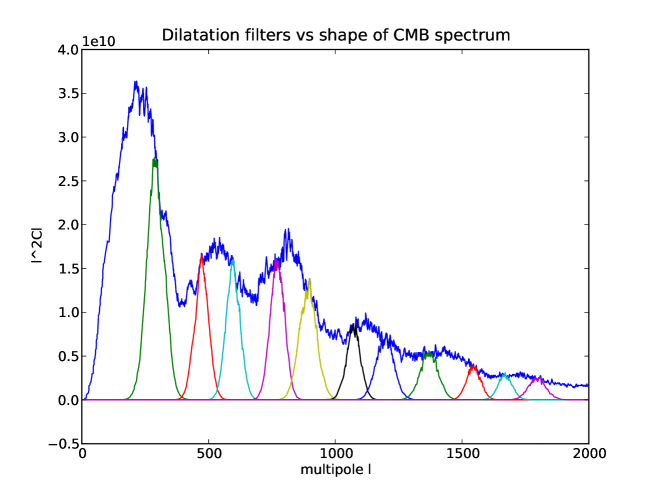
In Fig. 5 we present an alternative, more heuristic derivation of the dilatation field reconstruction filter which has the virtue of rendering manifest the contribution of various features in the power spectrum to the reconstruction. This alternative filter is a combination of Gaussian filters placed at the locations in multipole space where the magnitude of the derivative of $\ell^{2}~{}C(\ell)$ is greatest, and whose widths are chosen to correspond roughly to the width of the rise and fall of this quantity. In Table 1 the $(S/N)^{2}$ for each of these filters are shown and we indicate their relative statistical weights as well as the $(S/N)^{2}$ when they are combined using inverse variance weighting. Somewhat surprisingly, this naive derivation yields a filter almost as efficient as the optimal one.

Figure 5: Alternative filter derivation. We generate a dilatation reconstruction filter by an alternate procedure whereby Gaussian filters are placed at the locations in multipole space where the magnitude of the derivative of $\ell^{2}~{}C(\ell)$ is greatest. The widths of the filters are chosen to correspond roughly to the width of the rise and fall of this quantity.

$\ell_{center}$	$\sigma_{\ell}$	$\left(S/N\right)^{2}$ $\deg^{-2}\cdot\kappa_{0}^{-2}$
$300$	50	$3.13\pm 0.26$
$470$	40	$1.56\pm 0.13$
$600$	40	$3.02\pm 0.25$
$770$	40	$0.13\pm 0.01$
$900$	50	$61.51\pm 5.02$
$1070$	40	$1.44\pm 0.12$
$1200$	50	$30.66\pm 2.50$
$1370$	50	$23.24\pm 1.90$
$1550$	40	$42.53\pm 3.47$
Combined		$167.22\pm 13.65$
Ideal		$140.50\pm 11.47$

Table 1: Performance of individual feature filters. The first nine entries correspond to Gaussian filters whose centers and widths are indicated and have been placed where the features of the power spectrum change the most in response to a small dilatation. The last column expresses the sensitivity of each filter. The next-to-last row shows $(S/N)^{2}$ resulting when the filters are combined using inverse covariance weighting. This is compared to the ideal filter. The errors result from Monte Carlo noise.

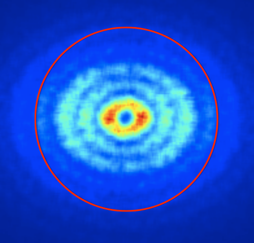
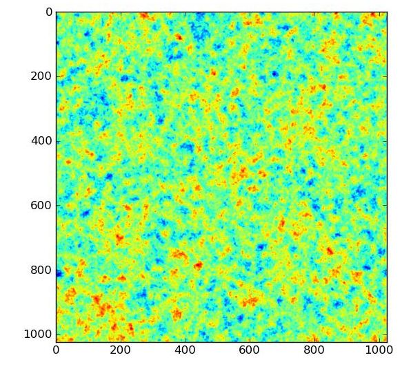
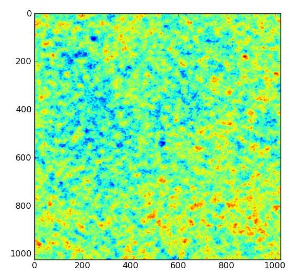
Figure 6: Distortion of power spectrum due to shear. In the two-dimensional plot in harmonic space the power spectrum is shown after a pure shear transformation has been applied turning the sequences of acoustic peaks into concentric ellipses rather than concentric circles. In the real space images (middle, unlensed and right, sheared) the transformation is hardly apparent to the unaided eye.

We now repeat the same analysis for a constant pure shear deformation, for concreteness with $\kappa_{+}>0,$ $\kappa_{\times}=0,$ there is a stretching along the $x$-direction with the same amount of compression along the $y$-direction, so that the temperature map is deformed according to

$$T(\theta_{x},\theta_{y})\to T^{\prime}(\theta_{x}^{\prime},\theta_{y}^{\prime})=T(e^{-\kappa_{+}}\theta_{x},e^{+\kappa_{+}}\theta_{y}),$$ (33)

and for the harmonic coefficients one has the following transformation law

$$T(\ell_{x},\ell_{y})\to T^{\prime}(\ell_{x}^{\prime},\ell_{y}^{\prime})=T(e^{+\kappa_{+}}\ell_{x},e^{-\kappa_{+}}\ell_{y}).$$ (34)

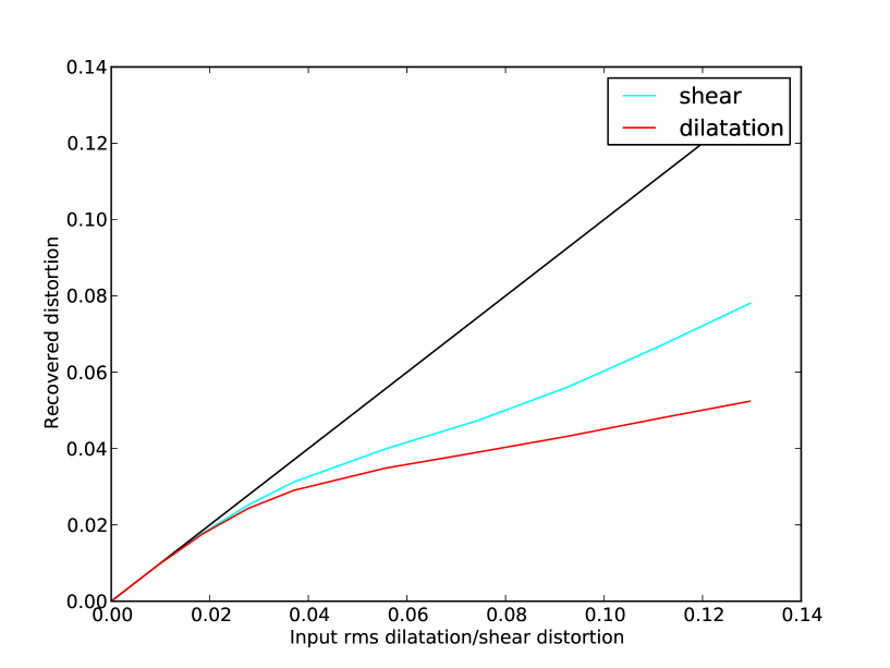
For any power spectrum having a shape like that of the CMB temperature, where at all wavenumbers the spectrum is “red” compared to a white noise spectrum, a pure shear deformation causes a loss of power for wavevectors oriented close to the stretched principal axis and a corresponding increase of power for wavevectors close to the principal axis of compression. Along the diagonal direction the power is unaffected. The estimator developed in the first section of this paper exploits this anisotropy to reconstruct two components of the shear field. The effect is illustrated in Fig. 6. In panel (a) the acoustic oscillations, which would in the absence of lensing be visible as a series of concentric circular rings, have as a result of a pure shear deformation been deformed into concentric ellipses. Panels (b) and (c) show simulated temperature maps before and after a constant shear deformation, here exaggerated in magnitude (with $\kappa_{0}=0.1$) for clarity. One observes that the annuli become elliptical. Unlike for the dilatation field, where a scale-invariant spectral index implies that statistically the pattern does not change, for pure shear an isotropic scale invariant random field is deformed into an anisotropic scale invariant random field, where heuristically one might say that the series of elliptical (rather than on the average circular) diffuse motifs have been put down in a scale-free manner. In Fig. 7 we show the extent of the region of linear response of the dilatation and shear estimators. Ignoring higher order terms gives rise to a bias which can be corrected seljak-bis ; kesden_2003 .

Figure 7: Estimator non-linearity. We plot the recovered root-mean-square distortion versus the input root-mean-square distortion in order to characterize the range of linear response for our estimator. The input is a long-wavelength longitudinal deformation, so that the two-dimension shear and dilatation are exactly half the one-dimensional dilatation. Exactly the same non-linearity will plague the quadratic estimator as well, since the two have been demonstrated to be equivalent at low wavenumber (as discussed in section IV).

III Combining the $\kappa_{0}(\theta),$ $\kappa_{+}(\theta)$ and $\kappa_{\times}(\theta)$ reconstructions

In the previous two sections we have shown how by means of three filters ${\cal F}_{\kappa_{0}},$ ${\cal F}_{\kappa_{+}},$ and ${\cal F}_{\kappa_{\times}}$ we may obtain a noisy reconstruction of the fields $\kappa_{0}(\boldsymbol{\theta}),$ $\kappa_{+}(\boldsymbol{\theta}),$ and $\kappa_{\times}(\boldsymbol{\theta})$ in real space. We also saw how the reconstruction was essentially finite-range in real space and could be made of compact support with very little loss of information relative to the optimal nonlocal, full-sky reconstruction. The reconstructed fields are not independent but related according to the following relations

$$\kappa_{0}(\boldsymbol{\ell}) = -\frac{1}{2}(\ell_{x}^{2}+\ell_{y}^{2})\Phi(\boldsymbol{\ell}),$$ (35)

$$\kappa_{+}(\boldsymbol{\ell}) = -\frac{1}{2}(\ell_{x}^{2}-\ell_{y}^{2})\Phi(\boldsymbol{\ell}),$$ (36)

$$\kappa_{\times}(\boldsymbol{\ell}) = -\ell_{x}\ell_{y}\Phi(\boldsymbol{\ell}),$$ (37)

which are local in harmonic space. These consistency relations, expressed in terms of the lensing potential $\Phi,$ can be used to harmonize the reconstruction. Even though there are three reconstructed fields, the cross shear, which would result from a transverse deformation that cannot be produced by weak lensing, is pure noise. The noises present in the longitudinal shear and the dilatation reconstruction are uncorrelated because one involves the $m=0$ sector and the other the $m=\pm 2$ sector. Harmonization by inverse variance weighting reduces the noise. If we consider the noise in the reconstruction field to lowest order in the perturbation expansion (as 4-point functions of the underlying Gaussian field) ignoring higher-order terms, then there are no correlations between reconstructed fields components of differing wavenumber. Consequently, in order to obtain the lowest noise estimator of $\Phi,$ it suffices to consider each $\boldsymbol{\ell}$ sector separately and to use the covariance matrix of the noise in $\kappa_{0}(\boldsymbol{\ell}),$ $\kappa_{+}(\boldsymbol{\ell}),$ and $\kappa_{\times}(\boldsymbol{\ell})$ as a basis for the optimal harmonization.

IV Comparison with the quadratic estimator

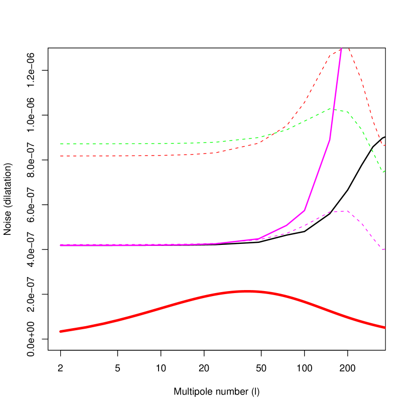
In this section we show how the dilatation and shear estimators developed in this paper are related to the linearly optimal quadratic estimator for the lensing field hu2001a ; hu2001b . We demonstrate that in the low-$\ell$ limit the quadratic estimator becomes a linear combination of our dilatation and longitudinal shear estimators. In fact in this limit the linearly optimal quadratic estimator is identical to the inverse variance weighted linear combination of the dilatation and longitudinal shear estimators, whose noises are uncorrelated. At higher $\ell,$ the approximation used to derive this relation progressively breaks down. To quantify this degradation, we plot in Fig. 8 the increase in variance of the combined dilatation plus longitudinal shear estimators. For the reasons already presented concerning the minute statistical weight contributed by small multipoles, we find it adequate to work in the flat sky approximation.

The relation in real space (valid to linear order)

$$\delta T(\boldsymbol{\theta})=\nabla\Phi(\boldsymbol{\theta})\cdot\nabla T(\boldsymbol{\theta})$$ (38)

in harmonic space translates into

$$\delta T(\boldsymbol{\ell})=\int\frac{d^{2}\ell^{\prime}}{(2\pi)^{2}}(-\boldsymbol{\ell}^{\prime})\cdot(\boldsymbol{\ell}-\boldsymbol{\ell}^{\prime})~{}\Phi(\boldsymbol{\ell}^{\prime})~{}T(\boldsymbol{\ell}-\boldsymbol{\ell}^{\prime})$$ (39)

where we define

$$\left<T(\boldsymbol{\ell})T(\boldsymbol{\ell}^{\prime})\right>=(2\pi)^{2}\delta^{2}(\boldsymbol{\ell}+\boldsymbol{\ell}^{\prime})~{}C(\ell).$$ (40)

Since $T_{sky}=T+\delta T,$ it follows that to leading (linear) order

$$\left<T_{sky}\left(\frac{\boldsymbol{\ell}^{\prime}}{2}+\boldsymbol{\ell}\right)T_{sky}\left(\frac{\boldsymbol{\ell}^{\prime}}{2}-\boldsymbol{\ell}\right)\right>$$ (41)

$$= \Phi(\boldsymbol{\ell}^{\prime})\times\left[-\left(\frac{\boldsymbol{\ell}^{\prime}}{2}-\boldsymbol{\ell}\right)\cdot\boldsymbol{\ell}^{\prime}~{}C\left(\left|\boldsymbol{\ell}-\frac{\boldsymbol{\ell}^{\prime}}{2}\right|\right)-\left(\frac{\boldsymbol{\ell}^{\prime}}{2}+\boldsymbol{\ell}\right)\cdot\boldsymbol{\ell}^{\prime}~{}C\left(\left|\boldsymbol{\ell}+\frac{\boldsymbol{\ell}^{\prime}}{2}\right|\right)\right].$$ (42)

It follows that

$$\hat{\Phi}(\boldsymbol{\ell}^{\prime})=N^{-1}\sum_{\boldsymbol{\ell}}W(\boldsymbol{\ell}^{\prime};\boldsymbol{\ell})~{}T_{sky}\left(\frac{\boldsymbol{\ell}^{\prime}}{2}+\boldsymbol{\ell}\right)~{}T_{sky}\left(\frac{\boldsymbol{\ell}^{\prime}}{2}-\boldsymbol{\ell}\right)$$ (43)

is the minimum variance unbiased estimator for the Fourier coefficient $\Phi(\boldsymbol{\ell}^{\prime})$ where

$$W(\boldsymbol{\ell}^{\prime};\boldsymbol{\ell})=\frac{\left[-\left(\frac{\boldsymbol{\ell}^{\prime}}{2}-\boldsymbol{\ell}\right)\cdot\boldsymbol{\ell}^{\prime}~{}C\left(\left|\boldsymbol{\ell}-\frac{\boldsymbol{\ell}^{\prime}}{2}\right|\right)-\left(\frac{\boldsymbol{\ell}^{\prime}}{2}+\boldsymbol{\ell}\right)\cdot\boldsymbol{\ell}^{\prime}~{}C\left(\left|\boldsymbol{\ell}+\frac{\boldsymbol{\ell}^{\prime}}{2}\right|\right)\right]}{\left[C\left(\boldsymbol{\ell}-\frac{\boldsymbol{\ell}^{\prime}}{2}\right)+N\left(\boldsymbol{\ell}-\frac{\boldsymbol{\ell}^{\prime}}{2}\right)\right]\left[C\left(\boldsymbol{\ell}+\frac{\boldsymbol{\ell}^{\prime}}{2}\right)+N\left(\boldsymbol{\ell}+\frac{\boldsymbol{\ell}^{\prime}}{2}\right)\right]}$$ (44)

and

$$N=\sum_{\boldsymbol{\ell}}\frac{\left[-\left(\frac{\boldsymbol{\ell}^{\prime}}{2}-\boldsymbol{\ell}\right)\cdot\boldsymbol{\ell}^{\prime}~{}C\left(\left|\boldsymbol{\ell}-\frac{\boldsymbol{\ell}^{\prime}}{2}\right|\right)-\left(\frac{\boldsymbol{\ell}^{\prime}}{2}+\boldsymbol{\ell}\right)\cdot\boldsymbol{\ell}^{\prime}~{}C\left(\left|\boldsymbol{\ell}+\frac{\boldsymbol{\ell}^{\prime}}{2}\right|\right)\right]^{2}}{\left[C\left(\boldsymbol{\ell}-\frac{\boldsymbol{\ell}^{\prime}}{2}\right)+N\left(\boldsymbol{\ell}-\frac{\boldsymbol{\ell}^{\prime}}{2}\right)\right]\left[C\left(\boldsymbol{\ell}+\frac{\boldsymbol{\ell}^{\prime}}{2}\right)+N\left(\boldsymbol{\ell}+\frac{\boldsymbol{\ell}^{\prime}}{2}\right)\right]}.$$ (45)

We may approximate the quantity in the square brackets in eqn. (42) to linear order to obtain

$$-\left(\frac{\boldsymbol{\ell}^{\prime}}{2}-\boldsymbol{\ell}\right)\cdot\boldsymbol{\ell}^{\prime}~{}C\left(\left|\boldsymbol{\ell}-\frac{\boldsymbol{\ell}^{\prime}}{2}\right|\right)-\left(\frac{\boldsymbol{\ell}^{\prime}}{2}+\boldsymbol{\ell}\right)\cdot\boldsymbol{\ell}^{\prime}~{}C\left(\left|\boldsymbol{\ell}+\frac{\boldsymbol{\ell}^{\prime}}{2}\right|\right)$$ (46)

$$= -{\ell^{\prime}}^{2}~{}C(\ell)-(\boldsymbol{\ell}\cdot\boldsymbol{\ell}^{\prime})^{2}\frac{1}{\ell}\frac{\partial C(\ell)}{\partial\ell}$$ (47)

$$= -\frac{1}{2}\frac{{\ell^{\prime}}^{2}}{\ell^{2}}\frac{\partial[\ell^{2}C(\ell)]}{\partial\ln[\ell]}-\left(\frac{(\boldsymbol{\ell}\cdot\boldsymbol{\ell}^{\prime})^{2}-\frac{1}{2}{\ell^{\prime}}^{2}\ell^{2}}{\ell^{2}}\right)\frac{\partial[C(\ell)]}{\partial\ln[\ell]}$$ (48)

$$= -\frac{1}{2}{\ell^{\prime}}^{2}\left\{\frac{1}{\ell^{2}}\frac{\partial[\ell^{2}C(\ell)]}{\partial\ln[\ell]}+\cos[2\Theta]\frac{\partial[C(\ell)]}{\partial\ln[\ell]}\right\}$$ (49)

where $\Theta$ is the angle between $\boldsymbol{\ell}$ and $\boldsymbol{\ell}^{\prime}.$ The expression is remarkably similar to a linear combination of the expressions appearing in the dilatation and the pure shear reconstruction of the previous section.

Figure 8: Comparison with quadratic estimator We plot the noises of the various estimators compared to the expected signal (heavy red curve). The quadratic estimator is indicated in thick black. The dilatation and shear estimators are shown in dashed red and green, respectively, and when combined nominally give the dashed magenta curve, but when the imperfect overlap with the expected signal is taken into account, yield the solid magenta curve. The blue curve would be indicative of the actual noise in the recovered maps, but if the imperfect overlap where corrected to remove the bias at high $\ell$ the heavy magenta curve would result. For comparison we show the predicted lensing signal (as computed by CAMB for the WMAP best fit model) as the heavy red curve.

Approximating the numerator of (44) as (49) and the denominator of (44) as $[C(\ell)+N(\ell)]^{2},$ we may write the three estimators in the following unified manner:

$$\hat{D}(\boldsymbol{\ell}^{\prime}) = \frac{1}{2}\frac{\cal A}{N_{D}}\int\frac{d^{2}\ell}{(2\pi)^{2}}\frac{{[C(\ell)]}}{[C(\ell)+N(\ell)]^{2}}\left[\frac{\partial(\ln[\ell^{2}C(\ell)])}{\partial[\ln(\ell)]}\right]~{}T_{sky}\left(\frac{\boldsymbol{\ell}^{\prime}}{2}+\boldsymbol{\ell}\right)~{}T_{sky}\left(\frac{\boldsymbol{\ell}^{\prime}}{2}-\boldsymbol{\ell}\right)$$ (50)

$$\hat{S}_{L}(\boldsymbol{\ell}^{\prime}) = \frac{1}{2}\frac{\cal A}{N_{S_{L}}}\int\frac{d^{2}\ell}{(2\pi)^{2}}\frac{{[C(\ell)]}}{[C(\ell)+N(\ell)]^{2}}\left[\cos[2\Theta(\boldsymbol{\ell},\boldsymbol{\ell}^{\prime})]\frac{\partial(\ln[C(\ell)])}{\partial[\ln(\ell)]}\right]~{}T_{sky}\left(\frac{\boldsymbol{\ell}^{\prime}}{2}+\boldsymbol{\ell}\right)~{}T_{sky}\left(\frac{\boldsymbol{\ell}^{\prime}}{2}-\boldsymbol{\ell}\right)$$ (51)

$$\hat{Q}(\boldsymbol{\ell}^{\prime}) = \frac{1}{2}\frac{\cal A}{N_{Q}}\int\frac{d^{2}\ell}{(2\pi)^{2}}\frac{{[C(\ell)]}}{[C(\ell)+N(\ell)]^{2}}\left[\frac{\partial(\ln[\ell^{2}C(\ell)])}{\partial[\ln(\ell)]}+\cos[2\Theta(\boldsymbol{\ell},\boldsymbol{\ell}^{\prime})]\frac{\partial(\ln[C(\ell)])}{\partial[\ln(\ell)]}\right]$$ (53)

$$\qquad\times T_{sky}\left(\frac{\boldsymbol{\ell}^{\prime}}{2}+\boldsymbol{\ell}\right)~{}T_{sky}\left(\frac{\boldsymbol{\ell}^{\prime}}{2}-\boldsymbol{\ell}\right)$$

where

$$N_{D}(\boldsymbol{\ell}^{\prime}) = \frac{1}{2}{\cal A}\int\frac{d^{2}\ell}{(2\pi)^{2}}\frac{{[C(\ell)]}^{2}}{[C(\ell)+N(\ell)]^{2}}\left[\frac{\partial(\ln[\ell^{2}C(\ell)])}{\partial[\ln(\ell)]}\right]^{2}$$ (54)

$$N_{S_{L}}(\boldsymbol{\ell}^{\prime}) = \frac{1}{2}{\cal A}\int\frac{d^{2}\ell}{(2\pi)^{2}}\frac{{[C(\ell)]}^{2}}{[C(\ell)+N(\ell)]^{2}}\left[\cos[2\Theta(\boldsymbol{\ell},\boldsymbol{\ell}^{\prime})]\frac{\partial(\ln[C(\ell)])}{\partial[\ln(\ell)]}\right]^{2}$$ (55)

$$N_{Q}(\boldsymbol{\ell}^{\prime}) = \frac{1}{2}{\cal A}\int\frac{d^{2}\ell}{(2\pi)^{2}}\frac{{[C(\ell)]}^{2}}{[C(\ell)+N(\ell)]^{2}}\left[\frac{\partial(\ln[\ell^{2}C(\ell)])}{\partial[\ln(\ell)]}+\cos[2\Theta(\boldsymbol{\ell},\boldsymbol{\ell}^{\prime})]\frac{\partial(\ln[C(\ell)])}{\partial[\ln(\ell)]}\right]^{2}$$ (56)

and $N_{Q}=N_{D}+N_{S_{L}}$ because the cross term cancels under the integral.

The quantities $N_{D},$ $N_{S_{L}},$ $N_{Q}$ express the amount of information provided by the respective estimators, and we have shown that in the limit where $\boldsymbol{\ell}^{\prime}$ is small

$$\hat{Q}(\boldsymbol{\ell}^{\prime})=\frac{N_{D}(\ell^{\prime})}{N_{D}(\ell^{\prime})+N_{S_{L}}(\ell^{\prime})}\hat{D}(\boldsymbol{\ell}^{\prime})+\frac{N_{S_{L}}(\ell^{\prime})}{N_{D}(\ell^{\prime})+N_{S_{L}}(\ell^{\prime})}\hat{S}_{L}(\boldsymbol{\ell}^{\prime}).$$ (57)

The exact expressions in Fourier space for the dilatation and shear statistics at not necessarily small wavenumber $\boldsymbol{\ell}^{\prime}$ are

$$\hat{D}(\boldsymbol{\ell}^{\prime}) = \frac{{\cal A}}{2}{1\over N_{D}(\ell^{\prime})}\int\frac{d^{2}\ell}{(2\pi)^{2}}\left\{F\left(\frac{\boldsymbol{\ell}^{\prime}}{2}+\boldsymbol{\ell}\right)+F\left(\frac{\boldsymbol{\ell}^{\prime}}{2}-\boldsymbol{\ell}\right)\right\}~{}T_{sky}\left(\frac{\boldsymbol{\ell}^{\prime}}{2}+\boldsymbol{\ell}\right)~{}T_{sky}\left(\frac{\boldsymbol{\ell}^{\prime}}{2}-\boldsymbol{\ell}\right)~{}$$ (58)

$$\hat{S}_{L}(\boldsymbol{\ell}^{\prime}) = \frac{{\cal A}}{2}{1\over N_{S_{L}}(\ell^{\prime})}\int\frac{d^{2}\ell}{(2\pi)^{2}}\biggl{\{}G\left(\frac{\boldsymbol{\ell}^{\prime}}{2}+\boldsymbol{\ell}\right)\cos\left[2\Theta\left(\frac{\boldsymbol{\ell}^{\prime}}{2}+\boldsymbol{\ell},\boldsymbol{\ell}^{\prime}\right)\right]$$ (60)

$$\qquad\qquad+G\left(\frac{\boldsymbol{\ell}^{\prime}}{2}-\boldsymbol{\ell}\right)\cos\left[2\Theta\left(\frac{\boldsymbol{\ell}^{\prime}}{2}-\boldsymbol{\ell},\boldsymbol{\ell}^{\prime}\right)\right]\biggr{\}}~{}T_{sky}\left(\frac{\boldsymbol{\ell}^{\prime}}{2}+\boldsymbol{\ell}\right)~{}T_{sky}\left(\frac{\boldsymbol{\ell}^{\prime}}{2}-\boldsymbol{\ell}\right)~{}$$

where

$$F(\bar{\ell})=\frac{C(\bar{\ell})}{[C(\bar{\ell})+N(\bar{\ell})]^{2}}\frac{\partial(\ln[\bar{\ell}^{2}C(\bar{\ell})])}{\partial(\ln[\bar{\ell}])},$$ (61)

$$G(\bar{\ell})=\frac{C(\bar{\ell})}{[C(\bar{\ell})+N(\bar{\ell})]^{2}}\frac{\partial(\ln[C(\bar{\ell})])}{\partial(\ln[\bar{\ell}])}.$$ (62)

To express compactly the increase in variance due to the non-optimality for $\boldsymbol{\ell}^{\prime}$ away from zero, it is useful to define the inner product

$$\left<\hat{A},\hat{B}\right>=\frac{{\cal A}}{2}\int\frac{d^{2}\ell}{(2\pi)^{2}}(C+N)\left(\frac{\boldsymbol{\ell}^{\prime}}{2}+\boldsymbol{\ell}\right)(C+N)\left(\frac{\boldsymbol{\ell}^{\prime}}{2}-\boldsymbol{\ell}\right)A(\boldsymbol{\ell})B(\boldsymbol{\ell})$$ (63)

where

$$\hat{A}=\frac{{\cal A}}{2}{1\over N_{A}}\int\frac{d^{2}\ell}{(2\pi)^{2}}~{}A(\boldsymbol{\ell})~{}T_{sky}\left(\frac{\boldsymbol{\ell}^{\prime}}{2}+\boldsymbol{\ell}\right)~{}T_{sky}\left(\frac{\boldsymbol{\ell}^{\prime}}{2}-\boldsymbol{\ell}\right)~{}$$ (64)

and $\hat{B}$ is defined analogously.

In this notation the various estimators have the following shape functions:

$$Q(\boldsymbol{\ell};\boldsymbol{\ell}^{\prime}) = \frac{2}{(\ell^{\prime})^{2}}\frac{-\left(\frac{\boldsymbol{\ell}^{\prime}}{2}-\boldsymbol{\ell}\right)\cdot\boldsymbol{\ell}^{\prime}~{}C\left(\left|\boldsymbol{\ell}-\frac{\boldsymbol{\ell}^{\prime}}{2}\right|\right)-\left(\frac{\boldsymbol{\ell}^{\prime}}{2}+\boldsymbol{\ell}\right)\cdot\boldsymbol{\ell}^{\prime}~{}C\left(\left|\boldsymbol{\ell}+\frac{\boldsymbol{\ell}^{\prime}}{2}\right|\right)}{(C+N)\left(\frac{\boldsymbol{\ell}^{\prime}}{2}+\boldsymbol{\ell}\right)(C+N)\left(\frac{\boldsymbol{\ell}^{\prime}}{2}-\boldsymbol{\ell}\right)}$$ (65)

$$D(\boldsymbol{\ell},\boldsymbol{\ell}^{\prime}) = \frac{1}{2}\left\{F\left(\frac{\boldsymbol{\ell}^{\prime}}{2}+\boldsymbol{\ell}\right)+F\left(\frac{\boldsymbol{\ell}^{\prime}}{2}-\boldsymbol{\ell}\right)\right\},$$ (66)

$$S_{L}(\boldsymbol{\ell},\boldsymbol{\ell}^{\prime}) = \frac{1}{2}\Biggl{\{}G\left(\frac{\boldsymbol{\ell}^{\prime}}{2}+\boldsymbol{\ell}\right)\cos\left[2\Theta\left(\frac{\boldsymbol{\ell}^{\prime}}{2}+\boldsymbol{\ell},\boldsymbol{\ell}^{\prime}\right)\right]$$ (68)

$$\qquad+G\left(\frac{\boldsymbol{\ell}^{\prime}}{2}-\boldsymbol{\ell}\right)\cos\left[2\Theta\left(\frac{\boldsymbol{\ell}^{\prime}}{2}-\boldsymbol{\ell},\boldsymbol{\ell}^{\prime}\right)\right]\Biggr{\}}.$$

It follows that the increase in the variance is given by the following expression for the secant squared

$$\frac{\sigma^{2}(D)}{\sigma^{2}(Q)}=\frac{\left<\hat{Q},\hat{Q}\right>\left<\hat{D},\hat{D}\right>}{\left<\hat{Q},\hat{D}\right>^{2}}.$$ (69)

In Fig. 8 we indicate the performance of the several estimators at finite $\ell^{\prime}.$ We plot $C_{\ell}^{(\delta\kappa_{0})(\delta\kappa_{0})}$(i.e. the expectation value of the square modulus of the harmonic coefficient on the sphere for the reconstruction noise) for the estimators $Q,$ $D,$ and $S_{L},$ in black, dashed red and dashed green, respectively. The dashed magenta curve indicates the noise obtained by combining $D$ and $S_{L}$ using inverse variance weighting. The solid magenta curve indicates the correction when the lack of overlap is taken into account to render the estimator unbiased at large wavenumber. We assume an instrument noise combining the Planck 100+143+217 GHz channels according to the specifications given in the bluebook bluebook . At low wavenumber, $Q$ exhibits a flat (i.e., white noise) spectrum, which subsequently divergences at large $\ell^{\prime}.$ At very low $\ell^{\prime}$ we observe that the noise from $Q$ is the same as the noise from $D$ and $S_{L}$ combined in quadrature, as shown theoretically in the text, but at higher $\ell^{\prime}$ the approximations used break down and a noise excess is observed. We observe that for $\ell\mathrel{\raise 1.29167pt\hbox{$<$}\mkern-14.0mu\lower 2.58334pt\hbox{$\sim$}}70,$ the difference in performance between the estimator developed here and the linearly optimal quadratic estimator is minimal. At higher wavenumbers beyond $\ell\mathrel{\raise 1.29167pt\hbox{$>$}\mkern-14.0mu\lower 2.58334pt\hbox{$\sim$}}100,$ however, the variance increases rapidly due to lack of overlap with the ideal kernel. There is a priori no reason why a real space approach could not be extended to higher wavenumbers for the lensing field. However, in the present paper we do not explore how this would work.

V Concluding remarks

We have demonstrated how to reconstruct in real space using a filter of compact support the weak gravitational lensing field, here represented as three fields, a dilatation field $\kappa_{0}(\boldsymbol{\theta})$ and the two components of the pure shear distortion field $\kappa_{+}(\boldsymbol{\theta})$ and $\kappa_{\times}(\boldsymbol{\theta}).$ The three fields are related by a set of nonlocal consistency conditions, which may subsequently be exploited to reduce the noise of the reconstruction. Except for an integration constant and two translational and one rotational zero modes, the weak lensing may alternatively and equivalently be described by either (1) a gravitational lensing potential $\Phi(\boldsymbol{\theta}),$ (2) a displacement field ${\boldsymbol{\xi}}(\boldsymbol{\theta}),$ $\Phi(\boldsymbol{\theta}),$ (2) a displacement field ${\boldsymbol{\xi}(\boldsymbol{\theta})},$ or (3) the dilatation field $\kappa_{0}(\boldsymbol{\theta})$ and the two components of the pure shear distortion field $\kappa_{+}(\boldsymbol{\theta})$ and $\kappa_{\times}(\boldsymbol{\theta}).$ In this paper we argue that for the purpose of reconstruction the representation (3) is advantageous because this is the representation for which the lensing field bears a local relation to the real space CMB maps. This locality comes at a price because the three components are not independent and subject to nonlocal consistency conditions, which may be exploited to improve the reconstruction. Locality allows different regions of the sky to be analyzed independently in a natural way, quite unlike the quadratic reconstruction in harmonic space, where the entire sky must be analyzed simultaneously. This approach and variations thereof hold promise for dealing with partial sky coverage and excised point sources. For the filters developed in this paper there is very little loss of information for the lensing field at low wavenumbers. However at larger wavenumbers the lensing signal is attenuated according to a wavenumber dependent form factor, which can be deconvolved by applying a correction filter.

Acknowledgements: MB and KM acknowledge support from a joint CNRS/NRF travel grant. The work of MB, CSC and MR was supported in part by the Projet Blanc VIMS-PLANCK of the Agence Nationale de la Recherche. KM and CSC are supported by the South African National Research Foundation.

References

• (1) A. Blanchard & J. Schneider, “Gravitational lensing effect on the fluctuations of the cosmic background radiation,” A&A 184, 1 (1987)
• (2) Cole & G Eftstathiou, “Gravitational lensing of fluctuations in the microwave background radiation,” MNRAS 239, 195 (1989)
• (3) K. Tomita & K. Watanabe, “Gravitational Lens Effect on the Cosmic Background Radiation Due to Nonlinear Inhomogeneities,” Prog. Theor. Phys. 82, 563 (1989)
• (4) F. Bernardeau, “Weak lensing detection in CMB maps,” A&A 324, 15 (1997) (astro-ph/961101); F. Bernardeau, “Lens distortion effects on CMB maps,” A&A 338, 767 (1998) (astro-ph/9802243)
• (5) L. Van Waerbeke, F. Bernardeau & K. Benabed, “Lensing effect on the relative orientation between the cosmic microwave background ellipticities and the distant galaxies,” Ap. J. 540, 14 (2000) (astro-ph/9910366)
• (6) U. Seljak, “Gravitational lensing effect on cosmic microwave background anisotropies: a power spectrum approach,” Ap. J. 463, 1 (1996) (astro-ph/9505109)
• (7) U Seljak & M Zaldarriaga, “Signature of gravity waves in polarization of the microwave background,” Phys. Rev. Lett. 78, 2054 (1997) (astro-ph/9609169); M. Zaldarriaga & U Seljak, “Gravitational lensing effect on cosmic microwave background polarization,” Phys. Rev. D58, 023003 (1998) (astro-ph/9803150)
• (8) K. Benabed, F. Bernardeau & L. Van Waerbeke, “CMB B polarization to map the large scale structures of the universe,” Phys. Rev. D63, 043501 (2001) (astro-ph/0003038)
• (9) U. Seljak & C. Hirata, “Gravitational lensing as a contaminant of the gravity wave signal in CMB,” Phys. Rev. D69, 043005 (2004) (astro-ph/0310163)
• (10) M. Zaldarriaga, “Lensing of the CMB: Non-Gaussian Aspects,” Phys. Rev. D62, 063510 (2000) (astro-ph/9910498)
• (11) A. Cooray, “Weak lensing of the cosmic microwave background: Power spectrum covariance,” Phys. Rev. D65, 063512 (2002) (astro-ph/0110415)
• (12) A. Cooray & M. Kesden, “Weak lensing of the CMB: Extraction of lensing information from the trispectrum,” New Astron. 8, 231 (2003) (astro-ph/0204068)
• (13) M. Kesden, A. Cooray & M. Kamionkowski, “Weak lensing of the CMB: Cumulants of the probability distribution function,” Phys. Rev. D66, 083007 (2002) (astro-ph/0208325)
• (14) W. Hu, “Weak lensing of the CMB: a harmonic approach,” Phys. Rev. D62, 043007 (2000) (astro-ph/0001303)
• (15) A. Challinor & A. Lewis, “Lensed CMB power spectra from all-sky correlation functions,” Phys. Rev. D71 103010 (2005) (astro-ph/0502425); A. Challinor & A. Lewis, “Weak gravitational lensing of the CMB,” Phys. Rept. 429, 1 (2006) (astro-ph/0601594)
• (16) J. Lesgourgues, L. Perotto, S. Pastor & M. Piat, “Probing neutrino masses with CMB lensing extraction,” Phys. Rev. D73, 045021 (2006) (astro-ph/0511735)
• (17) S. Das & P. Bode, “A Large Sky Simulation of the Gravitational Lensing of the Cosmic Microwave Background,” (astro-ph/07113793)
• (18) W. Hu, “Mapping the dark matter through the CMB damping tail,” Ap.J. 557, L79 (2001) (astro-ph/0105424)
• (19) C. Hirata & U. Seljak, “Analyzing weak lensing of the cosmic microwave background using the likelihood function,” Phys. Rev. D67, 043001 (2003) (astro-ph/0209489)
• (20) W. Hu & T. Okamoto, “Mass reconstruction with CMB polarization,” Ap. J. 574, 566 (2002) (astro-ph/0111606)
• (21) A. Cooray, “Lensing reconstruction of primordial cosmic microwave background polarization,” Phys. Rev. D66, 103509 (2002) (astro-ph/0205306)
• (22) C.M. Hirata &U. Seljak, “Reconstruction of lensing from the cosmic microwave background polarization,” Phys. Rev. D68, 083002 (2003) (astro-ph/0306354)
• (23) PLANCK Collaboration, The Scientific Programme of PLANCK, ESA-SCI 1, 5 (2005) (arXiv:astro-ph/0604069)
• (24) K. Smith, O. Zahn & O. Dore, “Detection of Gravitational Lensing in the Cosmic Microwave Background,” Phys. Rev. D76, 043510 (2007) (astro-ph/0705.3980)
• (25) N. J. Miller, M. Shimon & B.G. Keating, “CMB Beam Systematics: Impact on Lensing Parameter Estimation,” (astro-ph/0806.3096)
• (26) L. Perotto, J. Bobin, S. Plaszczynski, J.-L. Starck & A. Lavabre, “Reconstruction of the CMB lensing for Planck,” (astro-ph/0903.1308)
• (27) M. Kesden, A. Cooray & M. Kamionkowski, “Lensing Reconstruction with CMB Temperature and Polarization,” Phys. Rev. D67, 123507 (2003) (astro-ph/0302536)