NLO QCD corrections to top quark pair production in association with one hard jet at hadron colliders

Abstract

We compute the QCD corrections to the production of a $t\bar{t}$ pair in association with one hard jet at the Tevatron and the LHC, using the method of generalized $D$-dimensional unitarity. Top quark decays are included at leading order in perturbative QCD. We present kinematic distributions of top quark decay products in lepton plus jets and dilepton final states at the Tevatron and the LHC, using realistic selection cuts. We confirm a strong reduction of the top quark forward-backward asymmetry in $p\bar{p}\to t\bar{t}j$ at next-to-leading order, first observed by Dittmaier, Uwer and Weinzierl. We argue that there is a natural way to understand this reduction and that it does not imply a breakdown of the perturbative expansion for the asymmetry.

1 Introduction

Experiments at the Large Hadron Collider (LHC) are in the process of testing the very successful paradigm of the past thirty years – the Standard Model of particle physics – in an entirely new energy regime. The goal of these experiments is to unravel the mechanism of electroweak symmetry breaking. Electroweak symmetry breaking may occur due to the Higgs mechanism, as in the Standard Model, or it may be a consequence of more complex dynamics. In the Standard Model the unusually large mass of the top quark is introduced by hand and top quarks do not play any role in electroweak symmetry breaking. This may change in extensions of the Standard Model. Moreover, the large mass of the top quark makes its interactions with an agent of electroweak symmetry breaking parametrically enhanced, relative to other quarks. Therefore, top quarks provide a window of opportunity to investigate physics of electroweak symmetry breaking; this motivates a rigorous experimental program to study top quarks and their properties.

More than a decade after the discovery of the top quark in 1995 [1, 2], the Tevatron remains at the forefront of top quark studies. During that time, CDF and D0 reached remarkable precision in measuring the top quark production cross-section in $p\bar{p}$ collisions and the top quark mass [3]. Also, the top quark charge is constrained by experimental measurements [4, 5] and the hypothesis that the top quark spin is one half follows indirectly from the $p\bar{p}\to t\bar{t}$ cross-section measurement and is consistent with the observation of the top quark decay $t\to Wb$. The structure and the strength of $tbW$ interaction vertex was thoroughly studied [6, 7] and limits on exotic contributions to top quark decays were placed. A recent measurement of the forward-backward asymmetry of the top quark [8, 9] may point towards non-standard contributions to top quark pair production; currently, such a possibility is being actively discussed.

In spite of the enormous integrated luminosity accumulated by the Tevatron, many of their measurements are limited by statistics since the ratio of the hadron center of mass collision energy to twice the top quark mass is not large. This will change with the start-up of the LHC since the LHC will be a $t\bar{t}$ factory. It is expected that many of the studies performed at the Tevatron will be continued and extended at the LHC with much higher statistics. The higher energy of the LHC leads to a much larger cross-section for the top quark pair production, compared to the Tevatron, and, also, to a greater variety of the kinematics of the produced top quarks. In contrast to the Tevatron, top quarks are produced with larger energies and transverse momenta at the LHC. This kinematic feature implies larger probability for top quarks to radiate gluons and the increase of the relative importance of the $t\bar{t}+{\rm jets}$ final state in the inclusive $t\bar{t}$ sample.

It is important to understand how many jets are produced in association with a $t\bar{t}$ pair. Indeed, since top quarks may decay into leptons, missing energy and jets, $t\bar{t}$ production is an important background to standard signatures of physics beyond the Standard Model, where the number of jets in the process is often taken as a discriminator against the background. Note also that selection cuts that enhance New Physics contribution to a particular observable typically select harder top quarks, thereby enhancing the probability of QCD radiation. An interesting example is the study of $t\bar{t}$ background to the Higgs boson production in vector boson fusion $pp\to H+2~{}{\rm jets}\to W^{+}W^{-}+2~{}{\rm jets}\to l\bar{l}\nu\bar{\nu}+2~{}{\rm jets}$. The final state is identical to the $t\bar{t}$ production if both top quarks decay leptonically and the two jets are associated with $b$-jets from top quark decays. Requirement that the two jets are separated by a large rapidity interval suppresses the $pp\to t\bar{t}$ background since $b$-jets from top quark decays tend to be central. On the other hand, in $pp\to t\bar{t}+{\rm jet}$ process there exists kinematic configuration with one central, one forward and one backward jet, separated by large rapidity gap. Since one of the forward/backward jets can be a gluon jet from the initial state radiation, only one $b$-jet from top decays has to be non-central. Because the probability to have one $b$-jet from top decays going in the forward/backward direction is much higher than the probability that $b$-jets from both top decays are in the forward/backward direction, $t\bar{t}+{\rm jet}$ becomes the dominant background. There are other cases in which $t\bar{t}+{\rm jets}$ background is important and $t\bar{t}+{\rm jet}$ is an essential part of it. For example, the importance of the $t\bar{t}+{\rm jets}$ background increases with the number of jets [10], for supersymmetry searches in events with jets + missing energy.

Accurate theoretical description of $pp(p\bar{p})\to t\bar{t}+{\rm jets}$ process requires next-to-leading order (NLO) QCD calculations. Such calculations are difficult because of the large number of diagrams and the presence of massive particles. While NLO QCD corrections to $t\bar{t}$ production are known since early 1990s [11, 12, 13, 14], a calculation of NLO QCD corrections to $t\bar{t}+{\rm jet}$ was reported recently [15, 16]. Even more recently first results for NLO QCD corrections to $pp\to t\bar{t}+2~{}{\rm jets}$ were presented in Ref. [17]. NLO QCD corrections are also known for other associated production processes that involve top quarks, including $t\bar{t}\gamma$ [18], $t\bar{t}Z$ [19], $t\bar{t}H$ [20] and $t\bar{t}b\bar{b}$ [21, 22, 23]. However, quite often, when NLO QCD corrections are computed, top quarks are treated as stable particles and their decays, even at leading order, are not included. This is not entirely realistic since all cuts designed to either select a $t\bar{t}$ sample or to reject it, to search for physics beyond the Standard Model, apply to top quark decay products. It is well-known that kinematics of the decay products is affected by spin correlations. Therefore, it may be important to account for decays of top quarks in the calculations of NLO QCD corrections, to have full confidence in the results. We note in this regard that all acceptances employed in experimental studies of top quarks convert a measurement with cuts on the top quark decay products to a result that refers to top quarks as stable particles, are currently calculated with parton shower event generators and are never corrected for higher order QCD effects. This is equivalent to declaring, without any proof or argument, that QCD radiative corrections to top quark pair production are always reduced to kinematic-independent $K$-factors and, therefore, cancel out in the calculation of all acceptances. Whether or not such an assertion is correct, can only be established through a next-to-leading order calculation that includes top quark decay products. We note in this regard that computation of NLO QCD corrections to observables in $t\bar{t}$ pair production that are sensitive to top quark decay products was pioneered in Refs. [24, 25, 26, 27, 28, 29]. The complete calculation of NLO QCD corrections to $t\bar{t}$ pair production that retains spin correlations, allows application of arbitrary cuts to the decay products of top quarks and includes QCD corrections to the decay, was presented very recently in Refs. [30, 31].

In this paper, we extend the results of Refs. [15, 16] by computing NLO QCD corrections to $pp(p\bar{p})\to t\bar{t}+{\rm jet}$, including leptonic and hadronic decays of top quarks at leading order. To calculate one-loop virtual amplitudes, we employ the method of generalized $D$-dimensional unitarity suggested in Ref. [32] and applied to massive particles in Ref. [33]. We point out that a basic object that needs to be calculated for each phase-space point within the unitarity framework is a one-loop helicity amplitude. Since helicity amplitudes need to be calculated anyhow, it takes (roughly) the same effort to calculate helicity density matrix $\rho_{\lambda\lambda^{\prime}}\sim A_{\lambda}A^{*}_{\lambda^{\prime}}$, needed for an exact account of top quark decays, and the spin-averaged cross-section $\sigma\sim\sum_{\lambda}\rho_{\lambda\lambda}$. Therefore, when unitarity methods are employed in the calculation of one-loop corrections, there is no good reason to avoid including the leading order on-shell top quark decay. Note, however, that in order to produce a result for $pp(p\bar{p})\to t\bar{t}+{\rm jet}$ where NLO QCD corrections to both production and decay are included, one needs to know NLO QCD corrections to the decay $t\to bW+{\rm jet}$. Such calculation is straightforward but tedious; we hope to return to it in a separate publication.

The remainder of the paper is organized as follows. In Section 2 we comment on some aspects of generalized unitarity that are important for the calculation that we report in this paper. The goal is to provide details which were not presented clearly in the original publications [32, 33]. In Section 3 technical aspects of the calculation are reviewed. In Section 4 phenomenological results are described. We conclude in Section 5.

2 Aspects of generalized $D$-dimensional unitarity

To calculate one-loop virtual corrections, we employ the framework of generalized $D$-dimensional unitarity, following Refs. [32, 33]. This method grew out of the observation of Ref. [34] that the procedure for tensor reduction of one-loop integrals, suggested in Ref. [35], meshes well with unitarity-based methods and allows computation of one-loop on-shell scattering amplitudes, rather than Feynman diagrams. The central idea of Refs. [32, 33] is that this technique can be extended in such a way that both, cut-constructible and rational parts of the amplitude, can be obtained in an efficient way.

While Refs. [32, 33] explain clearly how numerical computation can be set up, it is beneficial to discuss some aspects of the implementation in more detail. Recall that within the context of generalized $D$-dimensional unitarity, we deal with the so-called primitive amplitudes [36], which are gauge-invariant subsets of color-ordered amplitudes. The importance of primitive amplitudes for generalized unitarity follows from the fact that external particles in a primitive amplitude are ordered and no permutations are allowed. This feature enables enumeration of all the propagators, that contribute to such an amplitude, in an unique fashion.

As explained in Refs. [32, 33], a full one-loop amplitude can be computed if the integrand of the one-loop amplitude is known in the extension of the four-dimensional theory to $D>4$ integer dimensions, and the loop momentum is restricted to five dimensions. In this case, an integrand of any $N$-point primitive amplitude can be decomposed into a sum of terms with at most five Feynman propagators

$${\cal A}_{N}(l)=\sum\limits_{[i_{1}|i_{5}]}\frac{{\bar{e}}_{i_{1}i_{2}i_{3}i_{4}i_{5}}}{d_{i_{1}}d_{i_{2}}d_{i_{3}}d_{i_{4}}d_{i_{5}}}+\sum\limits_{[i_{1}|i_{4}]}\frac{{\bar{d}}_{i_{1}i_{2}i_{3}i_{4}}}{d_{i_{1}}d_{i_{2}}d_{i_{3}}d_{i_{4}}}+\sum\limits_{[i_{1}|i_{3}]}\frac{{\bar{c}}_{i_{1}i_{2}i_{3}}}{d_{i_{1}}d_{i_{2}}d_{i_{3}}}+\sum\limits_{[i_{1}|i_{2}]}\frac{{\bar{b}}_{i_{1}i_{2}}}{d_{i_{1}}d_{i_{2}}}+\sum\limits_{[i_{1}]}\frac{{\bar{a}}_{i_{1}}}{d_{i_{1}}}.$$ (1)

In Eq.(1) we use the notation $[i_{1}|i_{n}]=1\leq i_{1}<i_{2}<...<i_{n}\leq N$ and $d_{i}(l)=(l+p_{i})^{2}-m_{i}^{2}$, $i=1...N$. The left hand side of Eq.(1) is completely specified by Feynman rules. The challenge is to find an efficient and numerically stable way to find the coefficients $\bar{e}_{i_{1}..i_{5}},..,\bar{a}_{i_{1}}$ on the right hand side of Eq.(1). It was suggested in Ref. [35] that a very efficient way to do that is to solve for the coefficients $\bar{e}_{i_{1}..i_{5}},...,\bar{a}_{i_{1}}$ sequentially, by calculating left and right hand sides of Eq.(1) for special values of the loop momentum $l$, where certain subsets of inverse Feynman propagators $d_{1},d_{2},...,d_{N}$ vanish. All propagator sets with up to five members should be considered. It was shown in Ref. [34], that the coefficients $\bar{e}_{i_{1}..i_{5}},...,\bar{a}_{i_{1}}$ have restricted functional dependence on the loop momentum $l$; they are typically given by linear combinations of constant terms and traceless tensors of ranks up to five, four, three, two and one, respectively. Those tensors are defined on linear spaces constructed from basis vectors, orthogonal to momenta present in Feynman propagators of a corresponding term in Eq.(1). The dimensionality of these transverse spaces is $D-4$, $D-3$, $D-2$, $D-1$, $D$ for terms with five, four, three, two and one denominators, respectively. It can be shown that, after integration over the loop momentum, the contribution of the traceless tensors vanishes.

To illustrate this, we consider a term with two denominators $d_{i_{1},i_{2}}=d_{1,2}$ in Eq.(1). We choose the momentum $l$ in such a way that $d_{1,2}$ read

$$d_{1}=l^{2}-m_{1}^{2},\;\;\;d_{2}=(l+p)^{2}-m_{2}^{2}.$$ (2)

We write $l$ as a linear combination of the vector $p$, that enters $d_{2}$ and the vector $l_{\perp}$ that belongs to the transverse space described earlier

$$l^{\mu}=xp^{\mu}+l_{\perp}^{\mu};\;\;\;\;pl_{\perp}=0.$$ (3)

The numerator function $b_{12}(l)$ is given by the sum of two terms – an $l$-independent constant $b_{12}^{(0)}$ and a function $\tilde{b}_{12}(l_{\perp})$ that depends on the transverse component of the momentum $l$

$$b_{12}(l)=b_{12}^{(0)}+\tilde{b}_{12}(l_{\perp}).$$ (4)

The integral of the function $b_{12}(l_{\perp})$ over directions of the transverse space vanishes

$$\int{\rm d}^{D-1}l_{\perp}\delta(l_{\perp}^{2}-\mu_{0}^{2})\tilde{b}_{12}(l_{\perp})=0.$$ (5)

Because $d_{1,2}$ depend on $l_{\perp}^{2}$, Eq.(5) implies that $\tilde{b}_{12}(l_{\perp})$ does not contribute to the final result where one-loop amplitude is expressed through scalar (master) integrals. As explained in Refs. [35, 34, 32, 33], renormalizability of the theory and the fact that momenta of all external particles are kept in four-dimensions restricts the functions ${\bar{e}}_{i_{1}...i_{5}},...,{\bar{a}}_{i_{1}}$. For example, as we already mentioned, ranks of tensors that contribute to those functions are limited and, also, those functions must be parity even with respect to the fifth component of the loop momentum $l_{5}$.

The general set up that we just presented is employed in many existing applications of generalized unitarity [30, 38, 39, 40, 41]. It is discussed in detail in the original papers [32, 33]. However, there are some aspects of the implementation of this method that are not adequately described in those references and that warrant some discussion. This is what we do in the remainder of this Section.

Our first comment concerns the coefficient of the term with five denominators $e_{i_{1}i_{2}..i_{5}}$. According to the preceding discussion, it can be any even tensor up to rank five, composed of $l_{5}$. Hence, the most general form of this function is

$$\bar{e}=e_{0}+e_{1}l_{5}^{2}+e_{2}l_{5}^{4}.$$ (6)

However, it is easy to see that

$$l_{5}^{2}=f_{0}+{\cal O}(d_{1},d_{2},...d_{5}),\;\;\;l_{5}^{4}=f_{0}^{2}+{\cal O}(d_{1},d_{2},...d_{5}),$$ (7)

where $f_{0}$ is an $l$-independent term that only depends on the kinematic variables of a particular five-point function. It follows from Eq.(7) that either scalar five-point integral or the five-point integrals with $l_{5}^{2}$ or $l_{5}^{4}$ in the numerator can be chosen to be the five-point master integral since the difference between these integrals is given by linear combinations of the four-point functions. In Ref. [32] the scalar five-point integral was chosen as the master integral but, as was realized later [38], that choice is somewhat unfortunate. Indeed, it is well-known that if one calculates the cut-constructible part of a one-loop amplitude, one does not need to consider the five-point master integrals. On the other hand, if one chooses ${\bar{e}}$ to be an $l$-independent constant, the scalar five-point function appears as a master integral. Because in the $D\to 4$ limit the five-point function is not independent of the four-point functions, and because this is the limit of interest, large numerical cancellations between the four-point and the five-point master integrals are to be expected and indeed occur. These cancellations may be so strong that the accuracy of the result deteriorates. To ensure that all numerical cancellations happen locally, it is useful to choose the basis of master integrals such that $e_{i_{1}..i_{5}}\sim l_{5}^{2}\sim l_{D-4}^{2}$. Since

$$\lim_{D\to 4}\int\frac{{\rm d}^{D}l}{(2\pi)^{D}}\frac{l_{D-4}^{2}}{d_{1}d_{2}d_{3}d_{4}d_{5}}\to 0,$$ (8)

the new master integral does not contribute to the final result, but it is needed at the intermediate stages for proper identification of lower-point functions through the residues of the one-loop scattering amplitude. The new choice of the master integral for the five-point function helps to avoid large numerical cancellations. A similar discussion of the role of the five-point master integral in the context of $D$-dimensional unitarity was recently given in Ref. [40].

Next, we describe a procedure to find functions ${\bar{e}}_{i_{1}..i_{5}},...,{\bar{a}}_{i_{1}}$ in a numerically stable way. We put special emphasis on exceptional cases where the general reduction algorithm needs to be extended. To simplify the discussion, we consider four dimensional unitarity and focus on terms with two denominators in Eq.(1). We stress that all the subtleties associated with the reduction can be illustrated by those considerations. To this end, we pick any term with two denominators in Eq.(1); we refer to the inverse Feynman propagators in that term as $d_{1}$ and $d_{2}$ and to its numerator as $b(l)$. For ease of the presentation, we only discuss the cut-constructible part in what follows. We assume that $d_{1}$ and $d_{2}$ and the momentum $l$ are given by Eqs. (2,3) and write $l_{\perp}$ as

$$l_{\perp}=\sum_{i=2}^{4}x_{i}v_{i},\;\;\;pv_{i}=0,\;\;\;v_{i}v_{j}=\delta_{ij}.$$ (9)

In Eq.(9), we introduced basis vectors $v_{i}$, $i=2,3,4$ for the linear space which is transverse to the momentum $p$. As explained in [34, 33], the function $b(l)$ can be written as

$${\bar{b}}(l)=b_{1}+b_{2}(v_{2}l)+b_{3}(v_{3}l)+b_{4}(v_{4}l)+b_{5}\left((v_{2}l)^{2}-(v_{3}l)^{2}\right)$$

$$\;\;\;\;\;+b_{6}\left((v_{2}l)^{2}+(v_{3}l)^{2}-2(v_{4}l)^{2}\right)+b_{7}(v_{2}l)(v_{3}l)+b_{8}(v_{2}l)(v_{4}l)+b_{9}(v_{3}l)(v_{4}l).$$ (10)

In Eq.(10) $b_{1,.,9}$ are unknown $l$-independent parameters; the goal is to set up an algorithm to find them. To calculate $b_{1,.,9}$, we would like to calculate $b(l)$ for some values of the loop momentum and then use the results of the computation to solve the system of linear equations where $b_{1,.,9}$ are treated as the unknown parameters.

It was suggested in Ref. [35] that it is convenient to choose the momentum $l$ for which both inverse Feynman propagators vanish $d_{1}(l)=d_{2}(l)=0$. In Ref. [34] it was pointed out that, for such choices of the loop momenta, the function $b(l)$ and all other numerator functions in Eq.(1) can be calculated using tree-level on-shell scattering amplitudes. This feature is apparent from Eq.(1) since functions $\bar{e},\bar{d},\bar{c},\bar{b},\bar{a}$ are the residues of one-loop scattering amplitudes in a situation where certain virtual particles go on the mass-shell. Such residues are computed by cutting some internal lines in an one-loop amplitude; this terminates the flow of the loop momentum and turns a one-loop amplitude into a product of tree-level on-shell amplitudes. These on-shell amplitudes are conventional apart from the fact that they must be calculated for the external complex on-shell momentum. Using Eq.(9), we find that components of the momentum $l$ for which $d_{1,2}=0$ are subject to the following constraints

$$x=\frac{(m_{2}^{2}-m_{1}^{2}-p^{2})}{2p^{2}},\;\;\;l_{\perp}^{2}=m_{1}^{2}-x^{2}p^{2}.$$ (11)

It follows from Eq.(11) that there are infinitely many momenta $l$ that satisfy the $d_{1,2}=0$ condition since only $l_{\perp}^{2}$ is constrained. Therefore, all we need to do is to choose nine vectors with different directions of $l_{\perp}$, calculate $b(l)$ for those vectors and solve the resulting linear system of equations to find $b_{1,.,9}$.

In principle, the nine vectors can be chosen arbitrarily. However, a more systematic procedure emerges if we parameterize the transverse component of the loop momentum as

$$l_{\perp}=|l_{\perp}|\left(\sin\theta\cos\phi\;v_{2}+\sin\theta\sin\phi\;v_{3}+\cos\theta\;v_{4}\right).$$ (12)

When this parameterization is employed in Eq.(10), $b(l)$ becomes a degree-four polynomial of $e^{i\theta},e^{i\phi}$. Since we are interested in finding coefficients of that polynomial, the technique of discrete Fourier transform can be employed. In the context of unitarity methods, this technique was described in Refs. [42, 43] and we do not repeat it here.

Note, however, that the application of the discrete Fourier transform requires division by $|l_{\perp}|$. According to Eq.(11), $|l_{\perp}|$ vanishes if $m_{1}^{2}=x^{2}p^{2}$ which corresponds to $p^{2}=(m_{2}-m_{1})^{2}$ or $p^{2}=(m_{2}+m_{1})^{2}$. These kinematic points are not dangerous if only massless virtual particles are considered since the offending integrals are scale-less two-point functions that are discarded in dimensional regularization. The situation changes once virtual massive particles are considered and this is the case that we are interested in. Note also that close to those exceptional values of $p^{2}$, $|l_{\perp}|$ can be small, so that division by it may lead to numerical instabilities.

To handle the case of small $|l_{\perp}|$ in a numerically stable way, the method of discrete Fourier transform is not directly applicable and the system of equations must be solved differently. There are many ways to solve a system of linear equations avoiding division by $|l_{\perp}|$; the procedure that we have implemented in the numerical program is described below. We begin by choosing $l_{\perp}^{\pm}=x_{\perp}v_{2}\pm x_{3}v_{3}$, $l^{\pm}_{\perp}\cdot l^{\pm}_{\perp}=|l_{\perp}|^{2}$. Recall that $l_{\perp}^{2}$ is fixed from the on-shell condition Eq.(11) and therefore $x_{3}$ is expressed through $x_{\perp}$, $x_{3}=\sqrt{|l_{\perp}|^{2}-x_{\perp}^{2}}$. We calculate $b_{\pm}=b(l^{\pm})$ and remove $x_{3}^{2}$ in favor of $l_{\perp}^{2}$ and $x_{\perp}^{2}$ where possible. We obtain

$$b_{\pm}=b_{1}+b_{2}x_{\perp}\pm x_{3}b_{3}+b_{5}\left(2x_{\perp}^{2}-l_{\perp}^{2}\right)+b_{6}l_{\perp}^{2}\pm b_{7}x_{\perp}x_{3}.$$ (13)

Taking the sum and the difference of $b_{\pm}$, we arrive at

$$\frac{\left(b_{+}+b_{-}\right)}{2}=b_{1}+b_{2}x_{\perp}+b_{5}\left(2x_{\perp}^{2}-l_{\perp}^{2}\right)+b_{6}l_{\perp}^{2},\;\;\;\frac{\left(b_{+}-b_{-}\right)}{2x_{3}}=b_{3}+b_{7}x_{\perp}.$$ (14)

The right hand sides of these equations are polynomials in $x_{\perp}$. Therefore, we can apply discrete Fourier transform with respect to $x_{\perp}$ to find coefficients $b_{2},b_{5},b_{1}^{\rm eff}=b_{1}+b_{6}l_{\perp}^{2}$ as well as $b_{3},b_{7}$ in Eq.(14).

To determine the remaining coefficients, we take the vector $l_{\perp}$ to be in the $v_{2}-v_{4}$ plane. We choose $x_{2}=\sqrt{l_{\perp}^{2}-1}$ and consider three different vectors $l_{\perp}^{(a)}=x_{2}v_{2}+v_{4}$, $l_{\perp}^{(b)}=-x_{2}v_{2}+v_{4}$, $l_{\perp}^{(c)}=-x_{2}v_{2}-v_{4}$. We use the notation $b_{\alpha}=b(xp+l_{\perp}^{(\alpha)})$ but we assume that all terms with previously computed coefficients are subtracted when $b(xp+l_{\perp}^{(\alpha)})$ is computed. It is easy to see that the following relations hold

$$b_{8}=\frac{\left(b_{a}-b_{b}\right)}{2\sqrt{l_{\perp}^{2}-1}},\;\;\;b_{4}=\frac{\left(b_{a}-b_{c}\right)}{2},\;\;\;\;b_{6}=-\frac{\left(b_{a}-b_{1}^{\rm eff}-b_{4}-b_{8}\sqrt{l_{\perp}^{2}-1}\right)}{3}.$$ (15)

Also, we find $b_{1}=b_{1}^{\rm eff}-l_{\perp}^{2}b_{6}$ and, finally, the term with $b_{9}$ can be obtained by calculating the function $b$ for the momentum $l_{\perp}=v_{3}+\sqrt{|l_{\perp}|^{2}-1}\;v_{4}$.

We have just described a method to calculate coefficients $b_{1..9}$ in a numerically stable way for arbitrary values of $|l_{\perp}|$. In the numerical program, we switch from the discrete Fourier transform to the solution just described, depending on the value of $|l_{\perp}|$. However, the described methods can only work if the decomposition of the loop momentum, as in Eq.(3), exists. A glance at Eq.(11) makes it clear that the decomposition fails for the light-like momentum, $p^{2}=0$, and we have to handle this case differently. We describe a possible solution below.

Because we are interested in one-loop calculations for infra-red safe observables, it is reasonable to assume that the vector $p$ can be exactly light-like but it is impossible for that vector to be nearly light-like, since such kinematic configurations are, typically, rejected by cuts. Hence, we have to modify the above analysis to allow for a light-like external vector. To this end, we choose a frame where the four-vector in Eq.(2) reads $p=(E,0,0,E)$. We introduce a complimentary light-like vector $\bar{p}=(E,0,0,-E)$. The loop momentum is parameterized as $l=x_{1}p+x_{2}\bar{p}+l_{\perp}$. We denote the basis vectors of the transverse space as $v_{3,4}$; they satisfy $v_{i}v_{j}=\delta_{ij},\;pv_{3,4}=0,\;\bar{p}v_{3,4}=0$. The on-shell condition for the loop momentum fixes $x_{2}$

$$x_{2}=\frac{m_{2}^{2}-m_{1}^{2}}{s},\;\;\;s=2p\bar{p},$$ (16)

and a linear combination of $x_{1}$ and $l_{\perp}^{2}$

$$l_{\perp}^{2}+m_{2}^{2}x_{1}-m_{1}^{2}(1+x_{1})=0.$$ (17)

The parameterization of the function ${\bar{b}}$ reads

$${\bar{b}}(l)=b_{1}+b_{2}(\bar{p}l)+b_{3}(v_{3}l)+b_{4}(v_{4}l)+b_{5}(\bar{p}l)(\bar{p}l)+b_{6}(\bar{p}l)(v_{3}l)$$

$$\;\;\;\;\;\;\;+\;b_{7}(\bar{p}l)(v_{4}l)+b_{8}((v_{3}l)^{2}-(v_{4}l)^{2})+b_{9}(v_{3}l)(v_{4}l).$$ (18)

We describe a procedure to find the coefficients $b_{1},..,b_{9}$ in a numerically stable way. To this end, we choose $x_{1}=0.5$. This fixes $|l_{\perp}|^{2}$ and $x_{2}$ is fixed by the on-shell condition Eq.(16). The freedom remains to choose the direction of the vector $l_{\perp}$ in the $v_{3}-v_{4}$ plane. Consider four different vectors

$$l_{\perp}^{(a)}=v_{3}+x_{4}v_{4},\;l_{\perp}^{(b)}=-v_{3}+x_{4}v_{4},\;l_{\perp}^{(c)}=v_{3}-x_{4}v_{4},\;l_{\perp}^{(d)}=-v_{3}-x_{4}v_{4},$$ (19)

where $x_{4}=\sqrt{l_{\perp}^{2}-1}$. We use vectors $l^{(\alpha)}=x_{1}p+x_{2}\bar{p}+l_{\perp}^{(\alpha)}$, $\alpha=a,b,c,d,$ to calculate the function $b^{(\alpha)}=b(l^{\alpha})$. Using $b_{a},...b_{d}$, we can immediately find the coefficient $b_{9}$

$$b_{9}=\frac{1}{4\sqrt{l_{\perp}^{2}-1}}\left(b^{(a)}-b^{(c)}-b^{(b)}+b^{(d)}\right).$$ (20)

For the determination of the remaining coefficients, it is convenient to introduce two linear combinations

$$b_{47}=\frac{1}{4\sqrt{l_{\perp}^{2}-1}}\left(b^{(a)}-b^{(c)}+b^{(b)}-b^{(d)}\right),\;\;\;b_{36}=\frac{1}{2}\left(b^{(a)}-b^{(b)}\right)-b_{9}\sqrt{l_{\perp}^{2}-1}.$$ (21)

As the next step, we choose $x_{1}=-0.5$. Note that this changes the value of $l_{\perp}^{2}$ according to Eq.(17). We then repeat the calculation described above. Our choices of momenta in the transverse plane $l_{\perp}$ are the same as in Eq.(19) but, to avoid confusion, we emphasize that $x_{4}$ has to be calculated with the new $|l_{\perp}|$. We will refer to $b$ computed with those new vectors as $\tilde{b}^{(a)}$, $\tilde{b}^{(b)}$, etc. We calculate $\tilde{b}_{47,36}$ by substituting $b^{(\alpha)}\to\tilde{b}^{\alpha}$ in Eq.(21). It is easy to see that simple linear combinations give the desired coefficients

$$b_{4}=\frac{1}{2}\left(b_{47}+\tilde{b}_{47}\right),\;\;\;\;b_{7}=\frac{1}{s}\left(b_{47}-\tilde{b}_{47}\right),$$

$$b_{3}=\frac{1}{2}\left(b_{36}+\tilde{b}_{36}\right),\;\;\;\;b_{6}=\frac{1}{s}\left(b_{36}-\tilde{b}_{36}\right).$$ (22)

Other coefficients, required for the complete parameterization of the function $b(l)$ in Eq.(18), are obtained along similar lines; we do not discuss this further. However, we emphasize that the procedure that we just described is important for the computation of one-loop virtual amplitudes in a situation where both massless and massive particles are involved. In particular, it is heavily used in the computation of NLO QCD corrections to top quark pair production discussed in Ref. [30] and in this paper.

As a final remark, we note that there is another important difference between reducing the two-point function to scalar integrals for a light-like and a regular vector $p$. Indeed, the two-point function with $p^{2}\neq 0$ can be immediately simplified

$$\int\frac{{\rm d}^{D}l}{(2\pi)^{D}}\frac{\bar{b}(l)}{d_{1}d_{2}}=b_{1}\int\frac{{\rm d}^{D}l}{(2\pi)^{D}}\frac{1}{d_{1}d_{2}}.$$ (23)

This feature follows from the fact that all but the $l$-independent terms in the function $b(l)$, Eq.(10), vanish when integrated over the directions of the transverse space, cf. Eq.(5). Hence, the only integral we need to know is the scalar two-point function. However, in case of a light-like vector $p^{2}=0$, three master integrals survive even after averaging over the directions of the vector $l$ in the (two-dimensional) transverse space

$$\int\frac{{\rm d}^{D}l}{(2\pi)^{D}}\frac{\bar{b}(l)}{d_{1}d_{2}}=\int\frac{{\rm d}^{D}l}{(2\pi)^{D}}\frac{b_{1}+b_{2}(\bar{p}l)+b_{5}(\bar{p}l)^{2}}{d_{1}d_{2}}.$$ (24)

Those integrals must be included to the basis of master integrals in case when double cuts with a light-like vector are considered. The calculation of those additional master integrals is straightforward; for completeness, we give the results below for the equal mass case $m_{1}=m_{2}=m$. We introduce $d_{1}=(l+k_{1})^{2}-m^{2}$, $d_{2}=(l+k_{2})^{2}-m^{2}$, $k_{2}-k_{1}=p$, $p^{2}=0$, $\bar{p}k_{1}=r_{1}$, $\bar{p}k_{2}=r_{2}$, $c_{\Gamma}=(4\pi)^{\epsilon-2}\Gamma(1+\epsilon)\Gamma(1-\epsilon)^{2}/\Gamma(1-2\epsilon)$ and find ($D=4-2\epsilon$)

$$\frac{\mu^{2\epsilon}}{\mathrm{i}c_{\Gamma}}\int\frac{{\rm d}^{D}l}{(2\pi)^{D}}\;\;\frac{l\bar{p}}{d_{1}d_{2}}=\frac{\left(r_{1}+r_{2}\right)}{2}\;\left(-\frac{1}{\epsilon}+\ln\left(\frac{m^{2}}{\mu^{2}}\right)\right),$$ (25)

$$\frac{\mu^{2\epsilon}}{\mathrm{i}c_{\Gamma}}\int\frac{{\rm d}^{D}l}{(2\pi)^{D}}\;\;\frac{(l\bar{p})(l\bar{p})}{d_{1}d_{2}}=\frac{(r_{1}^{2}+r_{1}r_{2}+r_{2}^{2})}{3}\;\left(-\frac{1}{\epsilon}+\ln\left(\frac{m^{2}}{\mu^{2}}\right)\right).$$ (26)

3 Technical details of the calculation

In this Section, we collect all the information pertinent to the technical details of the computation. As with any next-to-leading order calculation, we need to deal with one-loop virtual corrections, real-emission corrections and the soft-collinear subtraction terms. Each of these contributions requires a different treatment and we discuss them in turn. Much of what we say in this Section can be found in the literature but we decided to summarize all the required details in this paper, for completeness.

3.1 The decay of the top quark

As we pointed out in the Introduction, we include decays of the top quark, albeit in leading order in perturbative QCD. The way this is done can be illustrated by considering tree-level process; NLO QCD effects do not introduce additional subtleties. Our discussion follows Ref. [30]. Consider production of a $t\bar{t}$ pair and a jet in the collision of partons $a$ and $b$. Top quarks decay into bottom quarks and $W$-bosons. For definiteness we consider leptonic decays of the $W$ bosons $ab\to t\bar{t}j\to(\bar{b}l^{-}\bar{\nu})(bl^{+}\nu)j$ but there is not much difference with hadronic decays as long as we restrict ourselves to leading order in top decays. The amplitude for this process is written as

$$A=\bar{\Psi}_{\alpha}(t^{*}\to bl^{+}\nu)\;A_{\alpha\beta}(ab\to t^{*}\bar{t}^{*}+j)\;\Xi_{\beta}(\bar{t}^{*}\to\bar{b}l^{-}\bar{\nu}),$$ (27)

where $\Psi$ and $\Xi$ are the off-shell fermion currents and $\alpha,\beta$ are the Dirac indices. The fermion currents contain $t$($\bar{t}$) propagators; for example

$$\bar{\Psi}_{\alpha}(t^{*}\to bl^{+}\nu)={\tilde{A}}_{\gamma}(t^{*}\to bl^{+}\nu)\frac{\mathrm{i}(p/_{t}+m_{t})_{\gamma\alpha}}{p_{t}^{2}-m_{t}^{2}+\mathrm{i}m_{t}\Gamma_{t}},$$ (28)

where ${\tilde{A}}_{\gamma}$ is a sub-amplitude that describes transition of an off-shell fermion $t^{*}$ to a final state $bl^{+}\nu$.

We note that radiation of a jet off the top quark decay products is not included in Eq.(27). Therefore, as written, Eq.(27) is not gauge invariant. However, this problem disappears once we take the on-shell limit for both $t$ and $\bar{t}$. To take the on-shell limit, we imagine squaring the amplitude $A$ and integrating over the phase-space of the final state particles. In the limit $\Gamma_{t}/m_{t}\to 0$, propagators that appear in Eq.(28,27) become proportional to the delta-function

$$\frac{1}{(p_{t}^{2}-m_{t}^{2})^{2}+m_{t}^{2}\Gamma_{t}^{2}}={\Bigg{|}}_{\Gamma_{t}/m_{t}\to 0}=\quad\quad\frac{2\pi}{2m_{t}\Gamma_{t}}\;\delta(p_{t}^{2}-m_{t}^{2}).$$ (29)

Finally, we factorize the phase-space into a phase-space for $t\bar{t}j$ and a phase-space for top decay products and observe that the $\delta$-function in Eq.(29) forces top quarks on their mass-shells. This separates production and decay stages and ensures that those stages are separately gauge invariant. The top decays are then conveniently implemented by making the substitution in Eq.(27)

$$\bar{\Psi}_{\alpha}(t\to bl^{+}\nu)\to\bar{U}_{\alpha}(p_{t})={\tilde{A}}_{\gamma}(t\to bl^{+}\nu)\frac{\mathrm{i}(p/_{t}+m_{t})_{\gamma\alpha}}{\sqrt{2m_{t}\Gamma_{t}}},$$

$$\Xi_{\alpha}(\bar{t}\to\bar{b}l^{-}\bar{\nu})\to V_{\alpha}(p_{\bar{t}})=\frac{\mathrm{i}(-p/_{\bar{t}}+m_{t})_{\alpha\gamma}}{\sqrt{2m_{t}\Gamma_{t}}}{\tilde{A}}_{\gamma}(\bar{t}\to\bar{b}l^{-}\bar{\nu}).$$ (30)

We emphasize that $U$ and $V$ are conventional spinors with definite polarizations that are fully determined by momenta and helicities of the top quark decay products. In fact, direct multiplication of spinors and Dirac matrices is an efficient way to reconstruct $U$ and $V$ in a numerical program for each phase-space point. Finally, we note that similar considerations work for one-loop corrections and the subtraction terms.

3.2 One-loop amplitudes

Our calculation of the one-loop amplitudes is based on the method of generalized $D$-dimensional unitarity. In this Section, we describe the building blocks that enter the calculation.

The one-loop amplitudes, that we compute in this paper, require renormalization of the bare top quark mass $m_{t,{\rm bare}}=Z_{m}m_{t}$ , the bare top quark field $\psi_{t,\rm bare}=\sqrt{Z_{2}}\psi_{t}$ and the strong coupling constant $g_{s}$. For massive quarks, the mass renormalization and the wave function renormalization are performed on-shell. The renormalization constants depend on the regularization scheme; in this paper all the results for one-loop amplitudes are given in the four-dimensional helicity (FDH) scheme, introduced in Refs. [44, 45]. In that scheme, the on-shell renormalization constants read [33]

$$Z_{m}=Z_{2}=1-C_{\mathrm{F}}g_{s}^{2}c_{\Gamma}\left(\frac{\mu^{2}}{m_{t}^{2}}\right)^{\epsilon}\left(\frac{3}{\epsilon}+5\right)+{\cal O}(g_{s}^{4},\epsilon),$$ (31)

where $C_{\mathrm{F}}=(N_{c}^{2}-1)/(2N_{c})$, $N_{c}=3$, is the conventional QCD color factor. Finally, we note that the renormalization of the coupling constant is the same as in the ${\overline{\rm MS}}$-scheme but a finite shift needs to be applied [46] to relate $\alpha_{s}^{\rm FDH}$ and conventional $\alpha_{s}^{\overline{\rm MS}}$

$$\alpha_{s}^{\rm FDH}=\alpha_{s}^{\overline{\rm MS}}\left(1+\frac{N_{c}}{12}\frac{\alpha_{s}^{\overline{\rm MS}}}{\pi}\right).$$ (32)

Objects that we compute within the unitarity framework are the so-called primitive amplitudes [36]. Regular amplitudes and primitive amplitudes are related through the color decomposition procedure. Below we give the decomposition of all amplitudes required for our computation. There are two types of tree- and one-loop amplitudes that need to be considered to calculate production of a top quark pair and a jet in hadron collisions: $0\to\bar{t}t+ggg$ and $0\to\bar{t}t+q\bar{q}+g$. We first consider the two-quark $(n-2)$-gluon process. At tree-level, the $0\to\bar{t}+t+(n-2)~{}{\rm gluons}$ scattering amplitude reads

$${\cal A}_{n}^{\rm tree}=g_{s}^{n-2}\sum\limits_{\sigma\in S_{n-2}}\left(T^{a_{\sigma(3)}}...T^{a_{\sigma(n)}}\right)_{i_{2}}^{{\bar{i}}_{1}}A_{n}^{\rm tree}\left(1_{\bar{t}},2_{t},\sigma(3)_{g},...,\sigma(n)_{g}\right),$$ (33)

where $A_{n}^{\rm tree}$ is the tree (left) primitive amplitude and $S_{n-2}$ is the permutation group of $(n-2)$ elements. The ${\rm SU}(3)$ generators are normalized as ${\rm Tr}(T^{a}T^{b})=\delta^{ab}$ and satisfy the commutation relations

$$[T^{a},T^{b}]=-F^{c}_{ab}T^{c}.$$ (34)

This normalization allows us to use color-stripped Feynman rules [47, 48, 49] to compute primitive amplitudes.

A similar expression for the one-loop amplitude is more complicated. Using the color basis of Ref. [50], we can write the one-loop amplitude as a linear combination of left primitive amplitudes

$${\cal A}_{n}^{\rm 1-loop}= g_{s}^{n}\sum\limits_{p=2}^{n}\sum\limits_{\sigma\in S_{n-2}}\left(T^{x_{2}}T^{a_{\sigma_{3}}}...T^{a_{\sigma_{p}}}T^{x_{1}}\right)_{i_{2}}^{{\bar{i}}_{1}}\left(F^{a_{\sigma_{p+1}}}...F^{a_{\sigma_{n}}}\right)_{x_{1}x_{2}}$$ (35)

$$\times(-1)^{n}A_{L}^{[1]}\left(1_{\bar{t}},\sigma(p)_{g},...,\sigma(3)_{g},2_{t},\sigma(n)_{g},...,\sigma(p+1)_{g}\right)$$

$$+\frac{1}{N_{c}}\sum\limits_{j=1}^{n-1}\sum\limits_{\sigma\in S_{n-2}/S_{n;j}}{\rm Gr}^{(q\bar{q})}_{n;j}\left(\sigma_{3},...,\sigma_{n}\right)\Bigg{(}n_{f}A_{L;j}^{[1/2,q]}\left(1_{\bar{t}},2_{t},\sigma(3)_{g},..,\sigma(n)_{g}\right)$$

$$+A_{L;j}^{[1/2,t]}\left(1_{\bar{t}},2_{t},\sigma(3)_{g},...,\sigma(n)_{g}\right)\Bigg{)},$$

where $n_{f}=5$ is the number of quark flavors that are considered massless. In Eq.(35), for $p=2$, the factor $(T...T)^{\bar{i}_{1}}_{i_{2}}\to(T^{x_{2}}T^{x_{1}})_{i_{2}}^{{\bar{i}}_{1}}$ and for $p=n$ the factor $(F...F)_{x_{1}x_{2}}\to\delta_{x_{1}x_{2}}$. In the second term in Eq.(35), $S_{n;j}$ is the subgroup of $S_{n-2}$ which leaves ${\rm Gr}^{(\bar{q}q)}_{n;j}$ invariant. Primitive amplitudes $A_{L;j}^{[1/2,q]}$, $A_{L;j}^{[1/2,t]}$ contain one closed loop of massless and massive (top quarks) fermions, respectively. The color factors read

$${\rm Gr}_{n;1}^{(\bar{q}q)}(3,...,n)=N_{c}\left(T^{a_{3}}...T^{a_{n}}\right),\;\;{\rm Gr}_{n;2}^{(\bar{q}q)}(3;4,...,n)=0,\;\;\;{\rm Gr}_{n;n-1}^{(\bar{q}q)}(3,...,n)={\rm Tr}\left(T^{a_{3}}...T^{a_{n}}\right)\delta_{i_{2}}^{{\bar{i}}_{1}},$$

$${\rm Gr}^{(\bar{q}q)}_{n;j}\left(3,...,j+1;j+2,...,n\right)={\rm Tr}(T^{a_{3}}...T^{a_{j+1}})(T^{a_{j+2}}...T^{a_{n}})_{i_{2}}^{{\bar{i}}_{1}},\;\;j=3,...,n-2.$$ (36)

As the next step, we describe the color decomposition of $0\to\bar{t}t+\bar{q}q+g$ amplitude [38], where $q$ is a massless quark. The color decompositions of the tree and the one-loop amplitudes read

$${\cal B}^{\rm tree}(1_{\bar{t}},2_{t},3_{\bar{q}},4_{q},5_{g}) = g_{s}^{3}\Bigg{[}(T^{a_{5}})_{i_{4}}^{~{}{\bar{\imath}}_{1}}\delta_{i_{2}}^{~{}{\bar{\imath}}_{3}}B^{\rm tree}_{1}+\frac{1}{N_{c}}(T^{a_{5}})_{i_{2}}^{~{}{\bar{\imath}}_{1}}\delta_{i_{4}}^{~{}{\bar{\imath}}_{3}}B^{\rm tree}_{2}$$ (37)

$$+(T^{a_{5}})_{i_{2}}^{~{}{\bar{\imath}}_{3}}\delta_{i_{4}}^{~{}{\bar{\imath}}_{1}}B^{\rm tree}_{3}+\frac{1}{N_{c}}(T^{a_{5}})_{i_{4}}^{~{}{\bar{\imath}}_{3}}\delta_{i_{2}}^{~{}{\bar{\imath}}_{1}}B^{\rm tree}_{4}\Bigg{]};$$

$${\cal B}^{1\mbox{-}\rm loop}(1_{\bar{t}},2_{t},3_{\bar{q}},4_{q},5_{g}) = g_{s}^{5}\Bigg{[}N_{c}(T^{a_{5}})_{i_{4}}^{~{}{\bar{\imath}}_{1}}\delta_{i_{2}}^{~{}{\bar{\imath}}_{3}}B_{1}+(T^{a_{5}})_{i_{2}}^{~{}{\bar{\imath}}_{1}}\delta_{i_{4}}^{~{}{\bar{\imath}}_{3}}B_{2}$$ (38)

$$+ N_{c}(T^{a_{5}})_{i_{2}}^{~{}{\bar{\imath}}_{3}}\delta_{i_{4}}^{~{}{\bar{\imath}}_{1}}B_{3}+(T^{a_{5}})_{i_{4}}^{~{}{\bar{\imath}}_{3}}\delta_{i_{2}}^{~{}{\bar{\imath}}_{1}}B_{4}\Bigg{]}.$$

In each of these one-loop color-ordered amplitudes we separate terms with the closed massless fermion loop, with the top quark loop and all other contributions

$$B_{i}=B^{[1]}_{i}+\frac{n_{f}}{N_{c}}B^{[1/2,q]}_{i}+\frac{1}{N_{c}}B^{[1/2,t]}_{i},\qquad i=1,2,3,4.$$ (39)

The amplitudes $B^{[1]}_{i}$ and $B^{[1/2,q(t)]}_{i}$ can be written as linear combinations of primitive amplitudes. Those primitive amplitudes are illustrated in Fig. 1. Explicit expressions for color-ordered amplitudes $B^{[1]}_{i}$ and $B^{[1/2,q(t)]}_{i}$ in terms of the primitive amplitudes are given in Ref.[38]; they can be found in the Appendix A.

Figure 1: Prototype parent diagrams for primitive amplitudes with four quarks, and a gluon for classes “a”, “b”, “c” and closed fermion loops (d). The gluon can be inserted in four possible ways into any of the prototype graphs, leading to four primitive amplitudes in each case.

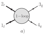
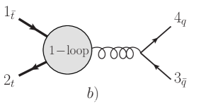
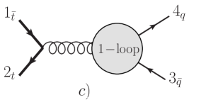
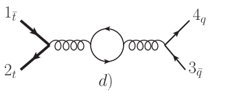
In Ref. [16], numerical results for spin-averaged squared amplitudes for the virtual corrections were given for a particular kinematic point. In Appendix B, we give numerical results for most of the helicity amplitudes for that kinematic point. We have checked the calculation in several ways. For example, our primitive amplitudes have correct $1/\epsilon$ poles [51] and are gauge invariant, once mass counter-terms are accounted for. We performed a diagrammatic check comparing amplitudes computed through unitarity and on-shell matrix elements with a similar, but independent, implementation of the OPP procedure [35] which is applicable to individual Feynman diagrams. Finally, we have checked that when we compute the spin-averaged amplitude squared for the kinematic point considered in Ref. [16], we find full agreement with their results.

A well-known problem that occurs in the process of the reduction of one-loop diagrams to any basis of scalar integrals is the appearance of unphysical singularities at the intermediate stages of the calculation. Those singularities cancel in the final result as a matter of principle but it has been proven to be difficult to achieve such cancellations in practice if reductions are performed numerically. Within the current calculation, we control potential numerical instabilities by requiring that the $1/\epsilon$ pole of a primitive amplitudes is calculated correctly to within ${\cal O}(10^{-4})$. If this condition is not fulfilled, the program switches from double to quadruple precision and re-calculates the offending amplitude. The number of points that needs to be re-calculated is typically small, below a percent for partonic channels that we consider.

3.3 Real emission processes and soft-collinear subtraction counter-terms

Computation of the real emission corrections and subtraction counter-terms is an important part of any NLO computation. There are three generic processes that need to be considered: $0\to\bar{t}t+gggg$, $0\to\bar{t}t+\bar{q}q+gg$ and $0\to\bar{t}t+\bar{q}q+\bar{q}^{\prime}q^{\prime}$. Once amplitudes for those processes are known, all partonic channels that contribute to the real emission correction to the hadronic production of $t\bar{t}+{\rm jet}$ can be constructed. We employ color decomposition to express those amplitudes through color-ordered ones and use Berends-Giele recurrence relations [52] to compute the latter. Below results for color decomposition of the relevant tree amplitudes are summarized.

The color decomposition for the amplitude $0\to\bar{t}t+gggg$ has already been given in Eq.(33). The color decomposition for the amplitude $0\to\bar{t}t+\bar{q}q+gg$ in double index notation for the gluon field reads [53]

$${\cal A}(\bar{t},t,\bar{q},q,g_{1},g_{2})=g_{s}^{4}\sum\limits_{\sigma\in S_{2}}\Bigg{(}\delta^{i_{t}}_{j_{\bar{q}}}\delta^{i_{q}}_{j_{\sigma(1)}}\delta^{i_{\sigma(1)}}_{j_{\sigma(2)}}\delta^{i_{\sigma(2)}}_{j_{\bar{t}}}A(\bar{t},t,{\bar{q}},q,g_{\sigma(1)},g_{\sigma(2)})$$

$$+\delta^{i_{t}}_{j_{\sigma(1)}}\delta^{i_{\sigma(1)}}_{j_{\sigma(2)}}\delta^{i_{\sigma(2)}}_{j_{\bar{q}}}\delta^{i_{q}}_{j_{\bar{t}}}A(\bar{t},t,g_{\sigma(1)},g_{\sigma(2)},{\bar{q}},q)+\delta^{i_{t}}_{j_{\sigma(1)}}\delta^{i_{\sigma(1)}}_{j_{\bar{q}}}\delta^{i_{q}}_{j_{\sigma(2)}}\delta^{i_{\sigma(2)}}_{j_{\bar{t}}}A(\bar{t},t,g_{\sigma(1)},{\bar{q}},q,g_{\sigma(2)})$$

$$-\frac{1}{N_{c}}\delta^{i_{t}}_{j_{\sigma(2)}}\delta^{i_{\sigma(2)}}_{j_{\sigma(1)}}\delta^{i_{\sigma(1)}}_{j_{\bar{t}}}\delta^{i_{q}}_{j_{\bar{q}}}A(\bar{t},g_{\sigma(1)},g_{\sigma(2)},t,\bar{q},q)-\frac{1}{N_{c}}\delta^{i_{t}}_{j_{\sigma(1)}}\delta^{i_{\sigma(1)}}_{j_{\bar{t}}}\delta^{i_{q}}_{j_{\sigma(2)}}\delta^{i_{\sigma(2)}}_{j_{\bar{q}}}A(\bar{t},g_{\sigma(1)},t,\bar{q},g_{\sigma(2)},q)$$

$$-\frac{1}{N_{c}}\delta^{i_{q}}_{j_{\sigma(2)}}\delta^{i_{\sigma(2)}}_{j_{\sigma(1)}}\delta^{i_{\sigma(1)}}_{j_{\bar{q}}}\delta^{i_{t}}_{j_{\bar{t}}}A(\bar{t},t,\bar{q},g_{\sigma(1)},g_{\sigma(2)},q)\Bigg{)}.$$

Finally, the color decomposition for the six quark amplitude for non-identical quarks $0\to\bar{t}t+\bar{q}q+\bar{f}f$ reads

$${\cal A}(\bar{t},t,\bar{q},q,\bar{f},f) = \delta^{i_{t}}_{j_{\bar{q}}}\delta^{i_{q}}_{j_{\bar{f}}}\delta^{i_{f}}_{j_{\bar{t}}}A(\bar{t},t,\bar{q},q,\bar{f},f)+\delta^{i_{t}}_{j_{\bar{f}}}\delta^{i_{f}}_{j_{\bar{q}}}\delta^{i_{q}}_{j_{\bar{t}}}A(\bar{t},t,\bar{f},f,\bar{q},q)$$ (40)

$$-\frac{1}{N_{c}}\left(\delta^{i_{q}}_{j_{\bar{q}}}\delta^{i_{t}}_{j_{\bar{f}}}\delta^{i_{f}}_{j_{\bar{t}}}+\delta^{i_{t}}_{j_{\bar{t}}}\delta^{i_{f}}_{j_{\bar{q}}}\delta^{i_{q}}_{j_{\bar{f}}}-\frac{1}{N_{c}}\delta^{i_{t}}_{j_{\bar{t}}}\delta^{i_{f}}_{j_{\bar{f}}}\delta^{i_{q}}_{j_{\bar{q}}}\right)A(\bar{t},f,\bar{q},q,\bar{f},t)$$

$$-\frac{1}{N_{c}}\left(\delta^{i_{f}}_{j_{\bar{f}}}\delta^{i_{t}}_{j_{\bar{q}}}\delta^{i_{q}}_{j_{\bar{t}}}+\delta^{i_{q}}_{j_{\bar{q}}}\delta^{i_{f}}_{j_{\bar{t}}}\delta^{i_{t}}_{j_{\bar{f}}}-\frac{1}{N_{c}}\delta^{i_{t}}_{j_{\bar{t}}}\delta^{i_{f}}_{j_{\bar{f}}}\delta^{i_{q}}_{j_{\bar{q}}}\right)A(\bar{t},f,\bar{f},t,\bar{q},q)$$

$$-\frac{1}{N_{c}}\left(\delta^{i_{f}}_{j_{\bar{f}}}\delta^{i_{t}}_{j_{\bar{q}}}\delta^{i_{q}}_{j_{\bar{t}}}+\delta^{i_{t}}_{j_{\bar{t}}}\delta^{i_{f}}_{j_{\bar{q}}}\delta^{i_{q}}_{j_{\bar{f}}}-\frac{1}{N_{c}}\delta^{i_{t}}_{j_{\bar{t}}}\delta^{i_{f}}_{j_{\bar{f}}}\delta^{i_{q}}_{j_{\bar{q}}}\right)A(\bar{t},q,\bar{f},f,\bar{q},t).$$

The amplitude for the identical quarks ${\cal A}(\bar{t},t,\bar{q},q,\bar{q},q)$ can be obtained from the previous amplitude by the anti-symmetrization procedure

$${\cal A}(\bar{t},t,\bar{q},q,\bar{q},q)={\cal A}(\bar{t},t,\bar{q},q,\bar{f},f)-{\cal A}(\bar{t},t,\bar{q},f,\bar{f},q).$$ (41)

We note that many of the amplitudes required for the computation of the real emission corrections are also employed for the computation of the virtual corrections within the unitarity framework. We use one and the same program that computes the on-shell tree amplitudes for complex or real external momenta, as needed for the virtual and the real corrections, respectively. We checked our calculation of the real emission matrix elements against Madgraph [54] for all the partonic channels.

As it is typical for NLO calculations, when we integrate the real emission matrix elements with $t\bar{t}$ and two additional partons in the final state over the phase-space constrained by the requirement that a $t\bar{t}$ pair and at least one jet is observed, we encounter infra-red and collinear divergences. Those divergences are removed by the subtraction procedure. We use dipole formalism of Ref. [55] extended to deal with the QCD radiation off massive particles in Ref. [56]. We note that in the original publications, the subtraction terms were integrated over full unresolved phase-space which is not very convenient. An optimization of the subtraction procedure, where subtractions are only performed if the event kinematics is close to singular, was suggested in Ref. [57]. Dipoles integrated over the restricted phase-space including the case of massive emitters and spectators can be found in Ref. [23, 58, 59, 60]. In the actual implementation of the subtraction procedure, we closely follow Ref. [58]. We have checked that our results do not depend on the parameter that restrict the integration over the dipole phase-space; this is a useful way to check the consistency of the implementation of the subtraction terms.

Figure 2: Top quark transverse momentum (a) and rapidity (b) distributions (MS) computed through NLO QCD for $pp\to t\bar{t}j$, at the LHC ($\sqrt{s}=14~{}{\rm TeV}$) compared to the results of Refs. [15, 16] (DUW). The renormalization and factorization scales are set to $\mu=m_{t}$.

4 Results

In this Section we present the results of the calculation of the NLO QCD corrections to $t\bar{t}$ pair production in association with one hard jet at the Tevatron and the LHC. We begin by comparing our results with that of Refs. [15, 16]. Then we present the results that include the top quark decays.

4.1 Input parameters and comparison with existing results

For the comparison with Refs. [15, 16], we need to choose identical input parameters. To this end, we use the top quark mass $m_{t}=174~{}{\rm GeV}$. Also, the parton distribution functions CTEQ6L1/6M have been updated since the results of Ref. [15, 16] appeared; therefore, for the comparison we employ their older versions. Finally, the $k_{\perp}$-clustering algorithm with $R_{ij}=\sqrt{(y_{i}-y_{j})^{2}-(\phi_{i}-\phi_{j})^{2}}=1$ and $E_{\perp}$-weighted recombination scheme [61] is used to define jets in Refs. [15, 16]. The jet transverse momentum cut $p_{\perp,j}=50(20)~{}{\rm GeV}$ is employed for the LHC (Tevatron), respectively. When we use those parameters in the calculation, we obtain good agreement with Refs. [15, 16]. We quote our results for the LHC ($\sqrt{s}=14~{}{\rm TeV}$), with the factorization and the renormalization scales set to $m_{t}$. For the total cross-section we obtain

$$\sigma^{\rm NLO}(pp\to t\bar{t}j)=375.8(1.0)~{}{\rm pb},$$ (42)

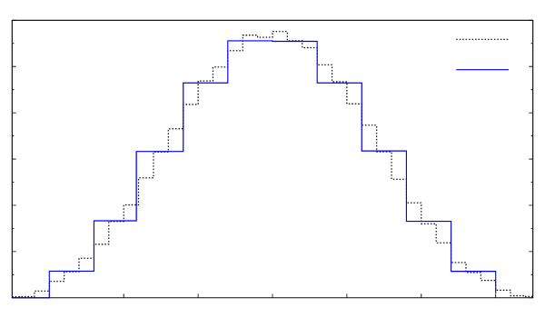
which agrees well with the result $376.2~{}{\rm pb}$ quoted in Refs. [15, 16]. We note that the NLO QCD $pp\to t\bar{t}j$ cross-section at the LHC for the input parameters of Refs. [15, 16] was also reported in Ref. [17] where the result $376.6~{}{\rm pb}$ was found. We have checked that similar level of agreement – one percent or better – persists for cross-sections evaluated for other values of the renormalization and factorization scales, for both the Tevatron and the LHC. We have also verified that we reproduce kinematic distributions presented in Refs. [15, 16]. As an illustration, our results for the transverse momentum and the rapidity distributions of the top quarks at the LHC, computed through NLO QCD, are compared with similar distributions from Refs. [15, 16] in Fig. 2. Good agreement between the two results is apparent. We also confirm an observation in Refs. [15, 16] that the forward-backward asymmetry of top quarks in $t\bar{t}+{\rm jet}$ production at the Tevatron is significantly reduced if NLO QCD effects are taken into account. For $\mu=m_{t}$ and the jet transverse momentum cut of $20~{}{\rm GeV}$, we find the forward-backward asymmetry computed through NLO QCD to be $-2.28\%$, in agreement with $-2.27\%$ reported in Refs. [15, 16]. We discuss the forward-backward asymmetry in more detail below, when we report on our calculation that includes decays of top quarks.

Figure 3: Various distributions for the process $p\bar{p}\to(t\to l^{+}\nu b)+(\bar{t}\to j_{1}j_{2}\bar{b})+j$ at the Tevatron at leading (blue) and next-to-leading order (red) in perturbative QCD. The bands correspond to the choice of the renormalization and factorization scales $\mu=[m_{t}/2,m_{t},2m_{t}]$. We show distributions of the transverse momentum (a) and rapidity of the positron (b), the total transverse energy $H_{\perp}$ (c), the transverse momentum (d) and the rapidity (e) distributions of the fifth hardest jet and the missing transverse momentum (f).

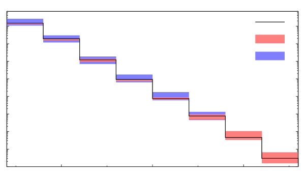
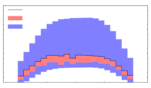
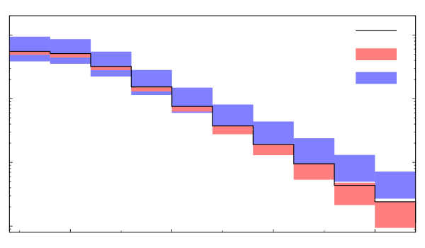
Having performed an extensive comparison with results of Refs. [15, 16], we turn to the discussion of observables that can be studied if decays of top quarks are accounted for in the calculation. We consider two primary scenarios – $t\bar{t}j$ as the signal process and as the background process to weak boson fusion production of the Higgs boson. It is important to consider these different scenarios because we want to understand to what extent applied cuts affect the radiative corrections. We begin with the discussion of the $pp(p\bar{p})\to t\bar{t}j$ production in the kinematic region which is usually employed to study top quarks. We perform separate studies for the Tevatron and the LHC. We choose two center of mass energies $\sqrt{s}=7~{}{\rm TeV}$ and $\sqrt{s}=14~{}{\rm TeV}$ for the LHC and one center of mass energy $\sqrt{s}=1.96~{}{\rm TeV}$ for the Tevatron. We use the following values for the top quark and the $W$-boson masses $m_{t}=172~{}{\rm GeV}$, $m_{W}=80.419~{}{\rm GeV}$ and employ CTEQ6L1 and CTEQ6.1M parton distribution functions in LO and NLO calculations, respectively. We employ the $k_{\perp}$ jet algorithm with $R_{ij}=0.5$ and the four-momentum recombination scheme. The couplings of the $W$-boson to fermions are obtained from the Fermi constant $G_{\mathrm{F}}=1.16639\cdot 10^{-5}\,{\rm GeV}^{-2}$. We emphasize that results reported in this paper are calculated with on-shell top quark decays at leading order in QCD; radiative corrections to the decays are not included. We take the CKM matrix to be the identity matrix. We consider the $W$-boson in $t\to Wb$ decay to be on the mass shell. With these approximations, we obtain the leading order top quark decay width $\Gamma_{t}=1.47~{}{\rm GeV}$. We set the width of the $W$ boson to $2.14~{}{\rm GeV}$. With our input parameters, we find the following branching ratios ${\rm Br}(W^{+}\to l^{+}\nu)=10.6~{}\%$, ${\rm Br}(W^{+}\to{\rm hadrons})=64~{}\%$. We note that the hadronic branching fraction is slightly lower than the experimental value $67~{}\%$.

4.2 $t\bar{t}+{\rm jet}$ production in lepton + jets channel at the Tevatron

We begin our discussion with the Tevatron, $\sqrt{s}=1.96~{}{\rm TeV}$. The measurement of the $p\bar{p}\to t\bar{t}+{\rm jet}$ at the Tevatron was performed by the CDF collaboration and there is a public note [63] that describes the details of the experimental setup and the results of the measurements. For our purposes, we can take all the selection criteria for $p\bar{p}\to t\bar{t}j$ from that reference. We consider events where top quark decays leptonically and the anti-top quark decays hadronically. We require that there are five or more jets in the event and that two of these jets are $b$-jets. It is to be understood that a $b$-jet is defined as a jet that originates from the $tWb$ vertex. For $p\bar{p}\to t\bar{t}j$ process, this leads to a misidentification of $b$-jets, that originate from $t\bar{t}$ production, as non-$b$ jets. However, this is a minor issue since $b$-jets in the production process appear infrequently. The lepton transverse momentum and the missing energy in the event should satisfy $p_{\perp,l}>20~{}{\rm GeV}$, $E_{\perp}^{\rm miss}>20~{}{\rm GeV}$. The jet transverse momenta are required to be larger than $p_{\perp,j}>20~{}{\rm GeV}$ and jets must be central $|y_{j}|<2$. There is an additional cut on the transverse energy in the event $H_{\perp}=\sum_{j}p_{\perp,j}+p_{\perp,e}+E_{\perp}^{\rm miss}$, needed to better discriminate against the background. It is required that $H_{\perp}>220~{}{\rm GeV}$.

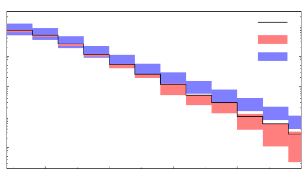
We first present the results for total cross-sections. We set the renormalization and factorization scales equal to each other and consider three values $\mu=[m_{t}/2,m_{t},2m_{t}]$. We obtain

$$\sigma_{\rm LO}(p\bar{p}\to(t\to l^{+}\nu b)\;+(\bar{t}\to j_{1}j_{2}\bar{b})+j)=36.9^{+22.1}_{-12.8}~{}{\rm fb};$$

$$\sigma_{\rm NLO}(p\bar{p}\to(t\to l^{+}\nu b)\;+(\bar{t}\to j_{1}j_{2}\bar{b})+j)=33.6^{-4.0}_{-3.6}~{}{\rm fb},$$ (43)

where the central value refers to $\mu=m_{t}$, the upper value to $\mu=m_{t}/2$ and the lower value to $\mu=2m_{t}$. The improvement in the scale stability at next-to-leading order is apparent.

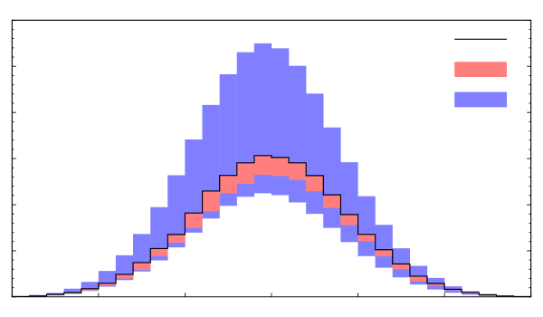
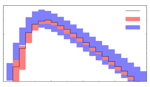
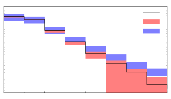
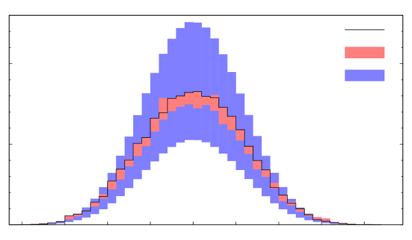
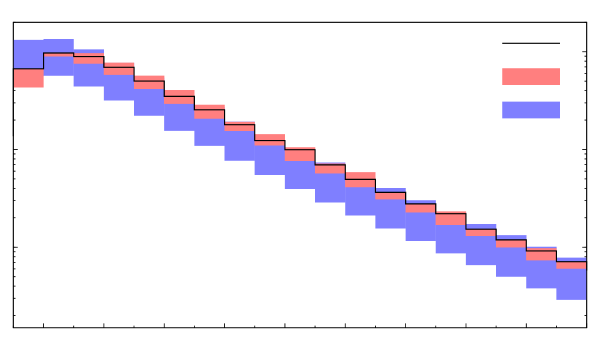
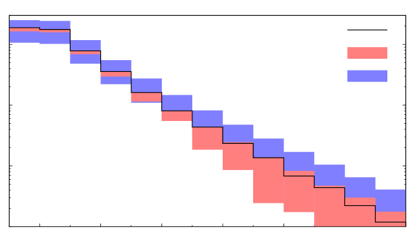
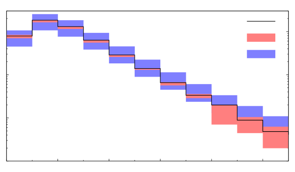
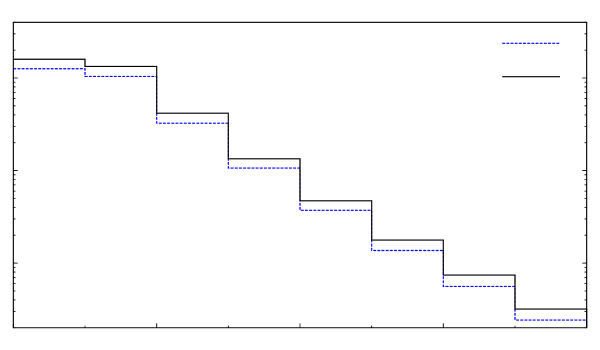
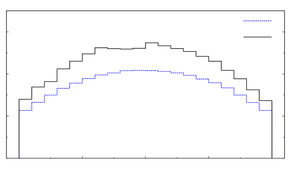
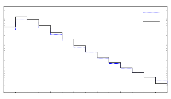
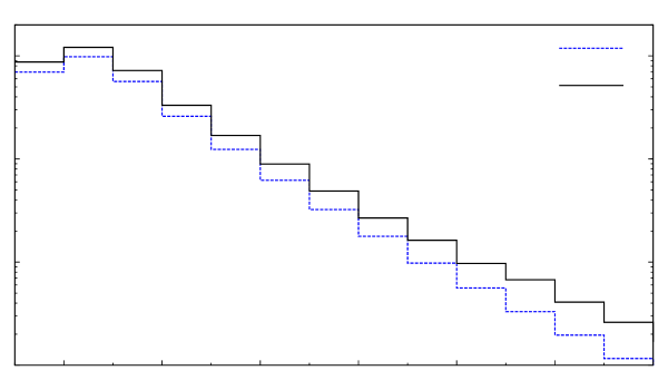
Our results for the kinematic distributions of the transverse momentum and the rapidity of the charged lepton $l^{+}$, the total transverse energy $H_{\perp}$, the transverse momentum and the rapidity of the fifth hardest jet and the missing transverse energy are shown in Fig. 3(a)-(f), respectively. The bands correspond to choices of the renormalization and factorization scales $\mu=[m_{t}/2,m_{t},2m_{t}]$. We observe that the scale variation in rapidity distributions is in line with the total cross-section modification and there is little change in shape. However, for the transverse momenta distributions and the $H_{\perp}$ distribution, the situation is more subtle. There are clear differences in shapes between distributions computed at leading and next-to-leading order and, in addition, there are kinematic regions where the scale variation bands at LO and NLO do not overlap. In particular, this happens at the high end of the lepton transverse momentum distribution where, in addition, the scale variation at NLO actually exceeds the scale variation at leading order. Similar phenomenon occurs in the missing transverse energy distribution. On the contrary, the scale variation of the transverse momentum distribution of the fifth hardest jet is modest at high $p_{\perp,j}$.

It is interesting that some of the distributions exhibit peculiar shape distortions. We stress that these distortions depend in a very significant way on the choice of the renormalization and factorizations scales in leading order computations and that it is entirely possible that some of the changes that we observe in Fig. 3 can be accommodated by a kinematic-dependent choice of the renormalization scale. We will not pursue this topic further in the current paper; for a related discussion in the context of $W+{\rm jets}$ production, see Refs. [64, 65, 66, 67]. For our choices of scales, we observe that the charged lepton transverse momentum distribution and the missing transverse energy distribution become softer at NLO when compared to corresponding leading order distributions. We can understand this by observing that for $\mu=m_{t}$, the transverse momentum distribution of the top quarks becomes softer at NLO as well [15, 16]. On the other hand, $\mu=m_{t}$ is almost the perfect choice of the renormalization scale for the transverse momentum distribution of the fifth hardest jet; this is probably just a numerical coincidence. While $H_{\perp}$ distribution does not show significant distortion at high $H_{\perp}$, the (broad) peak of the $H_{\perp}$ distribution shifts to higher $H_{\perp}$ values and there is a depletion at low $H_{\perp}$ values.

Finally, it is clear from Fig. 3 that the positron rapidity distribution becomes much more symmetric at next-to-leading order. To quantify this, we compute the positron forward-backward asymmetry

$$A_{e^{+}}=\frac{\sigma(y_{e^{+}}>0)-\sigma(y_{e^{+}}<0)}{\sigma(y_{e^{+}}>0)+\sigma(y_{e^{+}}<0)},\;\;\;y_{e^{+}}=\frac{1}{2}\ln\left(\frac{E{{}_{e^{+}}}+p_{z,e^{+}}}{E_{e^{+}}-p_{z,e^{+}}}\right).$$ (44)

For the set up described above, we find the positron asymmetry to be strongly reduced at next-to-leading order, similar to the top quark asymmetry [15, 16]. We obtain

$$A_{e^{+}}^{\rm LO}=-5.05~{}\%,~{}~{}~{}~{}~{}~{}~{}A_{e^{+}}^{\rm NLO}=-0.5~{}\%.$$ (45)

At first sight, the strong reduction in the positron forward-backward asymmetry observed in $p\bar{p}\to t\bar{t}j$ process at NLO is rather puzzling and worrisome since it suggests a breakdown of the perturbative expansion for this quantity. We will now argue that i) these worries are unfounded; ii) the large reduction in the forward-backward asymmetry in $p\bar{p}\to t\bar{t}j$ at NLO is natural; and iii) the NLO asymmetry is, most likely, stable against yet higher order corrections. To build up the argument, we consider the limit of the low jet transverse momentum cut $p_{\perp j}\to 0$.

We notice that, by requiring additional jet in the final state and by taking $p_{\perp j}$ to be small, we introduce two types of degrees of freedom: soft degrees of freedom, controlled by the jet transverse momentum cut $p_{\perp j}$ and hard degrees of freedom, controlled by the mass of the top quark. The crux of our argument is that the asymmetry in $t\bar{t}j$ can be generated by both soft and hard degrees of freedom but those mechanisms appear at two consecutive orders in perturbation theory. The “soft” asymmetry appears at leading order while the “hard” asymmetry appears at next-to-leading order. As evident from their very different dependence on $p_{\perp,j}$, these two mechanisms are unrelated. Hence, the dramatic change in the asymmetry at next-to-leading order should not be taken as an indicator that the perturbative expansion for this observable breaks down.

We now explain this argument in detail. We discuss the top quark asymmetry rather than the positron asymmetry, for simplicity. In the limit of small $p_{\perp j}$, the leading order asymmetry is generated when the soft gluon between initial ($q\bar{q}$) and final ($t\bar{t}$) states is exchanged. Since the interference diagrams are non-singular in the collinear limit, the difference of the forward and backward cross-sections at leading order can only be proportional to a single logarithm of the infra-red cut-off

$$[\sigma(y_{t}>0)-\sigma(y_{t}<0)]_{\rm LO}\approx\sigma_{A}\ln\left(\frac{m_{t}}{p_{\perp,j}}\right),\;\;\ y_{t}=\frac{1}{2}\ln\left(\frac{E_{t}+p_{t,z}}{E_{t}-p_{t,z}}\right).$$ (46)

Here, $\sigma_{A}$ is some quantity with the dimension of the cross-section and $y_{t}$ is the top quark rapidity. On the other hand, the total cross-section that appears in the denominator in the definition of the asymmetry Eq.(44) depends on the double logarithm of the jet transverse momentum cut

$$\sigma(y_{t}>0)+\sigma(y_{t}<0)\sim\frac{2C_{\mathrm{F}}\alpha_{s}}{\pi}\ln^{2}\left(\frac{m_{t}}{p_{\perp,j}}\right)\;\sigma_{t\bar{t}}.$$ (47)

In Eq.(47), $\sigma_{t\bar{t}}$ is the production cross-section for $p\bar{p}\to t\bar{t}$. As the result

$$A_{t\bar{t}j}^{\rm LO}(p_{\perp,j})=\frac{\sigma(y_{t}>0)-\sigma(y_{t}<0)}{\sigma(y_{t}>0)+\sigma(y_{t}<0)}\sim\ln^{-1}\left(\frac{m_{t}}{p_{\perp,j}}\right).$$ (48)

Hence, we see that at leading order in perturbative QCD, the asymmetry in $p\bar{p}\to t\bar{t}j$ is generated by soft degrees of freedom and that this asymmetry decreases with the decrease in the jet transverse momentum cut $p_{\perp,j}$.

Figure 4: Various distributions for the process $pp\to(t\rightarrow l^{+}\nu b)+(\bar{t}\rightarrow l^{-}\bar{\nu}\bar{b})+j$ at the LHC ($\sqrt{s}=7~{}{\rm TeV}$) at leading (blue) and next-to-leading order (red) in perturbative QCD. The bands correspond to the choice of the renormalization and factorization scales $\mu=[m_{t}/2,m_{t},2m_{t}]$. We show distributions of the transverse momentum (a) and rapidity (b) of the positron, the total transverse energy $H_{\perp}$ (c), the transverse momentum distribution of the third hardest jet (d) and the invariant mass of the two leptons (e).

At next-to-leading order, the asymmetry can still be generated by soft exchanges. In such a case, it is natural to expect that moderate correction to the leading order asymmetry Eq.(48) is generated. However, it is interesting that at next-to-leading order, a new mechanism for generating the asymmetry in $p\bar{p}\to t\bar{t}j$ appears. Indeed, we can use hard degrees of freedom to generate the asymmetry, in much the same way as it is generated in the inclusive $p\bar{p}\to t\bar{t}$ process. In addition, we can use the emission of an additional soft and collinear jet from the initial state to provide conventional double logarithmic enhancement of this “hard” asymmetry. This mechanism leads to the following forward-backward cross-section difference in Eq.(44) as

$$\sigma(y_{t}>0)-\sigma(y_{t}<0)\sim\frac{2C_{\mathrm{F}}\alpha_{s}}{\pi}\ln^{2}\left(\frac{m_{t}}{p_{\perp,j}}\right)\;A_{t\bar{t}}\;\sigma_{t\bar{t}},$$ (49)

where $A_{t\bar{t}}$ is the $p\bar{p}\to t\bar{t}$ inclusive asymmetry. Taking the ratio of Eq.(49) and Eq.(47), we find

$$A_{t\bar{t}j}^{\rm hard}\approx A_{t\bar{t}}.$$ (50)

The full forward-backward asymmetry at next-to-leading order is given by the sum of the two mechanisms

$$A_{t\bar{t}j}^{\rm NLO}\approx A_{t\bar{t}j}^{\rm soft}(p_{\perp,j})+A_{t\bar{t}j}^{\rm hard}.$$ (51)

Following the preceding discussion, we estimate

$$A_{t\bar{t}j}^{\rm soft}(p_{\perp,j})\sim A_{t\bar{t}j}^{\rm LO}(p_{\perp,j})\sim\ln^{-1}\left(\frac{m_{t}}{p_{\perp,j}}\right),\;\;\;A_{t\bar{t}j}^{\rm hard}\approx A_{t\bar{t}}.$$ (52)

Numerically, the “soft” asymmetry at $p_{\perp,j}=30~{}{\rm GeV}$ is $A_{t\bar{t}j}^{\rm LO}(30~{}{\rm GeV})\sim-7\%$ and the “hard” asymmetry is $A_{t\bar{t}}\sim 5\%$ [68], so that the significant reduction in the leading order $p\bar{p}\to t\bar{t}j$ asymmetry is observed, once the NLO QCD corrections are accounted for. A peculiar consequence of this argument is that, in the limit of a very small jet transverse momentum cut, the top quark forward-backward asymmetries in the $p\bar{p}\to t\bar{t}j$ process and in the inclusive $p\bar{p}\to t\bar{t}$ process coincide

$$\lim_{p_{\perp,j}\to 0}A_{t\bar{t}j}(p_{\perp,j})\to A_{t\bar{t}},$$ (53)

because the “soft” component of the asymmetry vanishes as the inverse logarithm of the cut on the jet transverse momentum.

We stress that the observation by Dittmaier, Uwer and Weinzierl of the large NLO QCD corrections to the top quark forward-backward asymmetry in $p\bar{p}\to t\bar{t}j$ [15, 16] is important outside the context of that computation. Indeed, since the asymmetry in $p\bar{p}\to t\bar{t}$ appears at NLO and since NLO is the highest order in the perturbative expansion available for that process, corrections to the inclusive asymmetry are not known. On the other hand, because the asymmetry in $p\bar{p}\to t\bar{t}j$ appears already at leading order, a NLO QCD computation for $p\bar{p}\to t\bar{t}j$ gives corrections to the leading order forward-backward asymmetry. The fact that these corrections turn out to be nearly $100\%$, as discovered in Refs. [15, 16], leads to doubts about the robustness of the existing predictions for the inclusive asymmetry in the $p\bar{p}\to t\bar{t}$ process. Of course, the issue of robustness is rather important given the existing discrepancy between the measurement of the asymmetry in $p\bar{p}\to t\bar{t}$ [8, 9] and the theoretical prediction [68].

We believe that our argument supports the robustness of the theoretical prediction of the inclusive asymmetry $A_{t\bar{t}}$. In fact, as we have explained, there are two physically distinct mechanisms that generate the asymmetry in $p\bar{p}\to t\bar{t}j$. These mechanisms are related to the existence of two types of degrees of freedom, which can be clearly separated by lowering the cut on the jet transverse momentum. The only peculiarity about the asymmetry is that the two mechanisms for the asymmetry generation do not appear at the same order of the perturbative expansion which leads to apparent problems with the interpretation of its convergence. Needless to say that we do not see any other mechanism that can start contributing to the asymmetry at next-to-next-to-leading order (NNLO) and beyond. Therefore, we believe, that the NLO prediction for the asymmetry in $p\bar{p}\to t\bar{t}j$ is robust. Similarly, since inclusive $p\bar{p}\to t\bar{t}$ production process is only sensitive to hard degrees of freedom, no new mechanism for the asymmetry generation can appear at NNLO and beyond. Therefore, we believe that the existing prediction for the top quark forward-backward asymmetry in $p\bar{p}\to t\bar{t}$ is robust as well.

Figure 5: Kinematic distributions for the process $pp\to(t\to l^{+}\nu b)+(\bar{t}\to l^{-}\bar{\nu}\bar{b})+j$ at the LHC ($\sqrt{s}=14~{}{\rm TeV}$) with weak boson fusion cuts. The renormalization and factorization scales are set to $\mu=m_{t}$. Distributions at leading (blue) and next-to-leading (black) order in perturbative QCD are shown. We show distributions of the transverse momentum (a) and rapidity of the electron (b), the invariant mass of the electron and the positron (c), the transverse momentum of the leading jet (d).

4.3 $t\bar{t}+{\rm jet}$ production in dilepton channel at the LHC

We now turn our attention to the LHC, $\sqrt{s}=7~{}{\rm TeV}$. We consider dilepton channel and require three or more jets with $p_{\perp,j}>50~{}{\rm GeV}$, $p_{\perp,\mathrm{b-jet}}>20~{}{\rm GeV}$. Our definition of the $b$-jet is explained above. We also apply the following cuts on the lepton transverse momentum $p_{\perp,l}>20~{}{\rm GeV}$ and the missing transverse momentum $p_{\perp,\rm miss}>40~{}{\rm GeV}$. We begin by showing the cross-sections for the three values of the factorization and renormalization scales $\mu=[m_{t}/2,m_{t},2m_{t}]$. We find

$$\sigma_{\rm LO}(pp\to(t\to l^{+}\nu b)\;+(\bar{t}\to l^{-}\bar{\nu}\bar{b})+j)=229.9^{+133.7}_{-78.2}~{}{\rm fb};$$

$$\sigma_{\rm NLO}(pp\to(t\to l^{+}\nu b)\;+(\bar{t}\to l^{-}\bar{\nu}\bar{b})+j)=256.5^{-14.8}_{-25.6}~{}{\rm fb},$$ (54)

where the central value refers to $\mu=m_{t}$, the upper value to $\mu=m_{t}/2$ and the lower value to $\mu=2m_{t}$. Similar to the Tevatron case, the NLO cross-section is very stable against changes in the renormalization and factorization scales, in contrast to the leading order result.

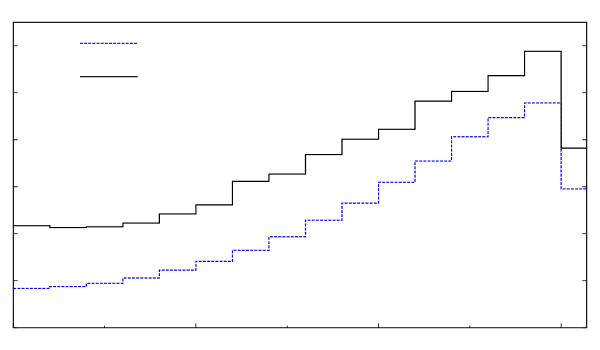
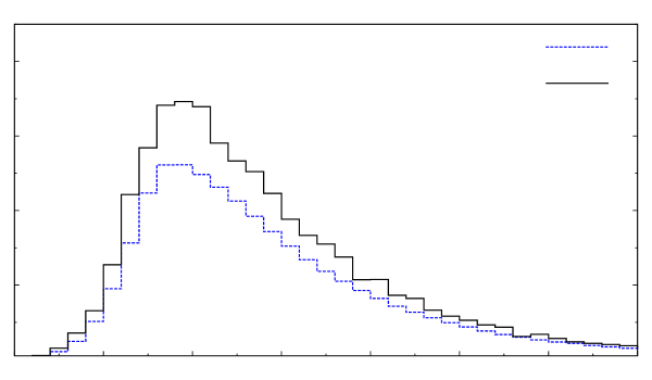
Our results for kinematic distributions are displayed in Fig. 4, where we present the transverse momentum and the rapidity distributions of the positively charged lepton, the distribution of the total transverse energy $H_{\perp}$, the transverse momentum distribution of the third hardest jet and the distribution of the invariant mass of the two leptons. We note that for some choices of the renormalization and factorization scales, the NLO results for the lepton transverse momentum distribution become negative at high $p_{\perp}(l^{+})\mbox{\raisebox{-1.29167pt}{\footnotesize$\>\stackrel{{\scriptstyle>}}{{\sim}}\>$}}400~{}{\rm GeV}$. This indicates that $\mu=m_{t}/2$ is too low a scale for this observable and that there is large residual scale dependence in this observable even at next-to-leading order. The $H_{\perp}$-distribution is shifted to higher values, leading to positive corrections in the high-$H_{\perp}$ tail. The transverse momentum distribution of the third jet becomes softer and the lepton invariant mass distribution is only marginally affected. Many of these features can probably be understood by performing a leading order computation with the kinematic-dependent choices of the scales. As we already mentioned in the context of the Tevatron discussion, we do not pursue this topic in the present paper and reserve it for future work.

Figure 6: Kinematic distributions for the process $pp\to(t\to l^{+}\nu b)+(\bar{t}\to l^{-}\bar{\nu}\bar{b})+j$ at the LHC ($\sqrt{s}=14~{}{\rm TeV}$) with weak boson fusion cuts. The renormalization and factorization scales are set to $\mu=m_{t}$. Distributions at leading (blue) and next-to-leading (black) order in perturbative QCD are shown. We show distributions relevant for the discrimination between the signal and the background. In particular, we display distributions of the relative azimuthal angle of the electron and the positron (a), the $m_{T}$ variable (b) (see text), the rapidity of the leading jet (c), the rapidity of the second leading jet (d) and the relative rapidity of the “veto” (third hardest) jet (e). For the definition of the relative rapidity of the veto jet, see text.

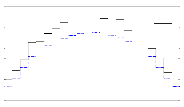
Our last example concerns NLO QCD corrections to $pp\to t\bar{t}j$ process in the kinematic region relevant for the Higgs boson searches in weak boson fusion $pp\to jjH\to jjW^{+}W^{-}$ production channel, with leptonic decays of the $W$-bosons. It was shown in Ref. [69] that the $pp\to t\bar{t}j$ process is the largest background to the weak boson fusion signal. For our calculation, we take the LHC energy to be $\sqrt{s}=14~{}{\rm TeV}$. The event selection is based on the following cuts [69]. We define jets with the usual $k_{\perp}$ algorithm, $R_{ij}=0.5$ and the transverse momentum cut $p_{\perp,j}>20~{}{\rm GeV}$. The two jets with the highest transverse momentum (tag jets) are required to satisfy $p_{\perp}^{(1)}>40~{}{\rm GeV}$ and $p_{\perp}^{(2)}>20~{}{\rm GeV}$. Those jets should be in the opposite hemispheres $y_{1}y_{2}<0$ and widely separated in rapidity $|y_{1}-y_{2}|>3.0$. The invariant mass of the two tag jets should be large $m_{j_{1}j_{2}}>550~{}{\rm GeV}$. The two leptons are required to have large transverse momenta $p_{\perp,l}>20~{}{\rm GeV}$ and central rapidities $|y_{l}|<2$. In principle, there are other cuts that are imposed to separate the weak boson fusion signal but we do not employ those cuts in what follows. For the cross-sections at $\mu=m_{t}$ we find

$$\sigma_{\rm LO}(pp\to(t\to l^{+}\nu b)\;+(\bar{t}\to l^{-}\bar{\nu}\bar{b})+j)=139.6~{}{\rm fb};$$

$$\sigma_{\rm NLO}(pp\to(t\to l^{+}\nu b)\;+(\bar{t}\to l^{-}\bar{\nu}\bar{b})+j)=177.9~{}{\rm fb}.$$ (55)

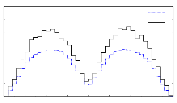
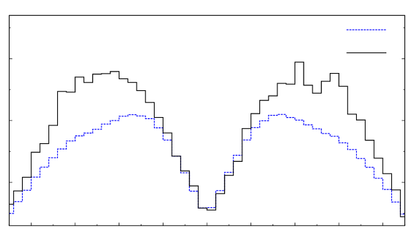
The next-to-leading order cross-section exceeds the leading order cross-section by twenty-five percent which is not unusual. In Fig. 5 we show a number of kinematic distributions for the weak boson fusion cuts. In particular, lepton transverse momentum and rapidity distributions, distribution of the dilepton invariant mass and the transverse momentum distribution of the hardest jet are displayed. In Fig. 6, we show kinematic distributions that can be used to discriminate between the $t\bar{t}+{\rm jet}$ background and the weak boson fusion signal. We display the distribution in the relative azimuthal angle of the two leptons, the distribution of the approximate transverse mass of the two $W$-bosons $m_{T}$ and some rapidity distributions. The definition of the $m_{T}$-variable is given in Ref. [69]

$$m_{T}=\left[\left(E_{\perp,l^{+}l^{-}}+{\tilde{E}}_{\perp,{\rm miss}}\right)^{2}-\left({\mbox{\boldmath$p$}}_{\perp,l^{+}l^{-}}+{\mbox{\boldmath$p$}}_{\perp,{\rm miss}}\right)^{2}\right]^{1/2}.$$ (56)

In this formula, $p_{\perp,{\rm miss}}$ is the missing transverse momentum which we associate with the vector sum of the momenta of the two neutrinos and ${\tilde{E}}_{\perp,\rm miss}=\sqrt{p_{\perp,{\rm miss}}^{2}+m_{l^{+}l^{-}}^{2}}$. As explained in Ref. [69], $m_{T}$ is a good approximation to the actual transverse mass of the Higgs boson, provided that the Higgs mass is betwen $160$ and $200$ GeV. A glance at Figs. 5, 6 suggests that shapes of lepton $p_{\perp}$ and rapidity distributions and the dilepton invariant mass distribution are not strongly affected by the radiative corrections for $\mu=m_{t}$. The distribution of the transverse momentum of the leading jet becomes harder. The shape of $m_{T}$ distribution is not changed by the NLO QCD corrections but there appears to be a shape change in the distribution of the relative azimuthal angle of the two leptons. As the result, the $\Delta\phi$ distribution at next-to-leading order is less peaked at $\Delta\phi\approx\pi$, compared to the leading order result. We also plot two rapidity distributions. The rapidity distribution of the hardest jet at NLO (Fig. 6$(c)$) is well reproduced by the re-scaling of the leading order distribution. On the other hand, the NLO rapidity distribution of the second hardest jet, shown in Fig. 6$(d)$, is shifted to larger absolute values and the shape of the distribution changes. The distribution of the relative rapidity $y_{\rm rel}=y_{\rm veto}-0.5\left(y_{j_{1}}+y_{j_{2}}\right)$ of the “veto jet” is also shown, Fig. 6$(e)$. The veto jet is defined as the jet between the two tagged jets. The shape of $y_{\rm rel}$ distribution does not change from leading to next-to-leading order.

5 Conclusions

We describe the calculation of the NLO QCD corrections to the production of a $t\bar{t}$ pair in association with a hard jet at the Tevatron and the LHC. The one-loop virtual corrections are computed using the framework of generalized $D$-dimensional unitarity. We present numerical results for one-loop helicity amplitudes for the processes $0\to t\bar{t}ggg$ and $0\to t\bar{t}q\bar{q}g$.

Availability of helicity amplitudes enables us to include decays of top quarks, in the narrow width approximation, at almost no additional cost. We do that in leading order in perturbative QCD. We account for all the spin correlations between top quark decay products exactly and include constraints on top quark decay products in the computation. We emphasize that these features may be important for the detailed comparison between the theoretical predictions for $pp(p\bar{p})\to t\bar{t}+{\rm jet}$ and results of experimental measurements as well as for the the understanding of the $t\bar{t}+{\rm jet}$ process in the kinematics relevant for New Physics searches.

We consider production of the $t\bar{t}$ pair in association with one hard jet both at the Tevatron and the LHC, for realistic cuts on the final state leptons, jets and missing energy. For the LHC, we also investigate NLO QCD corrections to $t\bar{t}+{\rm jet}$ process in the kinematic region selected by the weak boson fusion cuts [69]. For all the cases considered, we find reduced dependence on the renormalization and factorization scales. This is true for total cross-sections and main regions of kinematic distributions. For tails of kinematic distributions, the situation is more subtle since next-to-leading order and leading order scale-dependence bands are often similar and may not even overlap.

We confirm findings of Refs. [15, 16] that the top quark forward-backward asymmetry in the $p\bar{p}\to t\bar{t}j$ process receives very large corrections at next-to-leading order. We explain the origin of these large corrections and argue that they should have been expected. Since there is no mechanism, that would lead to large corrections to top quark forward-backward asymmetry in $p\bar{p}\to t\bar{t}j$ process in yet higher orders, we consider the NLO QCD prediction for the asymmetry as quite reliable. We note that large NLO QCD corrections to the asymmetry in $p\bar{p}\to t\bar{t}j$ process are particular to the presence of a jet in the final state; the enhancement mechanism does not work for the inclusive asymmetry in $p\bar{p}\to t\bar{t}$. Therefore, we do not expect that missing higher order corrections are the reason for the significant discrepancy between the QCD prediction for the forward-backward asymmetry [68] and the experimental results [8, 9].

The calculation reported in this paper opens up a possibility to study production of a $t\bar{t}$ pair in association with a hard jet at hadron colliders in a realistic manner. Further improvements may require the inclusion of the QCD corrections to top quark decays. In addition, there is significant interest in other processes where a $t\bar{t}$ pair is produced in an association with either a vector boson or the Higgs boson [18, 19, 20]. It will be definitely interesting to refine NLO QCD predictions for those processes to account for the decays of top quarks.

Acknowledgments We are grateful to Zoltan Kunszt for his comments on the manuscript. This research is supported by the NSF under grant PHY-0855365 and by the startup funds provided by Johns Hopkins University. Calculations reported in this paper were performed on the Homewood High Performance Cluster of Johns Hopkins University.

Appendix A

In this Appendix, we give explicit expressions [38] for color-ordered amplitudes $B^{[1]}_{i}$ and $B^{[1/2,q(t)]}_{i}$ in terms of the primitive amplitudes. The different classes of the amplitudes are shown in Fig. 1. For the amplitudes with closed fermion loop we find

$$B^{[1/2,q(t)]}_{1}=-A^{[1/2,q(t)]}_{L}(1_{\bar{t}},5_{g},4_{q},3_{\bar{q}},2_{t}),\;\;\;B^{[1/2,q(t)]}_{2}=-A^{[1/2,q(t)]}_{L}(1_{\bar{t}},4_{q},3_{\bar{q}},2_{t},5_{g}),$$

$$B^{[1/2,q(t)]}_{3}=-A^{[1/2,q(t)]}_{L}(1_{\bar{t}},4_{q},3_{\bar{q}},5_{g},2_{t}),\;\;\;B^{[1/2,q(t)]}_{4}=-A^{[1/2,q(t)]}_{L}(1_{\bar{t}},4_{q},5_{g},3_{\bar{q}},2_{t}).$$ (57)

There are three classes of primitive amplitudes that we need to consider for four-quark processes without closed fermion loops

$$B^{[1]}_{i}=B^{[1],a}_{i}+B^{[1],b}_{i}+B^{[1],c}_{i}\,,$$ (58)

they are shown in Fig. 1(a)-(c). Amplitudes from each class are written as linear combinations of primitives amplitudes.

For the class “a”, we find

$$B^{[1],a}_{1} = \left(1-\frac{1}{N_{c}^{2}}\right)A_{L}^{[1],a}\left(1_{\bar{t}},2_{t},3_{\bar{q}},4_{q},5_{g}\right)-\frac{1}{N_{c}^{2}}\left(-A_{L}^{[1],a}\left(1_{\bar{t}},5_{g},2_{t},3_{\bar{q}},4_{q}\right)\right.$$

$$\left.-A_{L}^{[1],a}\left(1_{\bar{t}},5_{g},2_{t},4_{q},3_{\bar{q}}\right)-A_{L}^{[1],a}\left(1_{\bar{t}},2_{t},5_{g},3_{\bar{q}},4_{q}\right)-A_{L}^{[1],a}\left(1_{\bar{t}},2_{t},5_{g},4_{q},3_{\bar{q}}\right)\right.$$

$$\left.-A_{L}^{[1],a}\left(1_{\bar{t}},2_{t},3_{\bar{q}},5_{g},4_{q}\right)+A_{L}^{[1],a}\left(1_{\bar{t}},2_{t},4_{q},5_{g},3_{\bar{q}}\right)+A_{L}^{[1],a}\left(1_{\bar{t}},2_{t},4_{q},3_{\bar{q}},5_{g}\right)\right),$$

$$B^{[1],a}_{2} = A_{L}^{[1],a}\left(1_{\bar{t}},2_{t},5_{g},4_{q},3_{\bar{q}}\right)+A_{L}^{[1],a}\left(1_{\bar{t}},2_{t},4_{q},5_{g},3_{\bar{q}}\right)+A_{L}^{[1],a}\left(1_{\bar{t}},2_{t},4_{q},3_{\bar{q}},5_{g}\right)$$ (60)

$$-\frac{1}{N_{c}^{2}}\left(A_{L}^{[1],a}\left(1_{\bar{t}},5_{g},2_{t},3_{\bar{q}},4_{q}\right)+A_{L}^{[1],a}\left(1_{\bar{t}},5_{g},2_{t},4_{q},3_{\bar{q}}\right)\right),$$

$$B^{[1],a}_{3} = \left(1-\frac{1}{N_{c}^{2}}\right)A_{L}^{[1],a}\left(1_{\bar{t}},2_{t},5_{g},3_{\bar{q}},4_{q}\right)-\frac{1}{N_{c}^{2}}\left(-A_{L}^{[1],a}\left(1_{\bar{t}},5_{g},2_{t},3_{\bar{q}},4_{q}\right)\right.$$

$$\left.-A_{L}^{[1],a}\left(1_{\bar{t}},5_{g},2_{t},4_{q},3_{\bar{q}}\right)-A_{L}^{[1],a}\left(1_{\bar{t}},2_{t},3_{\bar{q}},5_{g},4_{q}\right)+A_{L}^{[1],a}\left(1_{\bar{t}},2_{t},4_{q},5_{g},3_{\bar{q}}\right)\right.$$

$$\left.-A_{L}^{[1],a}\left(1_{\bar{t}},2_{t},3_{\bar{q}},4_{q},5_{g}\right)-A_{L}^{[1],a}\left(1_{\bar{t}},2_{t},4_{q},3_{\bar{q}},5_{g}\right)+A_{L}^{[1],a}\left(1_{\bar{t}},2_{t},5_{g},4_{q},3_{\bar{q}}\right)\right),$$

$$B^{[1],a}_{4} = -A_{L}^{[1],a}\left(1_{\bar{t}},5_{g},2_{t},4_{q},3_{\bar{q}}\right)-A_{L}^{[1],a}\left(1_{\bar{t}},2_{t},5_{g},4_{q},3_{\bar{q}}\right)-A_{L}^{[1],a}\left(1_{\bar{t}},2_{t},4_{q},3_{\bar{q}},5_{g}\right)$$ (62)

$$-\frac{1}{N_{c}^{2}}\left(A_{L}^{[1],a}\left(1_{\bar{t}},2_{t},3_{\bar{q}},5_{g},4_{q}\right)-A_{L}^{[1],a}\left(1_{\bar{t}},2_{t},4_{q},5_{g},3_{\bar{q}}\right)\right).$$

For classes “b” and “c” we obtain

$$B^{[1],b}_{1} = \frac{1}{N_{c}^{2}}A_{L}^{[1],b}\left(1_{\bar{t}},5_{g},4_{q},3_{\bar{q}},2_{t}\right),$$

$$B^{[1],b}_{2} = -\frac{1}{N_{c}^{2}}\left(A_{L}^{[1],b}\left(1_{\bar{t}},5_{g},4_{q},3_{\bar{q}},2_{t}\right)+A_{L}^{[1],b}\left(1_{\bar{t}},4_{q},5_{g},3_{\bar{q}},2_{t}\right)+A_{L}^{[1],b}\left(1_{\bar{t}},4_{q},3_{\bar{q}},5_{g},2_{t}\right)\right),$$

$$B^{[1],b}_{3} = \frac{1}{N_{c}^{2}}A_{L}^{[1],b}\left(1_{\bar{t}},4_{q},3_{\bar{q}},5_{g},2_{t}\right),$$

$$B^{[1],b}_{4} = -A_{L}^{[1],b}\left(1_{\bar{t}},5_{g},4_{q},3_{\bar{q}},2_{t}\right)-A_{L}^{[1],b}\left(1_{\bar{t}},4_{q},3_{\bar{q}},5_{g},2_{t}\right)-A_{L}^{[1],b}\left(1_{\bar{t}},4_{q},3_{\bar{q}},2_{t},5_{g}\right)$$ (63)

$$-\left(1-\frac{1}{N_{c}^{2}}\right)A_{L}^{[1],b}\left(1_{\bar{t}},4_{q},5_{g},3_{\bar{q}},2_{t}\right),$$

$$B^{[1],c}_{1} = \frac{1}{N_{c}^{2}}A_{L}^{[1],c}\left(1_{\bar{t}},5_{g},4_{q},3_{\bar{q}},2_{t}\right),$$

$$B^{[1],c}_{2} = -A_{L}^{[1],c}\left(1_{\bar{t}},5_{g},4_{q},3_{\bar{q}},2_{t}\right)-A_{L}^{[1],c}\left(1_{\bar{t}},4_{q},5_{g},3_{\bar{q}},2_{t}\right)-A_{L}^{[1],c}\left(1_{\bar{t}},4_{q},3_{\bar{q}},5_{g},2_{t}\right)$$

$$-\left(1-\frac{1}{N_{c}^{2}}\right)A_{L}^{[1],c}\left(1_{\bar{t}},4_{q},3_{\bar{q}},2_{t},5_{g}\right),$$

$$B^{[1],c}_{3} = \frac{1}{N_{c}^{2}}A_{L}^{[1],c}\left(1_{\bar{t}},4_{q},3_{\bar{q}},5_{g},2_{t}\right),$$ (64)

$$B^{[1],c}_{4} = -\frac{1}{N_{c}^{2}}\left(A_{L}^{[1],c}\left(1_{\bar{t}},5_{g},4_{q},3_{\bar{q}},2_{t}\right)+A_{L}^{[1],c}\left(1_{\bar{t}},4_{q},3_{\bar{q}},5_{g},2_{t}\right)+A_{L}^{[1],c}\left(1_{\bar{t}},4_{q},3_{\bar{q}},2_{t},5_{g}\right)\right).$$

Appendix B

In the Appendix we give sample results for the helicity amplitudes for the kinematic point considered in Ref. [16]. The momenta for the reaction $ab\to t\bar{t}+c$ read (in units of GeV)

$$p_{a}=(500,0,0,500),$$

$$p_{b}=(500,0,0,-500),$$

$$p_{t}=(458.53317553852783,207.0255169909440,0,370.2932732896167),$$

$$p_{\bar{t}}=(206.6000026080000,-10.65693677252589,42.52372780926147,-102.39982104210421085),$$

$$p_{c}=(334.8668220067217,-196.3685802184181,-42.52372780926147,-267.8934522475083).$$

We present results for the ratio of one-loop helicity left-primitive amplitudes to the corresponding tree primitive amplitudes in Tables B1-B4. Those results do not include external wave function renormalization constants and the coupling constant renormalization. However, mass counterterms are included to obtain a gauge-invariant result. We define

$$r^{[j]}(i_{1},i_{2},i_{3},i_{4},i_{5})=\frac{1}{c_{\Gamma}}\frac{A_{L}^{[j]}(i_{1},i_{2},i_{3},i_{4},i_{5})}{A^{\rm tree}(i_{1},i_{2},i_{3},i_{4},i_{5})}.$$ (65)

The one-loop scattering amplitudes presented below are computed for definite helicity states of external quarks and gluons. For a gluon with momentum $p=E(1,\sin\theta\cos\phi,\sin\sin\phi,\cos\theta)$, we define polarization vectors as

$$\epsilon_{\mu}^{\pm}(p)=\frac{1}{\sqrt{2}}\left(0,\cos\theta\cos\phi\mp i\sin\phi,\cos\theta\sin\phi\pm i\cos\phi,-\sin\phi\right).$$ (66)

We use the Dirac representation of the $\gamma$-matrices. For a fermion with the on-shell momentum $p=(E,p_{x},p_{y},p_{z})$, $p^{2}=m^{2}$, and helicity $\lambda=\pm$, we use the spinors

$$u_{+}(p)=\left(\begin{array}[]{c}\sqrt{E+m}\\ 0\\ p_{z}/\sqrt{E+m}\\ (p_{x}+ip_{y})/\sqrt{E+m}\end{array}\right),\;\;\;\;u_{-}(p)=\left(\begin{array}[]{c}0\\ \sqrt{E+m}\\ (p_{x}-ip_{y})/\sqrt{E+m}\\ -p_{z}/\sqrt{E+m}\end{array}\right),$$ (75)

$$v_{+}(p)=\left(\begin{array}[]{c}p_{z}/\sqrt{E+m}\\ (p_{x}+ip_{y})/\sqrt{E+m}\\ \sqrt{E+m}\\ 0\end{array}\right),\;\;\;\;v_{-}(p)=\left(\begin{array}[]{c}(p_{x}-ip_{y})/\sqrt{E+m}\\ -p_{z}/\sqrt{E+m}\\ 0\\ \sqrt{E+m}\end{array}\right).$$ (84)

The case of massless leptons is obtained by taking $m\to 0$ limit in the above formulas.

Helicity amplitude	$\;1/\epsilon^{2}\;$	$1/\epsilon$	$\epsilon^{0}$
$A^{\rm tree}(1_{\bar{t}}^{+},2_{t}^{+},3_{g}^{-},4_{g}^{-},5_{g}^{+})$			$-0.11654501+0.74382743\mathrm{i}$
$r^{[1]}(1_{\bar{t}}^{+},2_{t}^{+},3_{g}^{-},4_{g}^{-},5_{g}^{+})$	$-3.000000$	$6.86872922-6.28318531\mathrm{i}$	$8.70123544+3.76992817\mathrm{i}$
$A^{\rm tree}(1_{\bar{t}}^{+},3_{g}^{-},2_{t}^{+},4_{g}^{-},5_{g}^{+})$			$0.13444688-0.82987444\mathrm{i}$
$r^{[1]}(1_{\bar{t}}^{+},3_{g}^{-},2_{t}^{+},4_{g}^{-},5_{g}^{+})$	$-2.000000$	$5.61128078-3.14159266\mathrm{i}$	$7.23821384-1.35596662\mathrm{i}$
$A^{\rm tree}(1_{\bar{t}}^{+},3_{g}^{-},4_{g}^{-},2_{t}^{+},5_{g}^{+})$			$-0.01014177+0.07636266\mathrm{i}$
$r^{[1]}(1_{\bar{t}}^{+},3_{g}^{-},4_{g}^{-},2_{t}^{+},5_{g}^{+})$	$-1.000000$	$4.47200426-6.28318345\mathrm{i}$	$6.07761708+8.88451524\mathrm{i}$
$A^{\rm tree}(1_{\bar{t}}^{+},3_{g}^{-},4_{g}^{-},5_{g}^{+},2_{t}^{+})$			$-0.00776010+0.00968436\mathrm{i}$
$r^{[1]}(1_{\bar{t}}^{+},3_{g}^{-},4_{g}^{-},5_{g}^{+},2_{t}^{+})$	$0.000000$	$2.73111593-3.22388847\mathrm{i}$	$62.01806062+113.31811124\mathrm{i}$

Table 1: Examples of $A_{L}^{[1]}$ amplitudes contributing to the process $g_{3}g_{4}\to t\bar{t}g_{5}$. The tree level amplitudes $A^{\rm tree}$ are given in units of $(100\,\mathrm{GeV})^{-1}$.

Helicity amplitude	$\;1/\epsilon^{2}\;$	$1/\epsilon$	$\epsilon^{0}$
$A^{\rm tree}(1_{\bar{t}}^{+},2_{t}^{+},3_{g}^{-},4_{g}^{-},5_{g}^{+})$			$-0.11654501+0.74382743\mathrm{i}$
$r^{[1/2,q]}(1_{\bar{t}}^{+},2_{t}^{+},3_{g}^{-},4_{g}^{-},5_{g}^{+})$	$0.000000$	$0.00000000$	$-0.06796975-0.26181130\mathrm{i}$
$A^{\rm tree}(1_{\bar{t}}^{+},5_{g}^{+},2_{t}^{+},3_{g}^{-},4_{g}^{-})$			$0.00077387-0.12309159\mathrm{i}$
$r^{[1/2,q]}(1_{\bar{t}}^{+},5_{g}^{+},2_{t}^{+},3_{g}^{-},4_{g}^{-})$	$0.000000$	$0.00000000$	$-0.11916673-0.05644255\mathrm{i}$
$A^{\rm tree}(1_{\bar{t}}^{+},2_{t}^{+},3_{g}^{-},4_{g}^{-},5_{g}^{+})$			$-0.11654501+0.74382743\mathrm{i}$
$r^{[1/2,t]}(1_{\bar{t}}^{+},2_{t}^{+},3_{g}^{-},4_{g}^{-},5_{g}^{+})$	$0.000000$	$0.00000000$	$-0.10289728-0.06888369\mathrm{i}$
$A^{\rm tree}(1_{\bar{t}}^{+},5_{g}^{+},2_{t}^{+},3_{g}^{-},4_{g}^{-})$			$0.00077387-0.12309159\mathrm{i}$
$r^{[1/2,t]}(1_{\bar{t}}^{+},5_{g}^{+},2_{t}^{+},3_{g}^{-},4_{g}^{-})$	$0.000000$	$0.00000000$	$-0.13739705+0.06472332\mathrm{i}$

Table 2: Examples of $A_{L}^{[1/2]}$ amplitudes contributing to the process $g_{3}g_{4}\to t\bar{t}g_{5}$. First and second rows correspond to closed fermion loops with massless fermions; third and fourth rows correspond to closed fermion loops with massive top quarks. The tree level amplitudes $A^{\rm tree}$ are given in units of $(100\,\mathrm{GeV})^{-1}$.

Helicity amplitude	$\;1/\epsilon^{2}\;$	$1/\epsilon$	$\epsilon^{0}$
$A^{\rm tree}(1_{\bar{t}}^{+},2_{t}^{+},3_{\bar{q}}^{-},4_{q}^{+},5_{g}^{-})$			$-0.03342616-0.15320512\mathrm{i}$
$r^{[1],a}(1_{\bar{t}}^{+},2_{t}^{+},3_{\bar{q}}^{-},4_{q}^{+},5_{g}^{-})$	$-2.000000$	$5.53799592-3.14159265\mathrm{i}$	$6.33186822+0.35033806\mathrm{i}$
$A^{\rm tree}(1_{\bar{t}}^{+},5_{g}^{-},2_{t}^{+},3_{\bar{q}}^{-},4_{q}^{+})$			$0.01451328-0.07862749\mathrm{i}$
$r^{[1],a}(1_{\bar{t}}^{+},5_{g}^{-},2_{t}^{+},3_{\bar{q}}^{-},4_{q}^{+})$	$-1.000000$	$4.97232917$	$5.61332512-1.66499812\mathrm{i}$
$A^{\rm tree}(1_{\bar{t}}^{+},2_{t}^{+},5_{g}^{-},3_{\bar{q}}^{-},4_{q}^{+})$			$-0.00409831-0.01494084\mathrm{i}$
$r^{[1],a}(1_{\bar{t}}^{+},2_{t}^{+},5_{g}^{-},3_{\bar{q}}^{-},4_{q}^{+})$	$-2.000000$	$9.85811819-3.14159266\mathrm{i}$	$-2.03366352+3.07029505\mathrm{i}$
$A^{\rm tree}(1_{\bar{t}}^{+},2_{t}^{+},3_{\bar{q}}^{-},5_{g}^{-},4_{q}^{+})$			$0.02301119+0.24677345\mathrm{i}$
$r^{[1],a}(1_{\bar{t}}^{+},2_{t}^{+},3_{\bar{q}}^{-},5_{g}^{-},4_{q}^{+})$	$-1.000000$	$4.97232920$	$6.62000005-2.34217273\mathrm{i}$
$A^{\rm tree}(1_{\bar{t}}^{+},2_{t}^{+},5_{g}^{-},4_{q}^{+},3_{\bar{q}}^{-})$			$-0.01891288-0.23183261\mathrm{i}$
$r^{[1],a}(1_{\bar{t}}^{+},2_{t}^{+},5_{g}^{-},4_{q}^{+},3_{\bar{q}}^{-})$	$-2.000000$	$8.74792056-3.14159267\mathrm{i}$	$0.99823846+2.11987447\mathrm{i}$
$A^{\rm tree}(1_{\bar{t}}^{+},2_{t}^{+},4_{q}^{+},3_{\bar{q}}^{-},5_{g}^{-})$			$0.01041497-0.09356833\mathrm{i}$
$r^{[1],a}(1_{\bar{t}}^{+},2_{t}^{+},4_{q}^{+},3_{\bar{q}}^{-},5_{g}^{-})$	$-2.000000$	$9.97517201-3.14159267\mathrm{i}$	$-2.81948074+3.48650797\mathrm{i}$
$A^{\rm tree}(1_{\bar{t}}^{+},2_{t}^{+},4_{q}^{+},5_{g}^{-},3_{\bar{q}}^{-})$			$0.02301119+0.24677345\mathrm{i}$
$r^{[1],a}(1_{\bar{t}}^{+},2_{t}^{+},4_{q}^{+},5_{g}^{-},3_{\bar{q}}^{-})$	$-1.000000$	$8.29930754$	$0.22050369+0.92161000\mathrm{i}$
$A^{\rm tree}(1_{\bar{t}}^{+},5_{g}^{-},2_{t}^{+},4_{q}^{+},3_{\bar{q}}^{-})$			$-0.01451328+0.07862749\mathrm{i}$
$r^{[1],a}(1_{\bar{t}}^{+},5_{g}^{-},2_{t}^{+},4_{q}^{+},3_{\bar{q}}^{-})$	$-1.000000$	$8.29930751$	$-4.93230098-1.64974568\mathrm{i}$
$A^{\rm tree}(1_{\bar{t}}^{+},5_{g}^{-},4_{q}^{+},3_{\bar{q}}^{-},2_{t}^{+})$			$0.03342616+0.15320512\mathrm{i}$
$r^{[1],b}(1_{\bar{t}}^{+},5_{g}^{-},4_{q}^{+},3_{\bar{q}}^{-},2_{t}^{+})$	$0.000000$	$2.73111612-3.22388847\mathrm{i}$	$8.87318696+3.05082436\mathrm{i}$
$A^{\rm tree}(1_{\bar{t}}^{+},4_{q}^{+},5_{g}^{-},3_{\bar{q}}^{-},2_{t}^{+})$			$-0.02301119-0.24677345\mathrm{i}$
$r^{[1],b}(1_{\bar{t}}^{+},4_{q}^{+},5_{g}^{-},3_{\bar{q}}^{-},2_{t}^{+})$	$0.000000$	$2.73111596-3.22388845\mathrm{i}$	$8.48463218+2.47700393\mathrm{i}$
$A^{\rm tree}(1_{\bar{t}}^{+},4_{q}^{+},3_{\bar{q}}^{-},5_{g}^{-},2_{t}^{+})$			$0.00409831+0.01494084\mathrm{i}$
$r^{[1],b}(1_{\bar{t}}^{+},4_{q}^{+},3_{\bar{q}}^{-},5_{g}^{-},2_{t}^{+})$	$0.000000$	$2.73111596-3.22388844\mathrm{i}$	$6.86621945-1.31407912\mathrm{i}$
$A^{\rm tree}(1_{\bar{t}}^{+},4_{q}^{+},3_{\bar{q}}^{-},2_{t}^{+},5_{g}^{-})$			$-0.01451328+0.07862749\mathrm{i}$
$r^{[1],b}(1_{\bar{t}}^{+},4_{q}^{+},3_{\bar{q}}^{-},2_{t}^{+},5_{g}^{-})$	$-1.000000$	$4.47201710-6.28323623\mathrm{i}$	$10.06125557+8.03168187\mathrm{i}$
$A^{\rm tree}(1_{\bar{t}}^{+},2_{t}^{+},3_{\bar{q}}^{-},5_{g}^{-},4_{q}^{+})$			$0.02301119+0.24677345\mathrm{i}$
$r^{[1],c}(1_{\bar{t}}^{+},2_{t}^{+},3_{\bar{q}}^{-},5_{g}^{-},4_{q}^{+})$	$-2.000000$	$2.28510399$	$2.72655473+4.84327871\mathrm{i}$
$A^{\rm tree}(1_{\bar{t}}^{+},2_{t}^{+},5_{g}^{-},3_{\bar{q}}^{-},4_{q}^{+})$			$-0.00409831-0.01494084\mathrm{i}$
$r^{[1],c}(1_{\bar{t}}^{+},2_{t}^{+},5_{g}^{-},3_{\bar{q}}^{-},4_{q}^{+})$	$-1.000000$	$1.99739996-3.14159265\mathrm{i}$	$4.68165727+2.92184337\mathrm{i}$
$A^{\rm tree}(1_{\bar{t}}^{+},5_{g}^{-},2_{t}^{+},3_{\bar{q}}^{-},4_{q}^{+})$			$0.01451328-0.07862749\mathrm{i}$
$r^{[1],c}(1_{\bar{t}}^{+},5_{g}^{-},2_{t}^{+},3_{\bar{q}}^{-},4_{q}^{+})$	$-1.000000$	$1.99739996-3.14159266\mathrm{i}$	$0.56499892+6.27501703\mathrm{i}$
$A^{\rm tree}(1_{\bar{t}}^{+},2_{t}^{+},3_{\bar{q}}^{-},4_{q}^{+},5_{g}^{-})$			$-0.03342616-0.15320512\mathrm{i}$
$r^{[1],c}(1_{\bar{t}}^{+},2_{t}^{+},3_{\bar{q}}^{-},4_{q}^{+},5_{g}^{-})$	$-1.000000$	$1.99739996-3.14159265\mathrm{i}$	$2.76146380+3.49809487\mathrm{i}$

Table 3: Examples of $A_{L}^{[1]}$ amplitudes contributing to the process $q_{3}+\bar{q}_{4}\to t\bar{t}+g_{5}$. The tree level amplitudes $A^{\rm tree}$ are given in units of $(100\,\mathrm{GeV})^{-1}$.

Helicity amplitude	$\;1/\epsilon^{2}\;$	$1/\epsilon$	$\epsilon^{0}$
$A^{\rm tree}(1_{\bar{t}}^{+},2_{t}^{+},3_{\bar{q}}^{-},4_{q}^{+},5_{g}^{-})$			$-0.03342616-0.15320512\mathrm{i}$
$r^{[1/2,q]}(1_{\bar{t}}^{+},2_{t}^{+},3_{\bar{q}}^{-},4_{q}^{+},5_{g}^{-})$	$0.000000$	$-0.66666667$	$0.14254796-2.21798474\mathrm{i}$
$A^{\rm tree}(1_{\bar{t}}^{+},5_{g}^{-},2_{t}^{+},3_{\bar{q}}^{-},4_{q}^{+})$			$0.01451328-0.07862749\mathrm{i}$
$r^{[1/2,q]}(1_{\bar{t}}^{+},5_{g}^{-},2_{t}^{+},3_{\bar{q}}^{-},4_{q}^{+})$	$0.000000$	$-0.66666667$	$1.22048886-2.09439510\mathrm{i}$
$A^{\rm tree}(1_{\bar{t}}^{+},2_{t}^{+},5_{g}^{-},3_{\bar{q}}^{-},4_{q}^{+})$			$-0.00409831-0.01494084\mathrm{i}$
$r^{[1/2,q]}(1_{\bar{t}}^{+},2_{t}^{+},5_{g}^{-},3_{\bar{q}}^{-},4_{q}^{+})$	$0.000000$	$-0.66666667$	$0.41410458-2.32237971\mathrm{i}$
$A^{\rm tree}(1_{\bar{t}}^{+},2_{t}^{+},3_{\bar{q}}^{-},5_{g}^{-},4_{q}^{+})$			$0.02301119+0.24677345\mathrm{i}$
$r^{[1/2,q]}(1_{\bar{t}}^{+},2_{t}^{+},3_{\bar{q}}^{-},5_{g}^{-},4_{q}^{+})$	$0.000000$	$-0.66666667$	$0.48191832-2.09439510\mathrm{i}$
$A^{\rm tree}(1_{\bar{t}}^{+},2_{t}^{+},3_{\bar{q}}^{-},4_{q}^{+},5_{g}^{-})$			$-0.03342616-0.15320512\mathrm{i}$
$r^{[1/2,t]}(1_{\bar{t}}^{+},2_{t}^{+},3_{\bar{q}}^{-},4_{q}^{+},5_{g}^{-})$	$0.000000$	$-0.66666667$	$-0.48762813-2.07514502\mathrm{i}$
$A^{\rm tree}(1_{\bar{t}}^{+},5_{g}^{-},2_{t}^{+},3_{\bar{q}}^{-},4_{q}^{+})$			$0.01451328-0.07862749\mathrm{i}$
$r^{[1/2,t]}(1_{\bar{t}}^{+},5_{g}^{-},2_{t}^{+},3_{\bar{q}}^{-},4_{q}^{+})$	$0.000000$	$-0.66666667$	$1.08428102-2.08237684\mathrm{i}$
$A^{\rm tree}(1_{\bar{t}}^{+},2_{t}^{+},5_{g}^{-},3_{\bar{q}}^{-},4_{q}^{+})$			$-0.00409831-0.01494084\mathrm{i}$
$r^{[1/2,t]}(1_{\bar{t}}^{+},2_{t}^{+},5_{g}^{-},3_{\bar{q}}^{-},4_{q}^{+})$	$0.000000$	$-0.66666667$	$-0.26372154-2.56986449\mathrm{i}$
$A^{\rm tree}(1_{\bar{t}}^{+},2_{t}^{+},3_{\bar{q}}^{-},5_{g}^{-},4_{q}^{+})$			$0.02301119+0.24677345\mathrm{i}$
$r^{[1/2,t]}(1_{\bar{t}}^{+},2_{t}^{+},3_{\bar{q}}^{-},5_{g}^{-},4_{q}^{+})$	$0.000000$	$-0.66666667$	$0.00939493-1.97232658\mathrm{i}$

Table 4: Examples of $A_{L}^{[1/2]}$ amplitudes contributing to the process $q_{3}+\bar{q}_{4}\to t\bar{t}+g_{5}$. The tree level amplitudes $A^{\rm tree}$ are given in units of $(100\,\mathrm{GeV})^{-1}$.

References

- [1] F. Abe et al. [CDF collaboration], Phys. Rev. Lett. 74, 2626 (1995).
- [2] S. Abachi et al. [D0 collaboration], Phys. Rev. Lett. 74, 2632 (1995).
- [3] The Tevatron Electroweak fitting group, for the CDF and D0 collaborations, arXiv:0803.1683 [hep-ex].
- [4] A. Beretvas et al. [CDF collaboration], arXiv:0710.4983[hep-ex].
- [5] V. M. Abazov et al. [D0 collaboration], Phys. Rev. Lett. 98, 041801 (2007).
- [6] A. Abulencia et al. [CDF collaboration], Phys. Rev. D 75, 052001 (2007); Phys. Rev. Lett. 98, 072001 (2007); Phys. Rev. D 75, 031102 (2007).
- [7] V.M. Abazov et al. [D0 collaboration], arXiv:0711.0032 [hep-ex].
- [8] T. Aaltonen et al., Phys. Rev. Lett. 101, 202001 (2008).
- [9] V. M. Abazov, et al., Phys. Rev. Lett. 100, 142002 (2008).
- [10] M. Mangano Eur. Phys. J. C 59, 373 (2009).
- [11] P. Nason, S. Dawson and R. K. Ellis, Nucl. Phys. B 327, 49 (1989) [ Erratum -ibid. B 335, 260 (1990)].
- [12] W. Beenakker, W.L. van Neerven, R. Menge, G.A. Schuler and J. Smith, Nucl. Phys. B 351, 507 (1991).
- [13] M. L. Mangano, P. Nason and G. Ridolfi, Nucl. Phys. B 373, 295 (1992).
- [14] S. Frixione, M. L. Mangano, P. Nason and G. Ridolfi, Phys. Lett. B 351, 555 (1995).
- [15] S. Dittmaier, P. Uwer and S. Weinzierl, Phys. Rev. Lett. 98, 262002 (2007).
- [16] S. Dittmaier, P. Uwer and S. Weinzierl, Eur. Phys. J. C 59, 625 (2009).
- [17] G. Bevilacqua, M. Czakon, C. G. Papadopoulos and M. Worek, arXiv:1002.4009 [hep-ph].
- [18] Peng-Fei Duan, Wen-Gan Ma, Ren-You Zhang, Liang Han, Lei Guo, Shao-Ming Wang, Phys. Rev. D 80, 014022 (2009).
- [19] A. Lazopoulos, T. McElmurry, K. Melnikov and F. Petriello, Phys. Lett. B 666, 62 (2008).
- [20] W. Beenakker et al., Phys. Rev. Lett. 87, 201805 (2001); W. Beenakker et al. Nucl. Phys. B 653, 151 (2003); S. Dawson, L. H. Orr, L. Reina and D. Wackeroth, Phys. Rev. D 67, 071503 (2003); S. Dawson, C. Jackson, L.H. Orr, L. Reina, D. Wackeroth, Phys. Rev. D 68, 034022 (2003).
- [21] A. Bredenstein, A. Denner, S. Dittmaier and S. Pozzorini, Phys. Rev. Lett. 103 (2009) 012002 [arXiv:0905.0110 [hep-ph]].
- [22] A. Bredenstein, A. Denner, S. Dittmaier and S. Pozzorini, JHEP 1003, 021 (2010) [arXiv:1001.4006 [hep-ph]].
- [23] G. Bevilacqua, M. Czakon, C. G. Papadopoulos, R. Pittau and M. Worek, JHEP 0909, 109 (2009).
- [24] W. Bernreuther, A. Brandenburg, Z. G. Si and P. Uwer, Phys. Lett. B 509, 53 (2001).
- [25] W. Bernreuther, A. Brandenburg, Z. G. Si and P. Uwer, Phys. Rev. Lett. 87, 242002 (2001).
- [26] W. Bernreuther, A. Brandenburg, Z. G. Si and P. Uwer, Int. J. Mod. Phys. A 18, 1357 (2003).
- [27] A. Brandenburg, Z. G. Si and P. Uwer, Phys. Lett. B 539, 235 (2002).
- [28] W. Bernreuther, A. Brandenburg, Z. G. Si and P. Uwer, Nucl. Phys. B 690, 81 (2004).
- [29] W. Bernreuther, A. Brandenburg, Z. G. Si and P. Uwer, arXiv:hep-ph/0410197.
- [30] K. Melnikov and M. Schulze, JHEP 0908:049 (2009).
- [31] W. Bernreuther and Z.G. Si, arXiv:1003.3926 [hep-ph].
- [32] W. T. Giele, Z. Kunszt and K. Melnikov, JHEP 0804, 049 (2008) [arXiv:0801.2237 [hep-ph]].
- [33] R. K. Ellis, W. T. Giele, Z. Kunszt, K. Melnikov, Nucl. Phys. B 822, 270 (2009).
- [34] R. K. Ellis, W. T. Giele and Z. Kunszt, JHEP 0803, 003 (2008).
- [35] G. Ossola, C. G. Papadopoulos and R. Pittau, Nucl. Phys. B 763, 147 (2007).
- [36] Z. Bern, L. Dixon and D. Kosower, Nucl. Phys. B 437, 259 (1995).
- [37] W. Giele, Z. Kunzst and J. Winter, arXiv:0911.1962 [hep-ph].
- [38] R. K. Ellis, W. T. Giele, Z. Kunszt, K. Melnikov and G. Zanderighi, JHEP 0901, 012 (2009).
- [39] W.T. Giele and G. Zanderighi W. T. Giele and G. Zanderighi, JHEP 0806, 038 (2008).
- [40] A. Lazopoulos, arXiv:0911.5241 [hep-ph].
- [41] A. Lazopoulos, arXiv:0812.2998 [hep-ph].
- [42] P. P. Mastrolia, G. Ossola, C. G. Papadopoulos and R. Pittau, JHEP 0806:030 (2008).
- [43] C.F. Berger, Z. Bern, L. Dixon, F. Febres-Cordero, D. Forde, H. Ita, D.A. Kosower, D. Maitre Phys. Rev. D 78, 036003 (2008).
- [44] Z. Bern and D. A. Kosower, Nucl. Phys. B 379 (1992) 451.
- [45] Z. Bern, A. De Freitas, L. J. Dixon and H. L. Wong, Phys. Rev. D 66 (2002) 085002.
- [46] Z. Kunszt, A. Signer and Z. Trocsanyi, Nucl. Phys. B 411, 397 (1994).
- [47] Z. Bern, L. J. Dixon and D. A. Kosower, Nucl. Phys. B 437, 259 (1995).
- [48] Z. Bern, L. J. Dixon and D. A. Kosower, Nucl. Phys. B 513, 3 (1998).
- [49] Z. Bern, L. Dixon and D. Kosower, Ann. Rev. Nucl. Part. Sci. 46, 109 (1996).
- [50] V. Del Duca, L. J. Dixon and F. Maltoni, Nucl. Phys. B 571, 51 (2000).
- [51] S. Catani, S. Dittmaier and Z. Trocsanyi, Phys. Lett. B 500, 149 (2001).
- [52] F. A. Berends and W. Giele, Nucl. Phys. B 294 (1987) 700.
- [53] F. Maltoni, K. Paul, T. Stelzer and S. Willenbrock, Phys. Rev. D 67, 014026 (2003).
- [54] T. Stelzer and W. F. Long, Comput. Phys. Commun. 81, 357 (1994) [arXiv:hep-ph/9401258].
- [55] S. Catani and M. H. Seymour, Nucl. Phys. B 485, 291 (1997) [Erratum-ibid. B 510, 503 (1998)].
- [56] S. Catani, S. Dittmaier, M. H. Seymour and Z. Trocsanyi, Nucl. Phys. B 627, 189 (2002).
- [57] Z. Nagy, Phys. Rev. D 68, 094002 (2003).
- [58] J. M. Campbell and R.K. Ellis, Phys. Rev. D 62, 114012 (2000). The MCFM program is publicly available from http://mcfm.fnal.gov.
- [59] J. M. Campbell, R. K. Ellis and F. Tramontano, Phys. Rev. D 70, 094012 (2004).
- [60] J. M. Campbell and F. Tramontano, Nucl. Phys. B 726, 109 (2005).
- [61] S.D. Ellis and D.E. Soper, Phys. Rev. D 48, 3160 (1993).
- [62] M. Dasgupta, L. Magnea and G. P. Salam, JHEP 0802, 055 (2008) [arXiv:0712.3014 [hep-ph]].
- [63] T. Aaltonen et al., The CDF collaboration public note 9850; See http://www-cdf.fnal.gov/physics/new/top/2009/xsection/ttj_4.1invfb/
- [64] C. W. Bauer and B. O. Lange, arXiv:0905.4739 [hep-ph].
- [65] C. F. Berger et al., Phys. Rev. D 80, 074036 (2009).
- [66] K. Melnikov and G. Zanderighi, arXiv:0910.3671.
- [67] Contribution by S. Höche, J. Huston, D. Maitre, J. Winter and G. Zanderighi to T. Binoth et al. “The SM and NLO multileg working group: Summary report”, arXiv:1003.1241[hep-ph].
- [68] J. H. Kühn and G. Rodrigo, Phys. Rev. D 59, 054017 (1999); Phys. Rev. Lett. 81, 49 (1998).
- [69] A. Alves, O. Eboli, T. Plehn and D. Rainwater. Phys. Rev. D 69, 075005 (2004).