Annealed and Mean-Field formulations of Disease Dynamics on Static and Adaptive Networks

Abstract

We use the annealed formulation of complex networks to study the dynamical behavior of disease spreading on both static and adaptive networked systems. This unifying approach relies on the annealed adjacency matrix, representing one network ensemble, and allows to solve the dynamical evolution of the whole network ensemble all at once. Our results accurately reproduce those obtained by extensive numerical simulations showing a large improvement with respect to the usual heterogeneous mean-field formulation. Moreover, by means of the annealed formulation we derive a new heterogeneous mean-field formulation that correctly reproduces the epidemic dynamics.

A variety of natural and socioeconomic complex systems have a networked interaction backbone. This interaction backbone is usually described as a graph where nodes represent the constituents of the system and edges account for the relation between them. The complex network’s approach has proved to be a powerful tool to unveil common topological properties of systems related to seemingly different fields rev:albert . The ubiquity of properties such as the small-world phenomenon and the scale-free character of real interaction networks, has spurred on applied and theoretical research aimed at understanding the origin of their underlying principles.

In the last decade the studied on how structural properties of complex networks affect their functionality rev:bocc ; rev:doro2 have focused the attention of the physics of complex systems. Most of the theoretical studies about the dynamics on top of complex networks make use of synthetic networks with some prescribed structural properties in order to study the impact that these topological features have on the dynamical behavior. Typically, the dynamics is carried on top of a number of different networks that can be seen as microstates of a large network ensemble characterized by some topological properties of interest. The numerical simulation of the dynamics on top of a large enough number of network realizations belonging to the same topological ensemble allows to obtain meaningful averages for the dynamical quantities that characterize the state of the system. However, the computational costs increase with the complexity of both the network ensemble and the dynamics at work. Apart from numerical simulations, dynamical processes on static networks have been widely studied by means of the heterogeneous mean-field (HMF) approximation HMF1 ; HMF2 ; HMF3 . This formulation relies on the dynamical equivalence of the nodes belonging to the same degree class, i.e. the set of nodes with the same number of neighbors. The HMF coarse-graining has provided important insights about the critical phenomena taking place on several dynamical processes rev:doro2 and, although it has been recently debated in the context of contact processes PRL06 ; PRL07c ; PRL07r ; PRL08 , it has constituted the main theoretical framework for the study of dynamical processes on complex networks.

In this Letter we study the Susceptible-Infected-Susceptible (SIS) epidemic dynamics by means of the annealed adjacency matrix (AAM) of an entire network ensemble. We show how, inserting the AAM into the microscopic equations for the dynamics of the nodes, it is possible to overcome the need of statistics over network realizations and to obtain accurate results about the dynamical state of the system. On the other hand, we show that the HMF formulation fails to reproduce the SIS diagram, even for the case of uncorrelated networks. Moreover, we will use the annealed formulation to derive a new HMF formulation that, for the first time, captures the entire epidemic phase diagram. Finally, we show how the annealed formalism can be efficiently applied to the important case of adaptive networks in which network growth coevolves with SIS dynamics, thus providing with an unifying framework for the study of general epidemic dynamics in complex systems.

The idea behind the annealed approximation is to deal directly with the network ensemble of interest rather than with a collection of network realizations (see Bianconi02 ; Bianconi08a ; Bianconi08b ; PRE09 ; PRL09-1 ; PRL09-2 for its application to the study of both structural and dynamical properties of networks). A ensemble is a family of networks, each of them represented by an adjacency matrix, $A$, with binary entries: $A_{ij}=1$ when nodes $i$ and $j$ are connected and $A_{ij}=0$ otherwise. All the networks belonging to the same ensemble share some topological quantities, being the most general the ensemble of graphs with fixed number of nodes, $N$, and links, $L$. Other ensembles recently explored Bianconi08a are those composed of networks with the same degree distribution $P(k)$, i.e. the probability of having a node with $k$ connections. One network ensemble can be described by a single matrix, the AAM, whose terms, ${\mathcal{A}}_{ij}$, account for the probability that two nodes share a connection as dictated by the ensemble constraints. To construct the AAM of a given network ensemble, one can average over the set of adjacency matrices or to define each element ${\mathcal{A}}_{ij}$ from scratch by calculating the probability of attaching $i$ to $j$. In the following we will focus on ensembles of undirected networks, ${\mathcal{A}}_{ij}={\mathcal{A}}_{ji}$.

To show the use of the annealed approximation for the study of dynamical processes on top of static networks we will analyze the spreading of a SIS disease. The SIS disease spreading takes place as usual: Starting from a fraction $I_{0}$ of infected nodes, at each time step the infected nodes attempt to infect each of their neighbors with a success probability $\lambda$. Additionally, infected nodes recover (and become susceptible of being infected in the next time steps) with probability $\mu$. Typically, after enough time steps the number of infected individuals reach a steady number that characterizes the impact of the disease. The infection probability $\lambda$ plays a key role on the disease spreading. In particular, when the ratio $\lambda/\mu$ exceeds some critical value $(\lambda/\mu)_{c}$ the disease infects a macroscopic part of the population whereas below this epidemic threshold the time evolution of the number of infected nodes vanishes. Therefore, $\lambda/\mu$ acts as a control parameter of the phase transition from the healthy to the epidemic phase while the asymptotic fraction of infected nodes, $I$, is the order parameter.

The SIS phase diagram of a network ensemble described by a given AAM can be accurately obtained by using a Markov chain formulation similar to that introduced in Markov for particular network realizations. In our case, we denote as $s_{i}(t)$ the probability of finding node $i$ in the healthy state ($s_{i}=1$) after $t$ time steps in a randomly chosen network of the ensemble. We can express the evolution for the set of probabilities $\{s_{i}(t)\}$ through the following set of discrete-time Markovian equations:

$$s_{i}(t+1)=s_{i}(t)+\mu\left[1-s_{i}(t)\right]-s_{i}(t)\left[1-q_{i}(t)\right]\;,$$ (1)

where $q_{i}(t)$ is the probability that node $i$ is not infected by any neighbor:

$$q_{i}(t)=\prod_{j=1}^{N}\left[1-\lambda{\mathcal{A}}_{ij}(1-s_{j}(t))\right]\;.$$ (2)

The last two terms of the right-hand side of equation (1) correspond to the recovery of infected nodes and the infection of healthy nodes respectively. Note, that the above time evolution has the same functional form of the equations introduced in Markov but, instead of having a particular adjacency matrix $A_{ij}$, we have the probability that two nodes, $i$ and $j$, are connected in a randomly chosen network of the ensemble, i.e. ${\mathcal{A}}_{ij}$. By iterating equations (1) from the initial condition $s_{i}=1-I_{0}$ $\forall i$, a stationary distribution $\{s^{\infty}_{i}\}$ is reached and the order parameter $I$ for the corresponding network ensemble is computed as $I=\sum_{i}(1-s^{\infty}_{i})/N$.

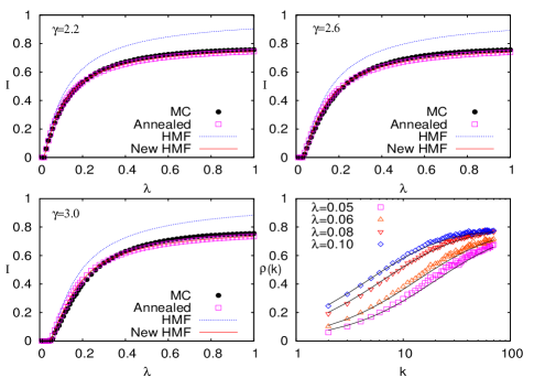
The most general network ensemble is provided by the configurational model configurational that generate a family of graphs by specifying a fixed degree sequence for the $N$ nodes, $\{k_{1},k_{2},...,k_{N}\}$. Each particular network realization is constructed by sorting each of the $L$ available links ($L=\sum_{i}k_{i}/2$). The probability that two nodes $i$ and $j$ are chosen to be connected in one network realization depends on their respective degrees as $k_{i}k_{j}/(2L^{2})$. Therefore, the probability that, after sorting the $L$ links, two given nodes $i$ and $j$ with degrees $k_{i}$ and $k_{j}$ are connected is ${\mathcal{A}}_{ij}={\mathcal{A}}_{ij}=k_{i}k_{j}/(2L)$. Now, inserting this latter AAM in eqs. 1 and 2 we can study the SIS dynamics of configurational ensembles. In Fig. 1 we represent the curves $I(\lambda)$ and the fraction of infected individuals with degree $k$, $\rho(k)$ obtained via the annealed formulation and the use of extensive numerical simulations of the SIS dynamics. The results of $I(\lambda)$ are shown for three families of configurational ensembles corresponding to $P(k)\sim k^{\gamma}$ with $\gamma=2.2$, $2.6$ and $3.0$. The network realizations used for the numerical simulations were constructed using the method introduced in PRE05 so to assure that no degree-degree correlations are present in any of the networks generated. As shown in Fig. 1, the results obtained using the AAM strongly agree with those obtained through extensive numerical simulations.

Figure 1: The top and bottom left panels show the phase diagrams, $I(\lambda)$, for the numerical simulations (points), the annealed formalism (squares), the usual (dashed line) and the new (solid line) HMF approximation. The networks have been constructed using the configurational model as introduced in PRE05 with degree sequences following power-law degree distributions, $P(k)\sim k^{-\gamma}$, with $\gamma=2.2$, $2.6$ and $3.0$. The networks have $N=5000$ and $\langle k\rangle=4$ and the statistics of the numerical simulations is made over $500$ network realizations for each value of $\lambda$. Besides, the bottom right panel show the fraction of infected nodes of degree $k$, $\rho(k)$, using numerical simulations (points) and the annealed formalism for the case $\gamma=2.2$ and several values of $\lambda$. The recovery probability is set to $\mu=0.3$.

We have compared the results of the AAM formulation with those obtained with the HMF. Surprisingly, the HMF fails to reproduce the phase diagrams $I(\lambda)$ as observed in Fig. 1. The reason of these discrepancies can be explained with the annealed formulation of the SIS dynamics. Taking the continuous-time formulation and assuming that all the nodes with the same degree have the same probability of being healthy, i.e. $s_{i}=\rho_{k}$ $\forall i$ with $k_{i}=k$, we can derive a new HMF approximation from eqs. (1) and the expression of ${\mathcal{A}}_{ij}$:

$$\dot{\rho}_{k}=\mu\left(1-\rho_{k}\right)-\rho_{k}\left[1-\prod_{k^{{}^{\prime}}}\left[1-\lambda\frac{kk^{{}^{\prime}}}{2L}(1-\rho_{k^{{}^{\prime}}})\right]^{N_{k^{{}^{\prime}}}}\right]$$ (3)

where $N_{k}=NP(k)$. This new HMF approximation when integrated for the different model networks perfectly reproduces the annealed approximation in contrast with the usual HMF approximation extensively used in network epidemiology up to date HMF1 ; HMF2 ; HMF3 .

The natural extension of eqs. (3) and (4) to general network models is done by considering that the probability of finding two nodes of degrees $k$ and $k^{{}^{\prime}}$ in the configurational model, $P(k^{{}^{\prime}},k)=kk^{{}^{\prime}}/2L$, reads as $P(k^{{}^{\prime}},k)=kP(k^{{}^{\prime}}|k)/(NP(k^{\prime}))$ for general network models. Then, we can write the new HMF as:

$$\dot{\rho}_{k}=\mu\left(1-\rho_{k}\right)-\rho_{k}\left[1-\prod_{k^{{}^{\prime}}}\left[1-\lambda\frac{kP(k^{{}^{\prime}}|k)}{N_{k^{{}^{\prime}}}}(1-\rho_{k^{{}^{\prime}}})\right]^{N_{k^{{}^{\prime}}}}\right]$$ (4)

Note that the new HMF formulation takes the form of the usual HMF equations only when $\lambda(1-\rho_{k})\ll 1$ $\forall k$:

$$\dot{\rho}_{k}\simeq\mu\left(1-\rho_{k}\right)-\lambda k\rho_{k}\sum_{k^{{}^{\prime}}}P(k^{{}^{\prime}}|k)(1-\rho_{k^{{}^{\prime}}})+{\cal O}(\lambda^{2})$$ (5)

Therefore, the usual HMF is only correct for $\lambda$ values before and around the epidemic onset (as observed from Fig. 1).

Now we describe the case of ensembles of networks constructed via attachment processes. In this case, network realizations are usually assembled by starting (at $\tau=0$) from a small graph of $m_{0}$ nodes coupled all-to-all. Therefore, the AAM has ${\mathcal{A}}_{ij}=1$ for $i$ and $j=1$, …, $m_{0}$ provided $i\neq j$ and ${\mathcal{A}}_{ii}=0$ otherwise. At each step $\tau$ of the network growth ($\tau=1$,…,$N-m_{0}$) a new node is added and launches $l$ links to the nodes of the network. Each of these nodes have some attachment probability, $\Pi_{i}(\tau)$ ($i=1$,…,$\tau+m_{0}-1$), of receiving one of the $l$ links from the new node. Therefore, the remaining $(N^{2}-m_{0}^{2})$ terms of the AAM read ${\mathcal{A}}_{ij}=1-(1-\Pi_{m}(M))^{l}$ (where $m=\min(i,j)$ and $M=\max(i,j)$) when $i\neq j$, and ${\mathcal{A}}_{ii}=0$ otherwise. Once the AAM is constructed one can obtain the annealed degree of the nodes as $k_{i}=\sum_{j}{\mathcal{A}}_{ij}$.

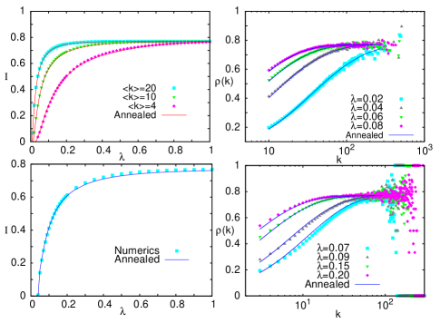
The networks grown through attachment processes are know to have nontrivial node-to-node correlations (e.g. age correlations) that play a key role in their dynamical behavior and are difficult to capture via HMF formulations. Now we show that these peculiarities of the attachment ensembles are captured by the annealed formulation of the SIS dynamics. Let us focus on the preferential attachment kernel introduced by Barabási and Albert (BA), $\Pi_{i}(\tau)=k_{i}(\tau)/\sum_{j}k_{j}(\tau)$ BA . In this case the networks have a power law degree distribution, $P(k)\sim k^{-3}$, and average degree $\langle k\rangle=2m$. Thus, by fixing the value of $m$ we can construct an ensemble of BA networks with the same values of $\langle k\rangle$. In Fig. 2 we show the results of $I(\lambda)$ and $\rho(k)$ by solving equations 1 with the expression of ${\cal A}_{ij}$ corresponding to three BA ensembles with $m=2$, $5$ and $10$. Again, the results of the AAM approximation show a perfect agreement with those obtained by means of numerical simulations of the SIS dynamics on top of BA networks.

Figure 2: (Top) In the left we show the epidemic phase diagram $I(\lambda)$ for three BA ensembles with $\langle k\rangle=4$, $10$ and $20$. In the right we show the fraction of infected individuals across degree-classes $\rho(k)$ for the ensemble with $\langle k\rangle=4$ and for different values of $\lambda$. The points correspond to numerical simulations of the SIS dynamics on top of $500$ network realizations while curves stand for the annealed approximation. The size of the networks is $N=5000$. (Bottom) Again, we show both $I(\lambda)$ (left) and $\rho(k)$ (right) for the case of adaptive growing networks when $N=10^{4}$. Both results of numerically grown networks (points), averaged over $5000$ realizations, and the solutions of the annealed formalism (curves) are shown. The network development is characterized by $\mu=0.3$, $\tau_{T}=1$ and $l=3$.

Now we focus on a more complicated attachment kernel describing a network growth interplaying with the internal dynamics of the nodes. In particular, the two entangled processes (network growth and system’s dynamics) coevolve in such a way that the attachment preferences of newcomers are driven by the dynamical states of their predecessors. Therefore, the attachment probability of a node $i$ at time $t>i$, $\Pi_{i}(t)$ depends, not only on the topological properties of node $i$, but also on its instant dynamical state $x_{i}(t)$. In our case $x_{i}(t)=s_{i}(t)$ and the attachment kernel reads: $\Pi_{i}(t)=k_{i}(t)s_{i}(t)/\sum_{j}k_{j}(t)s_{j}(t)$. This particular kernel couples networks growth and SIS dynamics so that newcomers prefer acquaintances with both structural importance and a healthy state. Therefore, infected nodes cannot receive a link from newcomers until they recover, whereas those healthy elements compete with each other according to their degrees as in the preferential attachment model.

The study of the above adaptive growth mechanism can be efficiently tackled with the help of the annealed formulation. To this aim we consider again the Markov SIS equations (1) incorporating a time-dependent AAM, ${\mathcal{A}}(t)$, in equation (2) that evolves simultaneously to the disease spreading. The initial condition of the AAM is set to ${\mathcal{A}}_{ij}(0)=1$ for $i,j\leq m_{0}$, $i\neq j$ and ${\mathcal{A}}_{ij}=0$ otherwise, while the dynamical state of the nodes is initialized as: $s_{i}(0)=1-I_{0}$ when $i\leq m_{0}$ and $s_{i}(0)=1$ otherwise. Then, we couple equations (1) with the evolution of the AAM:

$${\mathcal{A}}_{ij}(t)=H(t-\tau_{T}M)\left[1-(1-\Pi_{m}(\tau_{T}M))^{l}\right]\;,$$ (6)

when $i\neq j$ and $A_{ii}=0$ otherwise. The function $H(x)$ is the Heaviside step function so that the above equations state that the element ${\mathcal{A}}_{ij}$ has a zero value until the youngest element $M$ is incorporated. At this step, $t=\tau_{T}M$, the value of ${\mathcal{A}}_{ij}$ jumps to a stationary value that only depends on the attachment probability of the oldest node $m$ at time $M$.

Figure 3: Accumulated degree distribution of growing adaptive networks when $N=10^{4}$. The numerical results (points) and the distribution obtained from the evolution of the AAM (curves) are shown for several values of $\lambda$. The networks are grown using $\tau_{T}=1$, $l=3$ and $\mu=0.3$. Numerical results are obtained averaging over $100$ network realizations for each value of $\lambda$.

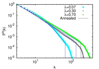
Iterating the above dynamics until the system size have reached a large enough value $N$ (so that it has reached a stationary regime for its intensive observables) we can evaluate the asymptotic impact of the disease and the structural properties of the generated networks. First, in Fig. 2 we show the phase diagram $I(\lambda)$ and the microscopic distribution of infected nodes across degree-classes, $\rho(k)$. Both measures clearly show the accuracy of the annealed approximation when compared to the results obtained averaging over a number of numerically grown networks. Besides, in Fig. 3 we show the corresponding accumulated degree distributions of the grown networks using different infection probabilities $\lambda$. From the figure we show that the AAM generated reproduces correctly the degree distributions obtained numerically. In particular, it is shown that for small values of $\lambda$ rather homogeneous networks are obtained, pointing out that the prevalence of disease on network hubs, as shown in Fig. 2 (bottom right panel), screens their fitness to attract new links and thus avoids the development of degree heterogeneity. On the contrary, for large $\lambda$ the disease affects homogeneously the forming system and newcomers mainly guide their links towards large degree nodes, thus recovering the behavior of the BA preferential attachment model.

Summing up, in this Letter we have shown that the dynamical behavior of static and adaptive networks can be efficiently described by the use of an unifying framework: the annealed formulation of the adjacency matrix. In both cases, the annealed formulation allows to compute the macroscopic observables and the microscopic distributions of the dynamics of a network ensemble in one single computation, thus avoiding the need of extensive simulations. In the case of adaptive networks, the treatment of the AAM as a dynamical object allows a simple formulation of the coupled structure-function problem. Particularizing to the case of SIS disease spreading on top of static networks, we have shown that the HMF approximation does not reproduces the phase diagram. Moreover, using the annealed formulation of the dynamics we have obtained a new HMF formulation that shows, for the first time, an accurate agreement with the numerical results. The use of the annealed formulation in other kind of network dynamics only requires to substitute the usual adjacency matrix by the AAM in the microscopic equations at work. Therefore, the formalism allows to write down explicitly the evolution equations for a wide variety of network ensembles, adaptive schemes and dynamics, regardless of their stochastic (e.g. contact processes, information diffusion, evolutionary dynamics, etc) or deterministic (e.g. nonlinear dynamical systems) nature. Although more research is needed to assess to what extent this approach can be such an important improvement in other dynamic network models, we expect that the annealed formulation will allow to tackle several open problems on networks dynamics and will pave the way to the theoretical studies of the growing field of complex adaptive systems.