Phase transitions and gaps in quantum random energy models

Abstract

By using a previously established exact characterization of the ground state of random potential systems in the thermodynamic limit, we determine the ground and first excited energy levels of quantum random energy models, discrete and continuous. We rigorously establish the existence of a universal first order quantum phase transition, obeyed by both the ground and the first excited states. The presence of an exponentially vanishing minimal gap at the transition is general but, quite interestingly, the gap averaged over the realizations of the random potential is finite. This fact leaves still open the chance for some effective quantum annealing algorithm, not necessarily based on a quantum adiabatic scheme.

1 Introduction

The perspective to realize a physical device representing a quantum computer (QC) has motivated a fervent research activity concerning the algorithms that could best exploit the intrinsic quantum properties of such a machine as opposed to the classical ones of current computers. In particular, there has been a growing interest toward the possibility to use quantum annealing (QAn) [1, 2, 3] as an alternative to simulated thermal annealing [4]. A pictorial viewpoint in fact suggests that in order to get the ground state (GS) of a given classical Hamiltonian $\bm{V}$, the thermal fluctuations, introduced to avoid the system to be trapped in local minima, could be replaced by quantum fluctuations able to outperform the former due to tunneling effects. Usually, QAn is associated with quantum adiabatic (QAd) algorithms [5, 6, 7]. The idea is to implement an interpolating Hamiltonian $\bm{H}(\Gamma)=\bm{V}+\Gamma\bm{K}$, where $\bm{K}$ is an operator which does not commute with $\bm{V}$. The adiabatic theorem ensures that for sufficiently slow changes of the parameter $\Gamma$ the interpolating system remains in its GS so that the original GS of $\bm{V}$ can be recovered in the limit $\Gamma\to 0$. However, for many interesting problems $\bm{V}$, the interpolating Hamiltonian $\bm{H}(\Gamma)$ is likely to undergo a first order quantum phase transition at some value $\Gamma=\Gamma_{\mathrm{c}}$, where the energy gap $\Delta$ between the first excited state (FES) and the GS becomes exponentially small in the system size $N$ [8, 9, 10]. In this case, a QAd decrease of $\Gamma$ starting from some value $\Gamma>\Gamma_{\mathrm{c}}$, where the GS of $\bm{H}(\Gamma)$ is found with ease, requires an exponentially long time. Otherwise, the system evolves into a combination of several instantaneous eigenstates of $\bm{H}(\Gamma)$ and when $\Gamma\to 0$ there is a finite probability to attain a state of $\bm{V}$ different from its GS. For $\bm{V}$ with a glassy energy landscape, “quantum is better” may be untrue [11].

The aim is this paper is threefold, we show that: (i) this phase transition scenario, characterized by a normal (paramagnetic) phase, for $\Gamma>\Gamma_{\mathrm{c}}$, and a condensed phase, for $\Gamma<\Gamma_{\mathrm{c}}$, is in fact universal, being valid for any hopping operator $\bm{K}$ and any potential operator $\bm{V}$; (ii) in the case of random potentials, where one must perform a quenched average over the different realizations of $\bm{V}$, or, instances, the average of the GS energy determines $\Gamma_{c}$ (see Eq. 2), the average of the gap remains finite and, with respect to $\Gamma$, is constant in the condensed phase, and linear in the normal phase; (iii) for any instance there exists a value $\Gamma_{\mathrm{min}}$ where the gap is exponentially small with the system size $N$, and $\Gamma_{\mathrm{min}}\to\Gamma_{\mathrm{c}}$ for $N\to\infty$. All the theoretical analysis is supported by unbiased numerical simulations. In the conclusions we shortly discuss the implications of points (i)-(iii) which make impossible to realize an efficient quantum adiabatic algorithm, but still leave open the chance for some effective more complicated quantum annealing scheme [12].

We analyze the case in which $\bm{V}$ is a generic random potential with a discrete or continuous distribution of the levels. For any choice of $\bm{K}$, provided that $\bm{K}$ has zero diagonal elements in the representation in which $\bm{V}$ is diagonal, $\bm{H}(\Gamma)=\bm{V}+\Gamma\bm{K}$ is a quantum random energy model (QREM) belonging to the class of systems studied in [13]. The term QREM refers to the quantum counterpart of the classical random energy model (REM), the model defined without the “hopping” operator $\bm{K}$, namely, $\bm{H}=\bm{V}$. In its original version, the REM was proposed with $\bm{V}$ having Gaussian distributed levels and represents a well known toy model for spin glasses [14]. The corresponding QREM has been first studied perturbatively and numerically in [8].

In Ref. [13] we have exactly characterized the GS and found a sufficient condition for the existence of a first order quantum phase transition for systems in which $\bm{V}$ is an arbitrary random potential. Here, we extend these results to study in detail both the GS and the FES energies of a generic QREM.

2 Ground state of random potential systems

In [13] we have determined the exact GS of a class of Hamiltonian models defined by an arbitrary hopping operator $\bm{K}$, i.e., an off diagonal matrix of dimension $M$, and a random potential $\bm{V}$, i.e., a diagonal matrix with $M$ i.i.d. random values $V$ extracted according to an arbitrary probability distribution $P(V)$. As usual, we will denote the system corresponding to a particular realization of the $V$ values as an instance and $\mathsf{E}(\cdot)=\int\cdot\ P(V)\mathrm{d}{V}$ will stand for the expectation over all possible instances. For the mentioned class of models, in the thermodynamic limit the energy $E_{0}$ of the GS is related to the lowest level $E_{0}^{(0)}$ of the hopping operator by

$$\int\frac{P(V)}{E_{0}-V}\leavevmode\nobreak\ \mathrm{d}{V}=\frac{1}{E_{0}^{(0)}},\qquad E_{0}\leq\mathsf{E}(V_{(1)}),$$ (1)

where $\mathsf{E}(V_{(k)})$ is the expectation of the $k$-th order statistic associated with the distribution $P(V)$, i.e., the expectation of the $k$-th smallest value among the $M$ values of $V$ drawn according to $P(V)$ [15]. Note that, whereas $E_{0}^{(0)}$ is deterministic, $E_{0}$ is stochastic and Eq. (1) is actually an equation for the expectation $\textsf{E}(E_{0})$. However, we assume that $E_{0}$ is self-averaging and this justifies the above notation.

The derivation of Eq. (1) follows from an exact probabilistic representation of the time evolution of a quantum system in terms of a proper collection of independent Poisson processes [16, 17, 18]. In fact, by using this representation, the lowest eigenvalue of $\bm{H}=\bm{V}+\Gamma\bm{K}$ can be expressed as the solution of a scalar equation written in terms of the asymptotic probability density of the potential and hopping frequencies (frequencies of the values of $\bm{V}$ and $\bm{K}$ realized in the probabilistic representation of an infinitely long time evolution) [13]. It happens that, for the above mentioned class of systems with a random potential, as well as for the uniformly fully connected models, in the thermodynamic limit the asymptotic probability density of the potential and hopping frequencies is exactly given by a multinomial. The equation for the ground-state level of $\bm{H}$ then greatly simplifies and, in the thermodynamic limit, takes on the form of Eq. (1) [13]. We assume a non-trivial thermodynamic limit, namely, a limit in which the lowest levels of $\bm{H}$, $\bm{V}$ and $\bm{K}$ diverge with the same speed (the most interesting case being the one in which such levels are all extensive in $N$). Apart from this, the distribution $P(V)$ remains completely arbitrary.

Equation (1) has a simple interpretation: the average of the inverse hopping energy, estimated as $1/(E_{0}-V)$, must coincide with the inverse of the actual hopping energy, namely, $1/E_{0}^{(0)}$, with the constraint that $E_{0}$ does not exceed the averaged minimum potential. It may happen that the solution of the integral problem in Eq. (1) becomes incompatible with the constraint $E_{0}\leq\mathsf{E}(V_{(1)})$. This may occur, for instance, when some parameter of the model is changed below a threshold, e.g., $\Gamma<\Gamma_{\mathrm{c}}$ for the Hamiltonian $\bm{H}(\Gamma)=\Gamma\bm{K}+\bm{V}$. Then, the GS of an instance condensates, for $\Gamma<\Gamma_{\mathrm{c}}$, into the eigenstate of $\bm{V}$ corresponding to the minimum value $V$ realized in that instance. As a result, $E_{0}(\Gamma)=\mathsf{E}(V_{(1)})$ for any $\Gamma<\Gamma_{\mathrm{c}}$ and we obtain a condensation in the space of states [19]. Note that each instance condensates into a different state, however, this state corresponds, for all instances, to that of minimum potential. A sufficient condition for this first order quantum phase transition to take place is that $P(\mathsf{E}(V_{(1)}))\to 0$ in the thermodynamic limit [13].

When the above results are applied to a quantum mechanical model, $M$ stands for the dimension of the Fock space and, in general, we have $M\gg N$, where $N$ is the size (number of particles) of the system. The phase transition is determined by the condition $E_{0}=\mathsf{E}(V_{(1)})$, where $E_{0}$ is the solution of the integral problem in Eq. (1), namely

$$\int\frac{P(V)}{\mathsf{E}(V_{(1)})-V}\leavevmode\nobreak\ \mathrm{d}{V}=\frac{1}{E_{0}^{(0)}}.$$ (2)

This is the equation which allows us to find the critical point of the phase transition in terms of the “hopping” parameter $\Gamma$ or, possibly, in terms of other parameters contained in the probability distribution $P(V)$.

3 Discrete and continuous QREMs

Let us consider the Hamiltonian $\bm{H}=\Gamma\bm{K}+\bm{V}$ acting on the $M=2^{N}$ spin states

$$|\bm{n}\rangle=|n_{1},n_{2},\dots,n_{N}\rangle=|n_{1}\rangle\otimes|n_{2}\rangle\otimes\dots\otimes|n_{N}\rangle,$$ (3)

where $|n_{i}\rangle$, with $n_{i}=\pm 1$, is the eigenstate of the Pauli matrix $\sigma^{z}_{i}$ acting on the $i$-th spin and $i=1,\dots,N$, $\sigma^{z}_{i}|n_{i}\rangle=n_{i}|n_{i}\rangle$. The hopping operator $\bm{K}$ is chosen as the sum of single-flip operators

$$\bm{K}=-\sum_{i=1}^{N}\mathbbm{1}_{1}\otimes\ldots\otimes\mathbbm{1}_{i-1}\otimes\sigma^{x}_{i}\otimes\mathbbm{1}_{i+1}\dots\otimes\ldots\mathbbm{1}_{N},$$

$\sigma^{x}_{i}$ being the $x$ Pauli matrix acting on the $i$-th spin. More general forms for $\bm{K}$ can be considered and tackled in a similar way. The potential $\bm{V}$ is a diagonal operator with elements $V_{\bm{n}}=\langle\bm{n}|\bm{V}|\bm{n}\rangle$ which are i.i.d. random variables drawn with distribution $P(V)$. As an example of discrete QREMs we will consider the case in which $V$ takes the values $V_{k}=-J(N-2k)$, $k=0,1,\ldots,N$, with probability mass function $P(V_{k})=2^{-N}\binom{N}{k}$. We will refer to this model as the binomial QREM. As an example of continuous models we will assume $V\in(-\infty,+\infty)$ with probability density function $P(V)=(\pi NJ^{2})^{-1/2}\exp(-V^{2}/(NJ^{2}))$. We will refer to this model as the Gaussian QREM.

In the thermodynamic limit $N\to\infty$, the distribution $P(V)$ concentrates around some value $V_{\mathrm{sp}}$ where $P^{\prime}(V_{\mathrm{sp}})=0$ and $P^{\prime\prime}(V_{\mathrm{sp}})<0$. The integral in Eq. (1) can be then performed, exactly, by the saddle-point method, namely,

$$\int\frac{P(V)}{E_{0}-V}\mathrm{d}{V}=\frac{1}{E_{0}-V_{\mathrm{sp}}}.$$ (4)

For symmetric distributions, $P(-V)=P(V)$, we have $V_{\mathrm{sp}}=0$ and Eq. (1) amounts to $E_{0}=\min(E_{0}^{(0)},\mathsf{E}(V_{(1)}))$.

The spectrum of $\Gamma\bm{K}$ is trivial and, in particular, the GS level is $E_{0}^{(0)}=-\Gamma N$. Equation (1) thus provides

$$E_{0}=\left\{\begin{array}[]{ll}\mathsf{E}(V_{(1)})&\Gamma<\Gamma_{\mathrm{c}}\\ -\Gamma N&\Gamma\geq\Gamma_{\mathrm{c}}\end{array}\right.,$$ (7)

where, according to Eq. (2), $\Gamma_{\mathrm{c}}=\lim_{N\to\infty}-\mathsf{E}(V_{(1)})/N$. Stated in this form, the result applies to any QREM. In the binomial model $\mathsf{E}(V_{(1)})=-JN+O(1)$, whereas in the Gaussian model $\mathsf{E}(V_{(1)})=-JN\sqrt{\ln 2}+O(1)$. The critical hopping parameter separating the condensed and the normal phases is then $\Gamma_{\mathrm{c}}=J$ and $\Gamma_{\mathrm{c}}=J\sqrt{\ln 2}$, respectively.

By introducing auxiliary Hamiltonians, we can use again Eq. (1) to evaluate the eigenvalues of $\bm{H}$ corresponding to excited states. Suppose, to begin with, that we are in the condensed phase $\Gamma N<-\mathsf{E}(V_{(1)})$. For a given realization of the random potential $\bm{V}$, the GS of $\bm{H}$ is $|\bm{n}_{1}\rangle$, where $\bm{n}_{1}$ is the spin configuration associated with the smallest value of the potential, i.e., $V_{\bm{n}_{1}}=\min_{\bm{n}}V_{\bm{n}}$. For simplicity, we suppose that $V_{\bm{n}_{1}}$ is non-degenerate, a condition which is almost surely met in the Gaussian QREM. For $V_{\bm{n}_{1}}$ degenerate a similar argument applies. We then introduce the Hamiltonian

$$\tilde{\bm{H}}=\bm{H}-V_{\bm{n}_{1}}|\bm{n}_{1}\rangle\langle\bm{n}_{1}|,$$ (8)

whose lowest eigenvalue $\tilde{E}_{0}$ coincides with the level $E_{1}$ of $\bm{H}$. Note that $\tilde{\bm{H}}$ describes a system with random potential $\tilde{V}$ having distribution $\tilde{P}(\tilde{V})$ such that $\tilde{\mathsf{E}}(\tilde{V}_{(1)})=\mathsf{E}(V_{(2)})$. Moreover, the operators $\tilde{\bm{H}}$ and $\bm{H}$ have the same non-diagonal part, i.e., $\tilde{E}_{0}^{(0)}=E_{0}^{(0)}$. From Eq. (1) applied to the Hamiltonian $\tilde{\bm{H}}$ we thus find

$$\tilde{E}_{0}=\left\{\begin{array}[]{ll}\mathsf{E}(V_{(2)})&\Gamma<-\mathsf{E}(V_{(2)})/N\\ -\Gamma N&\Gamma\geq-\mathsf{E}(V_{(2)})/N\end{array}\right..$$ (11)

We proceed with a similar analysis in the normal phase. For $\Gamma N\gg-\mathsf{E}(V_{(1)})$, the GS of $\bm{H}$ approaches the GS of $\bm{K}$, namely $|0_{\bm{K}}\rangle=2^{-N/2}\sum_{\bm{n}}|\bm{n}\rangle$. Observing that $\mathsf{E}(\langle 0_{\bm{K}}|\bm{H}|0_{\bm{K}}\rangle)=-\Gamma N+\mathsf{E}(V)=-\Gamma N$ exactly for any $\Gamma$, we assume $|0_{\bm{K}}\rangle$ to represent an effective GS in all the normal region. We then introduce the Hamiltonian

$$\tilde{\bm{H}}=\bm{H}+\Gamma N|0_{\bm{K}}\rangle\langle 0_{\bm{K}}|,$$ (12)

which, we guess, in all the normal region, has the average lowest eigenvalue $\tilde{E}_{0}$ coincident with the average level $E_{1}$ of $\bm{H}$. We split $\tilde{\bm{H}}$ as

$$\tilde{\bm{H}}=\tilde{\bm{V}}+\Gamma\tilde{\bm{K}},$$ (13)

where $\tilde{\bm{V}}=\bm{V}+\Gamma N2^{-N}$ is a random potential with distribution $\tilde{P}(\tilde{V})=P(V)$, and $\tilde{\bm{K}}=\bm{K}+N2^{-N}(\bm{W}-\bm{1})$ a hopping operator with $\bm{W}$ defined by matrix elements $W_{\bm{n},\bm{n}^{\prime}}=1$. Let $|1_{\bm{K}}^{(i)}\rangle=\sigma_{i}^{z}|0_{\bm{K}}\rangle$, $i=1,\dots,N$, be the $N$-degenerate FESs of $\bm{K}$, namely, $\bm{K}|1_{\bm{K}}^{(i)}\rangle=-\Gamma(N-2)|1_{\bm{K}}^{(i)}\rangle$. Similarly, let $|2_{\bm{K}}^{(i,j)}\rangle=\sigma_{i}^{z}\sigma_{j}^{z}|0_{\bm{K}}\rangle$, $i,j=1,\dots,N$, with $i\neq j$, be the $N(N-1)/2$-degenerate second exited states of $\bm{K}$, namely, $\bm{K}|2_{\bm{K}}^{(i,j)}\rangle=-\Gamma(N-4)|2_{\bm{K}}^{(i,j)}\rangle$, and so on. By using $\bm{W}|0_{\bm{K}}\rangle=2^{N}|0_{\bm{K}}\rangle$ and $\bm{W}|1_{\bm{K}}^{(i)}\rangle=\bm{W}|2_{\bm{K}}^{(i,j)}\rangle=\ldots=0$, we find that any $|1_{\bm{K}}^{(i)}\rangle$ is a GS of $\tilde{\bm{K}}$ with eigenvalue $-(N-2)-N2^{-N}$. By inserting $\tilde{E}_{0}^{(0)}=-\Gamma(N-2+N2^{-N})$, and $\tilde{\mathsf{E}}(\tilde{V}_{(1)})=\mathsf{E}(V_{(1)})+\Gamma N2^{-N}$ into Eq. (1) for $\tilde{\bm{H}}$, we get

$$\tilde{E}_{0}=\left\{\begin{array}[]{ll}\mathsf{E}(V_{(1)})+\Gamma N2^{-N}&\Gamma<\frac{-\mathsf{E}(V_{(1)})}{N-2+N2^{-N}}\\ -\Gamma(N-2)&\Gamma\geq\frac{-\mathsf{E}(V_{(1)})}{N-2+N2^{-N}}\end{array}\right..$$ (16)

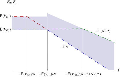
Finally, we combine Eqs. (11) and (16) to obtain $E_{1}$, see Fig. 1. Observing that $\lim_{N\to\infty}\left(\mathsf{E}(V_{(2)})-\mathsf{E}(V_{(1)})\right)/N=0$, we conclude that in the thermodynamic limit

$$E_{1}=\left\{\begin{array}[]{lr}\mathsf{E}(V_{(2)})&\Gamma<\Gamma_{\mathrm{c}}\\ -\Gamma(N-2)&\Gamma\geq\Gamma_{\mathrm{c}}\end{array}\right..$$ (19)

Equation (1) and hence $E_{0}$ and $E_{1}$ found above are exact up to terms $O(1)$ [13]. However, the $O(1)$ errors obtained for $E_{0}$ and $E_{1}$ match when $N\to\infty$. It follows that for $N\to\infty$ the average gap $\mathsf{E}(\Delta)=E_{1}-E_{0}$ is

$$\mathsf{E}(\Delta)=\left\{\begin{array}[]{ll}\mathsf{E}(V_{(2)})-\mathsf{E}(V_{(1)})&\Gamma<\Gamma_{\mathrm{c}}\\ 2\Gamma&\Gamma\geq\Gamma_{\mathrm{c}}\end{array}\right..$$ (22)

In the condensed phase, the average gap is a constant which amounts to $\mathsf{E}(\Delta)/J=2/e$ in the binomial QREM and $\mathsf{E}(\Delta)/J\simeq 0.62$ in the Gaussian QREM. These results immediately follow from the evaluation of the first two order statistics associated with the chosen $P(V)$. In the case of the binomial distribution, we have

$$\mbox{$\mathsf{E}$}(V_{(1)}) =-JN\mathrm{Prob}(V_{(1)}=-JN)$$

$$\quad-J(N-2)\mathrm{Prob}(V_{(1)}=-J(N-2))+\dots$$

$$=-JN+J\frac{2}{e},$$ (23)

$$\mbox{$\mathsf{E}$}(V_{(2)}) =-JN\mathrm{Prob}(V_{(2)}=-JN)$$

$$\quad-J(N-2)\mathrm{Prob}(V_{(2)}=-J(N-2))+\dots$$

$$=-JN+J\frac{4}{e},$$ (24)

where the probabilities have been estimated in the limit $N\to\infty$, namely,

$$\mathrm{Prob}(V_{(1)}=-JN)=1-\frac{1}{e},$$ (25)

$$\mathrm{Prob}(V_{(1)}=-J(N-2))=\frac{1}{e},$$ (26)

$$\mathrm{Prob}(V_{(2)}=-JN)=1-\frac{2}{e},$$ (27)

$$\mathrm{Prob}(V_{(2)}=-J(N-2))=\frac{2}{e}.$$ (28)

Note that, in this limit, $\mathrm{Prob}(V_{(1)}\geq-J(N-4))$ and $\mathrm{Prob}(V_{(2)}\geq-J(N-4))$ vanish. In the case of the Gaussian distribution, the $O(1)$ contributions to $\mathsf{E}(V_{(1)})$ and $\mathsf{E}(V_{(2)})$ have been evaluated numerically, the difference being close to $0.62\leavevmode\nobreak\ J$.

Figure 1: Lowest two energy levels $E_{0}$ and $E_{1}$ (bottom and top edges of the shaded area, respectively) for a QREM in the thermodynamic limit as a function of the hopping parameter $\Gamma$. The blue long-dashed line is the value of $E_{0}$ given by Eq. (7), whereas the red medium-dashed and green short-dashed lines represent the finite-$N$ estimate for $E_{1}$ given by Eqs. (11) and (16), respectively. As $N\to\infty$ the critical points (corresponding to the dotted vertical lines) concur at $\Gamma_{\mathrm{c}}=-\mathsf{E}(V_{(1)})/N$ where $E_{1}$ develops a $O(1)$ discontinuity.

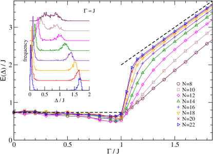
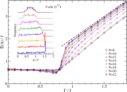
The results of Eqs. (7), (19) and (22) have been compared with those from exact numerical diagonalizations of $\bm{H}$ for different values of the system size $N$. In Figs. 2 and 3 we show the behavior of the average gap in the binomial and Gaussian QREMs, respectively. In both cases the data obtained for $N$ from 8 to 22 exhibit a systematic convergence toward the thermodynamic limit (22).

Figure 2: Average gap $\mathsf{E}(\Delta)$ in the binomial QREM as a function of $\Gamma$ for different system sizes $8\leq N\leq 22$. The dashed line is the predicted value in the thermodynamic limit whereas for each size $N$ the symbols joined by straight lines are the averages from exact numerical diagonalization of 1000 instances. Inset: histograms of the frequencies of the gap values evaluated at $\Gamma=\Gamma_{\mathrm{c}}$ (size $8\leq N\leq 22$ from top to bottom, curves shifted for the sake of clarity).

Figure 3: As in Fig. 2 for the Gaussian QREM.

Our numerical data confirm that, as usually assumed, the extensive quantities $E_{0}$ and $E_{1}$ are self-averaging. For the gap, on the other hand, we observe a different behavior. In the normal phase, $\Delta$ is self-averaging whereas this property is lost when the system condensates. In the insets of Fig. 2 and 3 we show the frequencies of the gap values at the critical point $\Gamma=\Gamma_{\mathrm{c}}$ for the binomial and Gaussian QREMs, respectively. These frequencies, evaluated from a set of 1000 instances, have been checked to be a good approximation of the exact distributions of $\Delta$ at the chosen sizes $N$. It is evident that $\lim_{N\to\infty}\mathrm{var}(\Delta)/\mathsf{E}(\Delta)^{2}\neq 0$, i.e., $\Delta$ is not self-averaging. The same conclusion is reached for both binomial and Gaussian QREMs in the whole range $0\leq\Gamma\leq\Gamma_{\mathrm{c}}$.

The gap distributions for the binomial and the Gaussian QREMs have well distinct shapes in the condensed phase. In the discrete model, when $\Gamma$ is decreased below $\Gamma_{\mathrm{c}}$ the gap values concentrate around $\Delta=0,2J,4J,\dots$. Including only terms not vanishing in the limit $N\to\infty$, at $\Gamma=0$ the gap distribution becomes $q_{N}(\Delta)=r_{N}\delta(\Delta)+(1-r_{N})\delta(\Delta-2J)$, where $r_{N}$ can be calculated analytically and for $N$ large approaches $1-1/e$. This behavior is qualitatively not different from that shown in the inset of Fig. 2 for $\Gamma=\Gamma_{\mathrm{c}}$. In the continuous model, the gap values are evenly distributed in the range $0\leq\Delta\leq 2\Gamma_{\mathrm{c}}$ for $\Gamma\lesssim\Gamma_{\mathrm{c}}$. The distribution smoothly deforms by decreasing $\Gamma$ and at $\Gamma=0$ is exactly described by the function

$$q_{N}(\Delta)=\ \theta(\Delta)\frac{2^{N}(2^{N}-1)}{\pi\sqrt{NJ^{2}}}\int_{-\infty}^{+\infty}e^{-t^{2}-(t+\Delta/\sqrt{NJ^{2}})^{2}}$$

$$\times[\mathrm{Erfc}(t+\Delta/\sqrt{NJ^{2}})/2]^{2^{N}-2}\mathrm{d}{t}.$$ (29)

The logarithm of (29) is well approximated by the first two terms of its Taylor expansion at $\Delta=0$. By using the normalization condition, we then have $q_{N}(\Delta)\simeq q_{N}(0)\exp[-q_{N}(0)\Delta]$, where $q_{N}(0)$ quickly saturates for $N\to\infty$ to a constant value near $1/\mathsf{E}(\Delta)=1/(0.62\leavevmode\nobreak\ J)$.

4 Minimal gap

It is interesting to understand how the flat trend of $\mbox{$\mathsf{E}$}(\Delta)$ observed in the whole condensed region, is attained from the actual behavior of the gap of the single instances. In fact, at least for the Gaussian QREM, it has been shown by numerical and theoretical arguments [8], as well as rigorously demonstrated [10], that, close to the critical point, the gap of each single instance has a rather different behavior: it vanishes exponentially by increasing the size $N$.

Figure 4: Gap $\Delta$ of an instance as a function of $\Gamma$ for a Gaussian QREM model with $N=20$ spins. Similar results are obtained for a binomial QREM.

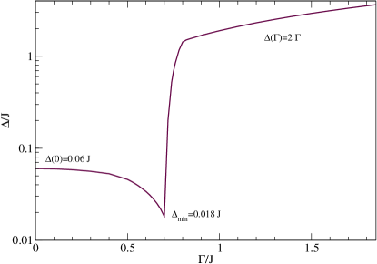
In fact, for any instance of size $N$, by varying $\Gamma$ the gap $\Delta(\Gamma)$ has a minimum at $\Gamma=\Gamma_{\textrm{min}}$ as shown in Fig. 4. Let us define $\Delta_{\textrm{min}}=\min_{\Gamma\geq 0}\Delta(\Gamma)$. Theoretical arguments, checked numerically for both Gaussian and binomial QREMs, show that (a) $\Delta_{\textrm{min}}$ and $\Gamma_{\textrm{min}}$ are self-averaging quantities, (b) $\mathsf{E}(\Delta_{\textrm{min}})\simeq 2\Gamma_{\mathrm{c}}N2^{-N/2}$ for $N$ large and (c) $\lim_{N\to\infty}\mathsf{E}(\Gamma_{\textrm{min}})=\Gamma_{\mathrm{c}}$ with $\mathrm{var}(\Gamma_{\textrm{min}})\simeq(\Gamma_{\mathrm{c}}/N)^{2}$ for $N$ large.

In principle, the shape of $\Delta(\Gamma)$ for a given instance can be accurately reproduced by the variational Ritz method writing the lowest eigenstates of $\bm{H}(\Gamma)$, $|E_{n}(\Gamma)\rangle$ with $n=0,1$, as a superposition of the lowest eigenstates of $\bm{K}$ and $\bm{V}$. In the crudest approximation, namely,

$$|E_{n}(\Gamma)\rangle=a_{n}(\Gamma)|0_{\bm{K}}\rangle+b_{n}(\Gamma)|\bm{n}_{1}\rangle,$$ (30)

by using $\langle 0_{\bm{K}}|V|0_{\bm{K}}\rangle=0$, valid whenever $P(-V)=P(V)$, one obtains the analytical estimate

$$\Delta(\Gamma)=\sqrt{(N\Gamma+V_{\bm{n}_{1}})^{2}-4N\Gamma V_{\bm{n}_{1}}2^{-N}},$$ (31)

which gives

$$\Gamma_{\mathrm{min}}=-V_{\bm{n}_{1}}/N$$ (32)

and

$$\Delta_{\mathrm{min}}=-2V_{\bm{n}_{1}}2^{-N/2}.$$ (33)

Properties (a), (b) and (c) follow straightaway from these two expressions observing that $V_{\bm{n}_{1}}=V_{(1)}$ and, for $N\to\infty$, $\mathsf{E}(V_{(1)})=-\Gamma_{\mathrm{c}}N+O(1)$, whereas $\mathrm{var}(V_{(1)})$ approaches a constant value close to $\Gamma_{\mathrm{c}}^{2}$.

We are now in a position to discuss how the results of Figs. 2 and 3 are recovered from the behavior of the gap of the individual instances.

In the region $\Gamma<\Gamma_{\mathrm{c}}$, where the gap is not self-averaging, $\mathsf{E}(\Delta)$ must loose memory of the instance-dependent minimum of $\Delta$. Close to the critical point, this is quantitatively understood as follows. For $N$ large and $\Gamma\simeq\Gamma_{\mathrm{min}}=-\mbox{$\mathsf{E}$}(V_{(1)})/N$, according to Eq. (31), we have $\Delta\simeq|-\mbox{$\mathsf{E}$}(V_{(1)})+V_{(1)}|$. We have to average this expression over all values of $V_{(1)}$. For the Gaussian QREM, neglecting large deviatons, the probability distribution of $V_{(1)}$ is well approximated by a Gaussian centered at $\mbox{$\mathsf{E}$}(V_{(1)})$ with variance $\mathrm{var}(V_{(1)})$. We thus have

$$\mbox{$\mathsf{E}$}(\Delta) \simeq\int_{-\infty}^{+\infty}|-\mbox{$\mathsf{E}$}(V_{(1)})+V_{(1)}|\frac{e^{-\frac{(V_{(1)}-\mathsf{E}(V_{(1)}))^{2}}{2\mathrm{var}(V_{(1)})}}}{\sqrt{2\pi\mathrm{var}(V_{(1)})}}\mathrm{d}{V_{(1)}}$$

$$=\sqrt{\frac{2}{\pi}\mathrm{var}(V_{(1)})}.$$ (34)

We numerically find $\mathrm{var}(V_{(1)})\simeq 0.611J^{2}$, therefore, this result is in very good agreement with the value $\mbox{$\mathsf{E}$}(V_{(2)})-\mbox{$\mathsf{E}$}(V_{(1)})$ of Eq. (22), valid in the whole condensed region. For the binomial QREM, we can use the probabilities (25) and (26) to obtain the exact result

$$\mbox{$\mathsf{E}$}(\Delta) =|-\mbox{$\mathsf{E}$}(V_{(1)})-JN|\mathrm{Prob}(V_{(1)}=-JN)$$

$$\quad+|-\mbox{$\mathsf{E}$}(V_{(1)})-J(N-2)|\mathrm{Prob}(V_{(1)}=-J(N-2))$$

$$=J\frac{2}{e}.$$ (35)

Note that the distribution functions of $\Delta$ achievable from Eqs. (34) and (35) are in qualitative agreement, in particular, they confirm the non self-averaging character of $\Delta$, with the frequencies of the gap values at $\Gamma=\Gamma_{\mathrm{c}}$ shown in Figs. 2 and 3 for finite sizes $N$.

Vice versa, the self-averaging property of the gap in force for $\Gamma>\Gamma_{\mathrm{c}}$ implies that, for almost any instance, $\Delta\simeq\mathsf{E}(\Delta)$ changes smoothly, at finite $N$, between its value in the condensed region and the normal phase behavior $\Delta(\Gamma)=2\Gamma$ (exact in the thermodynamic limit or for $\Gamma\gg\Gamma_{\mathrm{c}}$), see Figs. 2 and 3. According to Eq. (16) and in agreement with the numerical simulations, this change takes place in the interval $\Gamma_{\mathrm{min}}\leq\Gamma\leq\Gamma_{\mathrm{min}}+2\Gamma_{\mathrm{c}}/(N-2)$. Equation (31) clearly fails in describing this behavior. We have to resort to a more consistent variational analysis including a superposition of the lowest eigenstates of $\bm{K}$, namely, $|0_{\bm{K}}\rangle$ and $|1_{\bm{K}}^{(i)}\rangle$, $i=1,\dots,N$, and of several lowest eigenstates of $\bm{V}$, $|\bm{n}_{l}\rangle$ with $l=1,2,\dots$. Numerical results, not reported here, show that this analysis is able to capture the quantitative behavior of the gap of each single instance. A crucial point, still to be understood, is how the effective number of lowest $\bm{V}$ eigenstates to be included in this analysis scales with the size $N$.

5 Conclusions

All QREM models are characterized by a universal phase transition between a condensed phase and a normal one, the critical point $\Gamma_{\mathrm{c}}$ being the solution of Eq. (2). The gap averaged over the $\bm{V}$ realizations is finite, and undergoes the same phase transition, being constant for $\Gamma<\Gamma_{\mathrm{c}}$, and growing linearly in $\Gamma$ for $\Gamma>\Gamma_{\mathrm{c}}$ (more precisely, as $2\Gamma$, the gap of the system with $\bm{V}\equiv 0$). The existence, for each $\bm{V}$ realization, of a minimal gap at $\Gamma=\Gamma_{\mathrm{c}}$ exponentially small in the system size $N$, implies that, QAd algorithms (at real or imaginary times) aimed at finding the configuration of minimal potential, would require a computational time $t>\Delta_{\textrm{min}}^{-1}$ exponentially long with $N$ for almost any instance. In principle, by exploiting the fact that the average gap is finite, one can hope to elude this limitation by using an adiabatic path across the $\bm{V}$ ensemble in which the transit through a gap minimum is avoided [12]. However, it is not clear how to realize this path for $\bm{V}$ of the class considered here.

Another possibility is the realization of a partial QAd algorithm, which has the purpose of selecting not the actual lowest eigenstate of $\bm{V}$ but a set of lowest eigenstates, from which the lowest one can be found by probabilistic methods. Of course, the success of this approach depends on the scaling properties of the number of these eigenstates with respect to the size $N$ of the system.

References

- Apolloni et al. [1989] B. Apolloni, C. Carvalho, D. de Falco, Quantum stochastic optimization, Stochastic Processes and their Applications 33 (1989) 233 – 244.
- Finnila et al. [1994] A. B. Finnila, M. A. Gomez, C. Sebenik, C. Stenson, J. D. Doll, Quantum annealing: A new method for minimizing multidimensional functions, Chemical Physics Letters 219 (1994) 343 – 348.
- Kadowaki and Nishimori [1998] T. Kadowaki, H. Nishimori, Quantum annealing in the transverse ising model, Phys. Rev. E 58 (1998) 5355–5363.
- Kirkpatrick et al. [1983] S. Kirkpatrick, C. D. J. Gelatt, M. P. Vecchi, Optimization by Simulated Annealing, Science 220 (1983) 671–680.
- Farhi et al. [2000] E. Farhi, J. Goldstone, S. Gutmann, M. Sipser, Quantum Computation by Adiabatic Evolution, 2000.
- Farhi et al. [2001] E. Farhi, J. Goldstone, S. Gutmann, J. Lapan, A. Lundgren, D. Preda, A Quantum Adiabatic Evolution Algorithm Applied to Random Instances of an NP-Complete Problem, Science 292 (2001) 472–475.
- Santoro and Tosatti [2006] G. E. Santoro, E. Tosatti, Optimization using quantum mechanics: quantum annealing through adiabatic evolution, Journal of Physics A: Mathematical and General 39 (2006) R393.
- Jörg et al. [2008] T. Jörg, F. Krzakala, J. Kurchan, A. C. Maggs, Simple glass models and their quantum annealing, Phys. Rev. Lett. 101 (2008) 147204.
- Jörg et al. [2010] T. Jörg, F. Krzakala, J. Kurchan, A. C. Maggs, J. Pujos, Energy gaps in quantum first-order mean-field–like transitions: The problems that quantum annealing cannot solve, EPL (Europhysics Letters) 89 (2010) 40004.
- Adame and Warzel [2015] J. Adame, S. Warzel, Exponential vanishing of the ground-state gap of the quantum random energy model via adiabatic quantum computing, Journal of Mathematical Physics 56 (2015).
- Battaglia et al. [2005] D. A. Battaglia, G. E. Santoro, E. Tosatti, Optimization by quantum annealing: Lessons from hard satisfiability problems, Phys. Rev. E 71 (2005) 066707.
- Farhi et al. [2009] E. Farhi, J. Goldstone, D. Gosset, S. Gutmann, H. B. Meyer, P. Shor (2009).
- Ostilli and Presilla [2006] M. Ostilli, C. Presilla, The exact ground state for a class of matrix hamiltonian models: quantum phase transition and universality in the thermodynamic limit, Journal of Statistical Mechanics: Theory and Experiment 2006 (2006) P11012.
- Derrida [1980] B. Derrida, Random-energy model: Limit of a family of disordered models, Phys. Rev. Lett. 45 (1980) 79–82.
- Johnson et al. [2005] N. L. Johnson, A. W. Kemp, S. Kotz, Univariate Discrete Distributions, Wiley, 3rd edition edition, 2005.
- De Angelis et al. [1983] G. F. De Angelis, G. Jona-Lasinio, M. Sirugue, Probabilistic solution of pauli type equations, Journal of Physics A: Mathematical and General 16 (1983) 2433.
- De Angelis et al. [1998] G. F. De Angelis, G. Jona-Lasinio, V. Sidoravicius, Berezin integrals and poisson processes, Journal of Physics A: Mathematical and General 31 (1998) 289.
- Beccaria et al. [1999] M. Beccaria, C. Presilla, G. F. De Angelis, G. Jona-Lasinio, An exact representation of the fermion dynamics in terms of poisson processes and its connection with monte carlo algorithms, EPL (Europhysics Letters) 48 (1999) 243.
- Ostilli and Presilla [2017] M. Ostilli, C. Presilla, First-order quantum phase transitions as condensations in the space of states, arXiv:1712.05294 (2017).