Computationally Efficient Estimation of Factor Multivariate Stochastic Volatility Models
Abstract
An Markov chain Monte Carlo simulation method based on a two stage delayed rejection Metropolis-Hastings algorithm is proposed to estimate a factor multivariate stochastic volatility model. The first stage uses ‘-step iteration’ towards the mode, with small, and the second stage uses an adaptive random walk proposal density. The marginal likelihood approach of Chib (1995) is used to choose the number of factors, with the posterior density ordinates approximated by Gaussian copula. Simulation and real data applications suggest that the proposed simulation method is computationally much more efficient than the approach of Chib et al. (2006). This increase in computational efficiency is particularly important in calculating marginal likelihoods because it is necessary to carry out the simulation a number of times to estimate the posterior ordinates for a given marginal likelihood. In addition to the Markov chain Monte Carlo method, the paper also proposes a fast approximate EM method to estimate the factor multivariate stochastic volatility. The estimates from the approximate EM method are of interest in their own right but are especially useful as initial inputs to Markov chain Monte Carlo methods, making them more efficient computationally. The methodology is illustrated using simulated and real examples.
Key words: Approximate EM, Adaptive sampling, Delayed rejection, Gaussian copula, marginal likelihood, Markov chain Monte Carlo
JEL Classification: C11, C15, C32
1 Introduction
Factor multivariate stochastic volatility (factor MSV) models are increasingly used in the financial economics literature because they can model the volatility dynamics of a large system of financial and economic time series when the common features in these series can be captured by a small number of latent factors. These models naturally link in with factor pricing models such as the arbitrage pricing theory (APT) model of Ross (1976), which is built on the existence of a set of common factors underlying all asset returns, and the capital asset pricing model (CAPM) of Sharpe (1964) and Lintner (1965) where the ‘market return’ is the common risk factor affecting all the assets. However, unlike factor MSV models, standard factor pricing models usually do not attempt to model the dynamics of the volatilities of the asset returns and instead assume the second moments are constant. Factor MSV models have recently been applied to important problems in financial markets such as asset allocation (e.g. Aguilar and West, 2000; Han, 2006) and asset pricing (e.g. Nardari and Scruggs, 2006). Empirical evidence suggests that factor MSV models are a promising approach for modeling multivariate time-varying volatility, explaining excess asset returns, and generating optimal portfolio strategies.
A computationally efficient method of estimating a high dimensional dynamic factor MSV model is necessary if such a model is to be applied to financial problems to make decisions in a timely way. For example, when new information becomes available to financial markets, fund managers need to quickly incorporate it into their portfolio strategies, so the speed with which a factor MSV can be re-estimated is an important practical issue. However, based on results reported in the literature (e.g. Chib et al., 2006) and in our article, estimating a factor MSV using current Bayesian simulation methods can take a considerable amount of time when the number of assets is moderate to large which limits the applicability of factor MSV models in real-time applications. Hence, the main purpose of our article is to develop estimation methods for factor MSV models that are computationally more efficient in order to enhance their applicability.
There are a number of methods to estimate factor MSV models such as quasi-maximum likelihood (e.g. Harvey et al., 1994), simulated maximum likelihood (e.g. Liesenfeld and Richard, 2006; Jungbacker and Koopman, 2006), and Bayesian MCMC simulation (e.g. Chib et al., 2006) . For high dimensional problems, (e.g. Chib et al., 2006; Han, 2006), Bayesian MCMC simulation is the most efficient estimation method, with alternative estimation methods having difficulty handling high dimensions.
The main practical and computational advantage of a factor MSV model is its parsimony, where all the variances and covariances of a vector of time series are modeled by a low-dimensional SV structure governed by common factors. In a series of papers Kim et al. (1998), Chib et al. (2002), Chib et al. (2006), and Omori et al. (2007), Chib and Shephard and their coauthors consider a variety of univariate and multivariate stochastic volatility (MSV) models whose error distributions range from Gaussian to Student-t, and that allow for both symmetric and asymmetric conditional distributions. In the multivariate case, the correlation between variables is governed by several latent factors. A computationally efficient estimation method for a factor MSV model depends on how efficiently a univariate SV model is estimated and how efficiently the latent factors and their corresponding coefficients are estimated. Our article first improves the computational efficiency of estimating a univariate SV model and then extends the estimation method to a factor MSV model.
Bayesian Markov chain Monte Carlo (MCMC) simulation is a convenient method to estimate a univariate SV model. The model is transformed to a linear state space model with an error term in the observation equation having a log-chisquared distribution which is approximated by a mixture of normals (e.g. Kim et al., 1998). One of the most efficient MCMC methods for estimating a univariate SV model is based on the Metropolis-Hastings method which uses a multivariate t proposal distribution for sampling the model parameters in blocks, with the location and scale matrix obtained from the mode of the posterior distribution (see Chib and Greenberg, 1995). This method usually requires numerical optimization and is used in the papers by Chib and Shephard and their coauthors both for univariate SV models and for factor MSV models. We refer to this as the ‘optimization’ method. Although the ‘optimization’ method is a powerful approach for most block-sampling schemes, it is computationally demanding, especially in factor MSV models, because it is necessary to apply it within each MCMC iteration.
Our article provides an alternative Metropolis-Hastings method for sampling the parameters in SV models, which is more efficient than ‘optimization’ method, and is based on a two stage ‘delayed rejection’ algorithm. The first stage consists of -steps of a Newton-Raphson iteration towards the mode of the posterior distribution, with small. We refer to this as the ‘-step iteration’ stage. The second stage consists of an adaptive random walk Metropolis (ARWM) proposal whose purpose is to keep the chain moving in small steps if the first stage proposal is poor in some region of the parameter space. If only the single stage proposal is used then the Markov chain may remain stuck in such a region for many iterations.
We compare our methods with the ‘optimization’ method using simulated data for univariate SV and factor MSV models and show that the ‘delayed rejection’ methods is computationally much more efficient than the ‘optimization’ method when both computing time and inefficiency factors are taken into account. The gains are more than 200% for univariate SV models and more than 500% for factor MSV models.
In addition to MCMC methods, we also consider an approximate Monte Carlo EM method to estimate SV models, which is much faster than the MCMC based methods, and yields good parameter estimates. The speed advantage is especially important in high dimensional factor MSV models. An important use of the Monte Carlo EM method is to provide initial parameter values for the MCMC based methods, especially in high dimensions.
An important practical issue in estimating factor MSV models is determining the number of latent factors. In factor asset pricing models, a popular approach is to rely on intuition and theory as guides to come up with a list of observed variables as proxies of the unobserved theoretical factors. The adequacy of the list of observed variables has crucial effects on the covariance structure of idiosyncratic shocks. We choose the number of factors in factor MSV models by marginal likelihood, based on the approach of Chib (1995) and with the conditional posterior ordinates approximated by Gaussian copulas that are fitted using MCMC iterates. Estimating the marginal posterior ordinates for a given marginal likelihood usually requires several MCMC runs which makes the greater computational efficiency of our methods compared to that of the ‘optimization’ method even more important.
Delayed rejection for Metropolis-Hastings is proposed by Mira (1999) in her thesis and extended in Green and Mira (2001). ‘-step iteration’ is proposed by Gamerman (1997) for random effects models and implemented using iteratively reweighted least squares. The method is refined by Villani et al. (2009) using Newton-Raphson steps and is applied in their paper for nonparametric regression density estimation. In the second stage of ‘delayed rejection’ we use the adaptive random walk Metropolis algorithm of Roberts and Rosenthal (2009) . The copula based approach of estimating posterior ordinates is proposed by Nott et al. (2009).
The rest of the paper is organized as follows. Section 2 reviews the “optimization” method and introduces our approach for estimating univariate SV models. Section 3 extends the MCMC approach to factor MSV models and also proposes the Monte Carlo EM approach. Section 4 shows how to approximate the marginal likelihood in complex models using a Gaussian copula approach. Sections 5 and 6 compare the various estimation methods using simulated and real data. Section 7 discusses the proposed methods for other applications such as GARCH type models. Section 8 concludes the paper.
2 Computational methods for univariate stochastic volatility models
Although there are a number of univariate SV models discussed in literature (see the papers by Chib and Shephard and their coauthors) our article only deals with one simple model in this family, which is the basis for the factor MSV models discussed in section 3. The centered parametrization version of this model (see Pitt and Shephard, 1999) is
| (1) | ||||
where is the mean-adjusted return of an asset at time and is its log volatility which itself is governed by an autoregressive (AR) process with mean , persistence parameter and a Gaussian noise term with standard deviation . The two noise terms and are assumed to be uncorrelated. We assume that to ensure that the log volatility is stationary.
The univariate SV model can be transformed into linear state space form by writing
| (2) | ||||
Unlike the standard Gaussian linear state space model, the error term in the measurement equation (2) is non-Gaussian so that it is not possible to estimate the model parameters by maximum likelihood estimation using the Kalman filter. Harvey et al. (1994) approximate the log-chisquared distribution with one degree of freedom at equation (2) by a Gaussian distribution having the same mean and variance, but the approximation is unreliable. In the Bayesian literature several Gibbs sampling methods are proposed (e.g. Jacquier et al., 1994), but as discussed in Kim et al. (1998) these methods are computationally inefficient. Carter and Kohn (1997) and Kim et al. (1998) show that a finite mixture of normals can provide a very good approximation the log-chisquare distribution with one degree of freedom. Carter and Kohn (1997) use a mixture with 5 components and Kim et al. (1998) use a normal mixture with 7 components and correct the approximation with a Metropolis-Hastings step. We write such a normal mixture approximation as
| (3) |
where is a univariate normal density in with mean and variance . The weights , means and variances for each normal component are given by Carter and Kohn (1997) and Kim et al. (1998) for their approximations. Our article uses the 5-component approximation in Carter and Kohn (1997).
Using equation (3), we can write equation (2) as a conditionally Gaussian state space model by introducing a sequence of discrete latent variables each taking the five values such that conditionally on and , is Gaussian with mean and variance , i.e. .
The sampling scheme for the univariate SV model at equation (2) and its various extensions in the series of papers by Chib and Shephard and their coauthors are very similar and can be summarized as follows.
2.1 The Optimization MCMC Sampling Method
-
1.
Initialize and .
-
2.
Sample the indicator variables from , so that
-
3.
Jointly sample .
-
3.1.
Sample (for convenience, we suppress in the densities below) using the Metropolis-Hastings algorithm as
-
a.
Build the proposal distribution for the target, where is the value of that maximizes ; the density is calculated using the Kalman Filter (see Anderson and Moore, 1979, for details). is the negative of the inverse of the Hessian matrix of the objective function evaluated at and is the degrees of freedom for the multivariate-t distribution;
-
b.
Sample a candidate value ;
-
c.
Accept the candidate value with probability
where represents the current draw and is the prior. If the candidate value is rejected, the current value is retained as the next draw.
-
a.
- 3.2.
-
3.1.
-
4.
Go to Step 2.
Step 3.1.a builds the proposal distribution for block sampling the parameters, and follows the method proposed by Chib and Greenberg (1995) where optimization is carried out at each MCMC iteration to obtain the mode of the log likelihood function. This is the reason that we call this sampling scheme the ‘optimization’ method. One of the main advantages of the ‘optimization’ method is that it jointly samples the parameters and the latent states , which avoids the dependence between the two in an MCMC scheme. Furthermore, it samples in one block which also diminishes the dependence in the sampling between the parameters. However, the computational burden of this method is heavy because it is necessary to do the optimization at each MCMC iteration. This problem is more severe for large datasets since the evaluation of the log likelihood at each Newton-Raphson iteration is more time consuming.
2.2 Improved methods for sampling the model parameters
The major computational load of the ‘optimization’ method comes from searching for the mode of the likelihood in order to construct the proposal distribution for . One way to reduce the computational burden is to reduce the dimension of the parameter space from three to two by augmenting to the latent state vector and rewriting the univariate SV model at equation (1) in the non-centered form (see Pitt and Shephard, 1999) as
| (4) | ||||
with initial values
The prior for is and the state vector at time is redefined as .
The computational gain by augmenting to the latent state is not very significant in the univariate case because optimization is still required. However, it becomes more important in the multivariate case. In this section we propose an alternative sampling method that builds a proposal density for but does not require optimization.
2.2.1 ‘-step iteration’ sampling method
Unlike the ‘optimization’ MCMC method where it is necessary to find the mode before building the proposal distribution, the ‘-step iteration’ method builds the proposal distribution using Newton-Raphson iterations towards the mode of , with small, typically or 2. For notational convenience we omit to indicate dependence on the indicators below. The iterations based on the second order Taylor series expansion of at a point ,
| (5) | ||||
where means equality up to an additive constant that does not depend on , and and are the first and second partial derivatives of . In equation (5), and . The Newton-Raphson iteration is initialized at the current value of , which we call , and at the th iterate () we expand about . Let be the th (last) iterate of . Then the proposal density is the multivariate normal density . We generate a candidate point and accept it with probability
| (6) |
otherwise we take as the new value of .
At equation (6), the density is constructed using iterates starting at in exactly the same way that is constructed starting at . We note that instead of a multivariate normal proposal it is straightforward to use a multivariate-t proposal. In low dimensions, one or two iterations are sufficient to obtain good estimation results with reasonable staring values. Extremely poor initial values will make the ‘-step iteration’ proposal distribution less appropriate, but the poor initial values will also make it much more difficult for the ‘optimization’ method to converge. We also note that if the ‘-step iteration’ method is continued till convergence, then it is equivalent to the ‘optimization’ method and , where is the mode of and is the inverse of the negative of the Hessian at the mode.
2.2.2 Delayed rejection using ‘-step iteration’ and adaptive MCMC sampling
We refine the ‘-step iteration’ method by using it as a first stage in a ‘delayed rejection’ scheme. If the proposed value of generated by the ‘-step iteration’ method is rejected in the first stage then a second value of is generated from an adaptive random walk Metropolis proposal in the second stage. The motivation for using the second stage is to keep the parameters moving by small increments even when the first stage proposal is poor in certain regions of the parameter space. The acceptance probability in the second stage takes into account the first stage rejection to ensure that the posterior distribution is the invariant distribution of the chain. Our article uses adaptive random walk Metropolis proposal distribution suggested in Roberts and Rosenthal (2009), although there are a number of other adaptive random walk Metropolis proposals in the literature, e.g. Haario et al. (2005). Let be the current value of before ‘delayed rejection’, the ‘-step iteration’ proposal, the value of proposed by and the first stage acceptance probability at equation (6). Let be the adaptive random walk Metropolis proposal density, the value of proposed by if is rejected and let be the second stage acceptance probability. Then,
and
where is the sample covariance matrix of estimated from the MCMC iterates obtained thus far, is an identity matrix of dimension , and is a scaling factor which we choose as 0.05. Note that does not enter the second stage acceptance probability because the proposal is symmetric, i.e. .
Mira (1999, 2001) proposed the ‘delayed rejection’ method to reduce the number of rejections in Markov chain Monte Carlo when a Metropolis-Hastings proposal is used. In principle the ‘delayed rejection’ method can have more than two stages. In practice, the computational load increases as more stages are added and the acceptance ratios in the later stages are more complex.
2.2.3 Monte Carlo EM method
Most approaches in the literature estimate the univariate SV model using MCMC. This section considers a Monte Carlo EM approach to estimate the parameters , using the centered parameterization of the univariate SV model at equation (2).
The EM algorithm is described by McLachlan and Krishnan (2008) and consists of repeated application of expectation (E) and maximization (M) steps. For our problem, the E-step evaluates
| (7) |
where is the current value of . However, this integral is intractable because the density is non-Gaussian.
To facilitate the computation, we approximate as a five component mixture of normals as at equation (3) and reexpress equation (7) as
| (8) |
It is difficult to evaluate this integral analytically so we approximate it using the Monte Carlo EM method, discussed in Wei and Tanner (1990), as
| (9) |
where are iterates from the joint conditional distribution . Although sampling directly from is difficult, it is straightforward to sample from and from , so that we use a Gibbs sampling scheme to obtain a sample from the joint distribution after some burn-in iterations.
Since , and only enters the last term, the right side of equation (9) is estimated as
where means excluding additive constants that do not depend on . To maximize with respect to , and , we first reparameterize the centred univariate SV as with , and then treat the maximization problem as an OLS regression problem for the parameters at the -th iterate. The updated parameters in the M-step are
| (10) | ||||
where
A difficulty in using the Monte Carlo EM method is monitoring convergence, since approximation errors entering in the E-step mean that the usual ways of determining convergence such as stopping when the change in the parameters is small or the change in the log-likelihood is small may be unreliable. We propose to monitor convergence by using the bridge sampling approach of Meng and Schilling (1996) to estimate the likelihood ratio at the th iteration of the Monte Carlo EM by
| (11) |
where are generated from at the th Monte Carlo EM iteration. Following Meng and Schilling (1996) we say that Monte Carlo EM iteration has converged if the plot of against converges to 1 from above.
We obtain approximate large sample standard errors for the parameters using a method by Louis (see McLachlan and Krishnan, 2008, p. 226). The approximate information matrix of the observed log-likelihood is
| (12) | ||||
We note that Shephard (1993) uses a similar Monte Carlo EM approach to estimate a centered univariate SV model. The major differences between our treatment and that of Shephard (1993) are (i) our approach for estimating the right side of equation (8) is more effective than the single-site Gibbs sampling and Muller’s random walk proposal to sample from proposed in Shephard (1993). The extra efficiency of our approach is especially important in factor MSV models. (ii) Shephard (1993) monitors convergence using a traditional EM approach instead of using the likelihood ratios obtained from the bridge sampling method. (iii) Our main focus is on the feasibility of the Monte Carlo EM approach for factor MSV models discussed in section 3, whereas Shephard (1993) only considers the univariate case.
3 Computational methods for factor MSV models
There are a number of factor MSV models in the literature. To illustrate the estimation methods in our paper, we consider the following factor MSV model,
| (13) | ||||
where both the latent factors and the idiosyncratic shocks are allowed to follow different stochastic volatility processes, is the factor loading matrix, and are the number of return series and factors, with and . To identify the model we follow Chib et al. (2006) and set for and for . We also assume both the idiosyncratic shocks and the latent factors are internally and mutually uncorrelated so that and are diagonal matrices. Consequently, the correlation structure of is governed by the latent factors .
We first review the sampling scheme for estimating the factor MSV model parameters in Chib et al. (2006), which is also used by Han (2006) and Nardari and Scruggs (2006) in their applications. We again refer to it as the ‘optimization’ MCMC method because optimization is executed within each of the MCMC iterations similarly to its use in the univariate SV model.
3.1 Optimization MCMC Sampling Method
-
1.
Initialize with , with each defined as in univariate SV case.
-
2.
Jointly sample , where represents the free parameters in the matrix.
-
2.1.
Sample
-
a.
Sample the candidate value , where is the mode maximizing the log-likelihood function , is the corresponding covariance matrix at the mode and is degree of freedom for the multivariate-t distribution.
-
b.
Accept the candidate value with probability
-
a.
-
2.2.
Sample the latent space-state vector using a Forwards-Filtering-Backwards-Sampling (FFBS) algorithm.
-
2.1.
-
3.
Sample the indicator vector variables , noting that given , we can decompose the factor MSV model into the univariate SV models
where is the -th row of the factor loading matrix . The indicator vectors are now sampled independently through for as for the univariate SV model.
-
4.
Jointly sample from separate series as for , each of which can be dealt with as in the univariate SV case. That is we sample using ‘optimization’ MCMC and then sample .
-
5.
Go to Step 2.
The main advantage of the ‘optimization’ method is that it jointly samples and jointly samples for . The general Gibbs-sampling method which samples conditional on and then sample conditional on is less efficient as demonstrated in various simulation examples discussed in Chib et al. (2006). The ‘optimization’ method is computationally slow, especially when and are high dimensional, because now optimization is used for both (which is usually high dimensional) and also for for each univariate SV parameter space.
3.2 ‘-step iteration’ and delayed rejection method
We extend the ‘delayed rejection’ method for sampling parameters in the univariate SV model to the factor MSV model using the same basic ideas. Instead of using numerical optimization to find the proposal distributions based on the mode, we use the ‘delayed rejection’ method discussed in section 2 to build the proposal distributions for and the for . That is, we first use the ‘-step iteration’ method to build the proposal after one or two iterations in the first stage, and then use the adaptive random walk Metropolis method in the second stage if the candidate value in the first stage is rejected. The computational load in the factor MSV model is mainly from sampling . The terms , for are sampled independently of each other as discussed above and, if sufficient computing resources are available, they can be sampled in parallel. If is high dimensional, say 50-dimensional, using the ‘optimization’ method to find the mode of is slow . Although we can easily build the proposal distribution through the ‘-step iteration’ method by only running one or two Newton-Raphson iterations, we may encounter high rejection rates in this stage. Therefore, the efficiency of the Markov chain Monte Carlo relies more on the adaptive random walk Metropolis in the second stage which does not work as well in high dimensions. To reduce problems in high dimensions, we make two suggestions. First, increase the number of iterations in the first stage, e.g. to five or six iterations, but in that case the speed advantage of the ‘delayed rejection’ method is reduced. Second, split into several smaller sub-blocks such as , with each sub-block containing a relatively small number of parameters. For example, for a 50-dimensional , we can use a total of 7 sub-blocks with 8 parameters for the first 6 sub-blocks and 2 parameters for the last sub-block and update using the scheme for . where represents the current iteration. By sampling a large dimensional in blocks, the performance of both the ‘optimization’ and ‘delayed rejection’ methods can improve, especially the ‘delayed rejection’ method, where one or two iterations in the first stage may be sufficient to obtain good results.
3.3 Monte Carlo EM Method for factor MSV
We now show how the Monte Carlo EM method discussed in section 2.2.3 for the univariate SV model generalizes in a straightforward manner to the factor MSV. The E-step evaluates the complete log likelihood as
| (14) |
where , , , and represent matrices with each column series starts from to . Similarly to the univariate SV, we approximate the integral using Monte Carlo simulations as
| (15) |
where with and entering the first and last terms. The , for , are generated from the joint posterior and are obtained using Gibbs sampling by first generating from , then from and finally from after some burn-in iterates.
Because only enters , maximizing the expected complete log likelihood with respect with is equivalent to maximizing
The second line of the equation follows from the first because the series are independent conditional on and . The rows of the optimal are
where , for , and , for . With , , and .
Because only enters , maximizing the expected complete log likelihood respect with is equivalent to maximizing
Since each of the series is conditionally independent, each is obtained as in the univariate SV case at equation (10).
4 Marginal Likelihood calculation
An important practical issue in estimating factor MSV models is determining the number of latent factors. A Bayesian approach to this problem is to choose the number of factors using marginal likelihood. Usually there is no closed form solution available for the marginal likelihood in the factor MSV model and it is necessary to estimate the marginal likelihood using simulation methods such as Chib (1995), where additional ‘Reduced MCMC’ runs are needed. For a given factor MSV model, an expression for the marginal likelihood is obtained through the identity
| (16) |
where are chosen as high density ordinates such as posterior means or componentwise posterior medians, with , for . Our article uses componentwise posterior medians. Such a choice also has advantages for the copula methods that are discussed later. In particular, we choose as the componentwise posterior median from the MCMC simulation output in the estimation stage and as the componentwise posterior median from later ‘Reduced MCMC’ runs. The likelihood in the numerator of equation (16) can be evaluated sequentially by integrating out the latent using the auxiliary particle filter introduced by Pitt and Shephard (1999) and illustrated in detail in Chib et al. (2006). The density in equation (16) is the prior density. The denominator in equation (16) is decomposed as
where the posterior marginal density is approximated by a normal distribution with mean and covariance matrix obtained from the MCMC runs in the estimation stage. (Chib et al., 2006, also use the same approximation) . Alternatively, one can use the Gaussian copula method discussed later to estimate the posterior ordinate. To estimate the second term , it is necessary to run at least one ‘Reduced MCMC’ to obtain a sampler of from . Generally, this posterior conditional density does not have a closed form and it is necessary to use nonparametric methods such as kernel density estimation (e.g. Terrell, 1990) to evaluate the ordinate. However, the dimension of is usually large, and kernel density estimates may not be accurate enough for such large dimensional cases. One way to obtain a reasonably good estimate is to split into several smaller sub-blocks as in Chib et al. (2006) where two ’s are put in one sub-block as in
| (17) |
By splitting into blocks as in equation (17), ‘Reduced MCMC’ runs are necessary, where Max is the smallest integer greater than or equal to ; we note that additional sub-blocks of parameters are fixed at successive ‘Reduced MCMC’ runs as in Chib (1995). The computational time necessary to carry out this sequence of ‘Reduced MCMC’ runs is large and usually much greater than the time required for estimating the model.
Our article adopts the copula-based approximation method proposed by Nott et al. (2009) to evaluate posterior ordinates. This method can deal with larger dimensional blocks of parameters than kernel density estimation methods. The Gaussian copula approximation to a multivariate density , with a vector, is
| (18) |
where is the correlation matrix of the Gaussian copula, with , is the standard normal CDF, is the CDF of the th marginal and is the corresponding density. When is the posterior median of the marginal, then and equation (18) simplifies to
| (19) |
Suppose that we wish to approximate using one block and that is the componentwise posterior median of the iterates obtained from . Then, from equation (19) the estimate of the posterior ordinate is
where with represents the one dimensional marginal density ordinate which can be estimated using kernel density estimation. The copula correlation matrix is estimated using order statistics as in Nott et al. (2009).
5 Simulation Study
This section provides several simulation examples for both univariate SV and factor MSV models that illustrate the computational methods discussed in sections 2 and 3. The methods are compared using performance diagnostics.
5.1 Performance diagnostics
A popular way to inspect the performance of the MCMC samplers is based on the inefficiency factors for the parameters. For any given parameter , the inefficiency factor is defined as
| Inefficiency factor | (20) |
where is the number of sample iterates of and is the -th autocorrelation of the iterates of . When is large and tends to zero quickly, the inefficiency factor is approximated by , for some given , with the th sample autocorrelation of . We choose in all the empirical analyses because usually decays to zero before 100 lags for almost all the parameters in our simulation examples.
Mathematically, the inefficiency factor is just the ratio of the variance of a posterior mean of the iterates obtained from MCMC sampling to the variance of the posterior mean from independent sampling. The inefficiency factor is interpreted as that multiple of the number of iterates that gives the same accuracy as independent iterates. A low inefficiency factor is preferred to a higher inefficiency factor.
The inefficiency factor itself may not be informative enough to compare two sampling methods because it does not take computation time into account. Consider, for example, two sampling methods that have very similar inefficiency factor scores, but the first method is computationally faster than the second one. We then say that the first method is relatively more efficient because it needs less computational time to achieve the same accuracy as the second method. To take into account both the inefficiency factor and the computing time we consider the equivalence factor score defined as
| (21) |
where is the computing time per iteration. For a given parameter, the ratio of equivalence factors for two sampling schemes is the ratio of times taken by the two sampling schemes to obtain the same accuracy for a given parameter. We note that although the equivalence factor gives a more complete picture of the performance of a sampler, it is implementation dependent.
5.2 Simulation examples of univariate stochastic volatility models
The univariate SV model at equation (1) is estimated using the ‘optimization’, ‘-step iteration’, ‘delayed rejection’ and Monte Carlo EM methods discussed in section 2 for two simulated datasets (each having 10 replicates) with sample sizes of 500 and 1,500, respectively. We use steps in the first stage for both the ‘-step iteration’ and the ‘delayed rejection’ methods. The true parameters for the data sets of 500 and 1,500 observations are and . The parameter is nested in latent the state vector as in equation (4). The same prior specifications are used for both data sets
where the persistence parameter ranges between 0 and 1 because the volatility is positively autocorrelated in most financial time series; is the inverse Gamma distribution with shape parameter and scale parameter (and with mean . All MCMC simulation results are computed using the last 5,000 draws after discarding the first 1,000 burn-in iterations. For Monte Carlo EM, we set after 10 burn-in iterations. Extensive testing using longer burn-in periods and higher values of produced similar results.
Table 1 summarizes the estimation results showing that the three MCMC methods provide accurate parameter estimates for both datasets. The inefficiency factors of the three univariate SV parameters are all less than 20 for all MCMC methods across both datasets. The ‘delayed rejection’ method has the lowest inefficiency factors for the dataset of 500 observations and the ‘optimization’ method has the lowest inefficiencies for the dataset with 1500 observations. However, due to its relatively fast computing speed, the equivalence factors of the ‘delayed rejection’ method are about half those of the ‘optimization’ method. In general, the ‘delayed rejection’ method produces lower inefficiencies and higher acceptance rates than the ‘-step iteration’ method at little additional computational cost, and it therefore has lower equivalence factor scores than the ‘-step iteration’ method in the most cases.
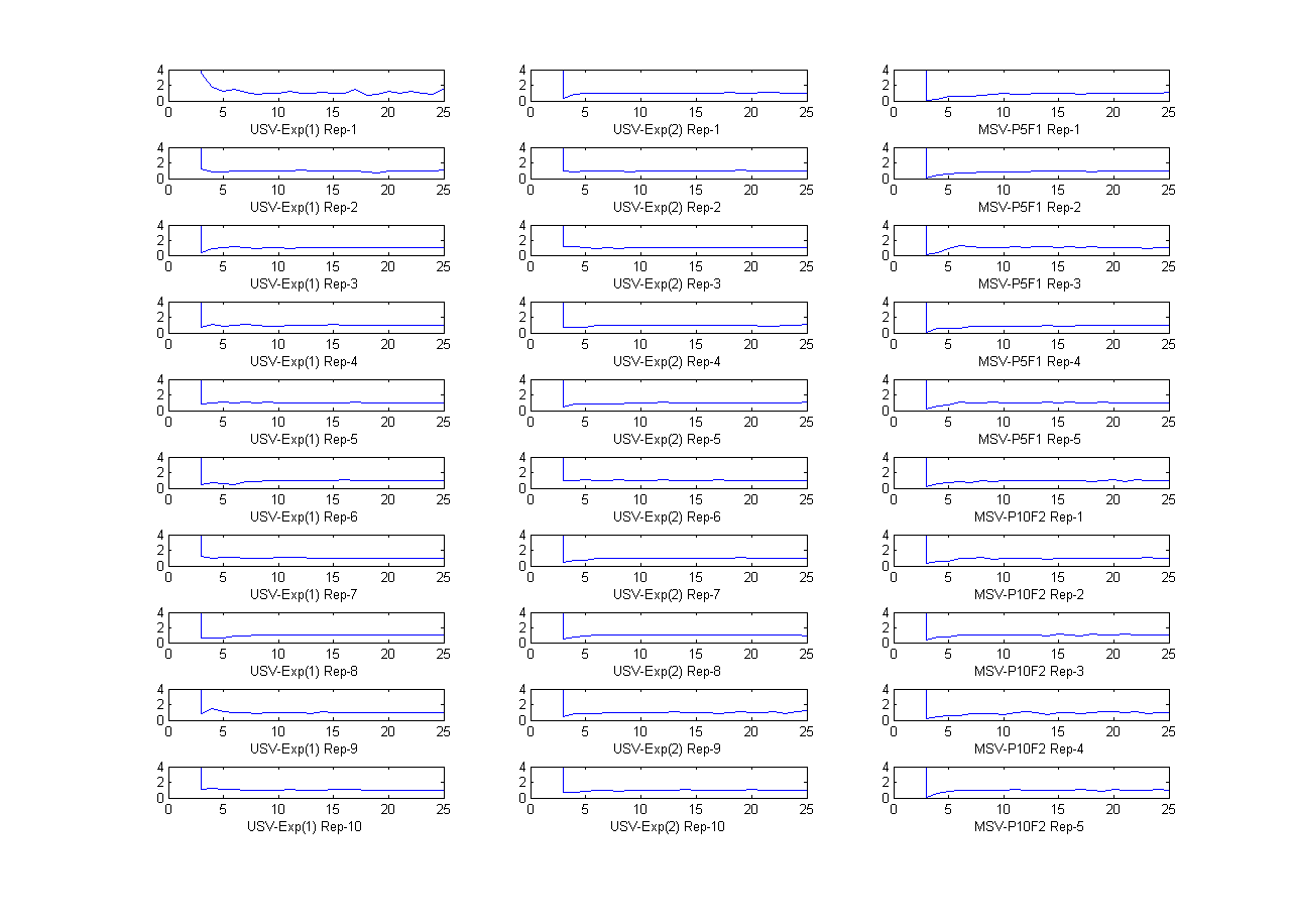
We run 25 iterations for each replication of the Monte Carlo EM method. Figure 1 plots the likelihood ratios against the iterate numbers and shows that likelihood ratios stabilizes before 25 iterations. We therefore take the values of the 25-th iterate as the final estimates. Table 1 shows that the Monte Carlo EM method performs well in terms of its accuracy and is promisingly fast in terms of computing speed with only a few minutes of computing time needed compared with hours using the MCMC methods. Therefore, we expect that by taking the Monte Carlo EM parameter estimates as initial values for the MCMC methods we will obtain a chain that converges quickly. The benefits may not be important in the univariate SV model since both the ‘optimization’ and ‘delayed rejection’ methods converge quickly, but using Monte Carlo EM is worthwhile for the factor MSV model.
5.3 Simulation examples of factor multivariate stochastic volatility models
This section fits the factor MSV model at equation (13) to two simulated datasets using 5 replicates for each dataset. The first dataset which we call ‘P5-K1’ has =5 and =1 and the second dataset which we call ‘P10-K2’ has =10 and =2. Both datasets have 500 observations. The three computational methods (with one-step iteration in the first stage for ‘delayed rejection’) discussed in section 3 are used to estimate the model. The true parameter values are for and for . Table 2 gives the elements in the loading matrices .
The prior specification for both datasets is , for and with the dimensional identity matrix.
For model ‘P5-K1’, we use a one block strategy to sample from for both MCMC methods. For the higher dimensional ‘P10-K2’ model, we use a one block strategy for the ‘optimization’ MCMC method but use a sub-block strategy for the ‘delayed rejection’ MCMC method, with 8 parameters in each sub-block, where the last sub-block contains the remaining parameters if is not a multiple of 8. All the MCMC simulation estimates are again computed using the last 5,000 draws after discarding the first 1,000 burn-in iterations, and is set as 100 after 10 burn-in iterations for Monte Carlo EM. For the Monte Carlo EM method, similar results were obtained for longer burn-in periods and larger values of .
Table 3 summarizes the estimation results for the ‘P5-K1’ model. The estimates from the two MCMC methods agree for almost all the unknown parameters and are also very close to the true parameter values. The inefficiency factor scores are similar for but not for , where the inefficiency of the ‘optimization’ method (7.02) is less than half of the value for the ‘delayed rejection’ method (14.53). However, due to the faster sampling speed of the ‘delayed rejection’ method, the ‘optimization’ method has higher equivalence factor scores than ‘delayed rejection’, with the highest value being 48.71 for compared with the corresponding value of 20.37 using ‘delayed rejection’ (this is almost 2.4 times higher). The parameter estimates from Monte Carlo EM for are consistent with those obtained by MCMC, but a little lower than the MCMC estimates for . Figure 1 plots the likelihood ratios (see equation (11)) vs iteration number for the ‘P5-K1’ model for all the replicates. The plots suggest that the Monte Carlo EM iterates have converged. From Table 3, the Monte Carlo EM method took 6 minutes compared with the 5.1 hours for the ‘optimization’ MCMC method.
Table 4 summarizes the estimation results of the ‘P10-K2’ model. The parameter estimates of the two MCMC methods are again close to the true parameter values. The inefficiency factors are similar for both MCMC methods, but the ‘delayed rejection’ method has lower equivalence factor scores (by a factor of 5) than the ‘optimization’ method because it is five times faster. The acceptance ratios for are almost the same for both MCMC methods. We note that the parameter does not have an acceptance ratio since it is sampled jointly with the latent state from its exact conditional density. However, we observe a significant decrease for the acceptance ratio from 0.87 to 0.66 in the ‘optimization’ method when a one block strategy is used for both simulation cases. Similar results (that are not reported in the article but that are available from the authors) are found for ‘delayed rejection’ method, with a decrease from 0.77 to 0.32 for the first stage acceptance ratio if a one block strategy is used in both examples. Tables 3 and 4 show that for the ‘delayed rejection’ method where a one-block approach is used in the ‘P5-K1’ case but several sub-blocks are used in the ‘P10-K2’ case, there is a small decrease, e.g., from 0.77 to 0.72 in the first stage acceptance ratio, but the acceptance ratio is even higher than the value of 0.66 for the ‘optimization’ method where one block is used in both cases. The benefit of the sub-block strategy in sampling high dimensional is clear in this example.
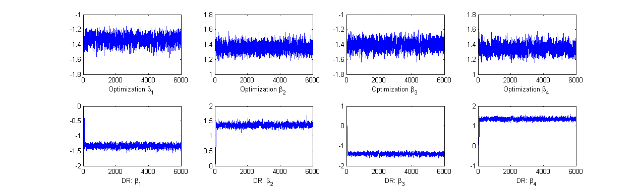
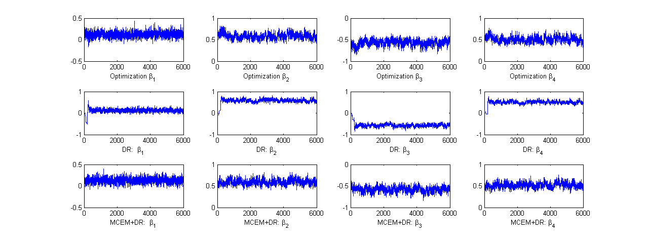
Table 4 also shows that the estimates from the Monte Carlo EM method are similar to those obtained by both MCMC methods for most of the parameters. Figure 1 plots the likelihood ratios vs iteration number for the ‘P10-K2’ model for all the replicates. The figure suggests that the Monte Carlo EM iterations have converged. Figure 2 plots the iterates of the first four elements of for one replicate of ‘P5-K1’ example. Both MCMC methods seem to converge quickly, with the ‘optimization’ method converging almost immediately and the ‘delayed rejection’ method also converging in less than 100 iterations. Figure 3 is a similar plot for the ‘P10-K2’ example. In general, the ‘optimization’ method converges faster than the ‘delayed rejection’ method which takes around 250 iterations to converge. We did not plot the iterates for , since they generally mix very well even in the higher dimensional ‘P10-K2’ example. Figure 3 also plots the iterates when we set the parameter estimates from the Monte Carlo EM method as initial values for the ‘delayed rejection’ method. In this case the chain converges almost immediately. In results for the ‘P10-F2’ example that are not reported in the article, where a one-block strategy for sampling is used for ‘delayed rejection’, it sometimes takes more than 1,000 iterations to obtain convergence which demonstrates the benefits of the sub-block strategy.
The results suggest that the estimates from the Monte Carlo EM method can be used effectively as starting values for the MCMC methods because Monte Carlo EM is much faster than either of the MCMC methods.
5.4 Determining the number of factors
The ‘delayed rejection’ method is applied to fit the two factor MSV simulation examples with factors and evaluate their marginal likelihoods. We use the Gaussian copula approximation method discussed in section 4 to evaluate the posterior ordinate using one ‘Reduced MCMC’ simulation. A similar simulated example in Nott et al. (2009) shows that the posterior ordinate from a Gaussian copula approximation does not change too much for different numbers of sub-block strategies. More importantly, it agrees with the evaluation from the benchmark joint kernel smoothing method using the many sub-blocks strategy in Chib et al. (2006). Therefore, we adopt a one block strategy by only running one ‘Reduced MCMC’ simulation. We run 5,000 iterations in sampling from , and 10,000 particles for and 20,000 particles for in the auxiliary particle filter used to calculate the likelihood.
Table 5 reports the marginal likelihood evaluation results for two simulated examples using 5 replicates. The true number of factors in the ‘P5-K1’ and the ‘P10-K2’ cases are 1 and 2 respectively. The marginal likelihoods suggest one (two) factors for the first (second) examples for all 5 replicates. We did not evaluate the marginal likelihood as in Chib et al. (2006) because it is very slow due to the multiple sub-blocks needed when applying kernel density estimation, with the ‘optimization’ method used for each ‘Reduced MCMC’ sub-block (for evidence see Nott et al. (2009)). However, we believe that based on the results of Nott et al. (2009), ‘delayed rejection’ combined with the copula-based approximation method gives similar results to those of Chib et al. (2006), but is more practical in terms of computational load.
5.5 Faster computing speed
The computational burden for the factor MSV model usually becomes heavier as the dimension increases. However, given and , the model can be decomposed into several independent univariate SV models, so that parallel computing can be used in following areas.
-
I.
Sampling and for univariate SV equations in both MCMC based methods. This can be applied in both the estimation stage and later in the ‘Reduced MCMC’ needed to compute the marginal likelihood.
-
II.
Calculating the gradient corresponding to in the factor MSV model, which is needed for all three methods discussed in section 3.
-
III.
Sampling and for , and evaluating the complete log likelihood within each Monte Carlo simulation for the Monte Carlo EM method.
-
IV.
Calculating the importance weights in the auxiliary particle filter, which can be applied twice since the original auxiliary particle filter needs two re-sampling steps.
5.6 Computing details
All the algorithms in the article are coded in the Matlab M-language running on a PC with Intel®Core 2 Quad CPU (3.0 GHz) under the Matlab®2009a framework with the job assigned to 4 local workers. We believe that the algorithms can be speeded up if coded in C, as in Chib et al. (2006).
6 Real data application
The factor MSV model is now fitted to a real dataset containing 18 international stock indices that cover three major regions: America, Europe and Asian Pacific and both developed and emerging markets. Specifically, they are USA, Canada, Mexico, and Chile in America; UK, Germany, France, Switzerland, Spain, Italy, and Norway in Europe; and Japan, Hong Kong, Australia, New Zealand, Malaysia, Singapore, and Indonesia in Asia-Pacific. We use weekly continuously compounded returns (Wednesday to Wednesday) in nominal local currency from January 10th, 1990 to December 27th, 2006, giving a total of 886 weekly observations. The dataset is obtained from DataStream Morgan Stanley Capital International (MSCI) indices.
The ‘delayed rejection’ method with one iteration in the first stage is applied to estimate the model, using sub-blocks with 8 parameters in each sub-block, to sample from . We use marginal likelihood estimated using a Gaussian copula to select the number of factors, with two sub-blocks used to calculate the ordinate . Table 6 shows the log marginal likelihoods for factors and suggests that the four factor model is the best with the Bayes factors of the 4-factor model compared with the other models all greater than 100, providing strong evidence according to Jeffrey’s scale. We do not list the parameter estimates due to space considerations, but the estimation results show good inefficiency levels: e.g. for the estimation of the 4-factor model we have average inefficiency factor scores of , and , and acceptance ratios and in the first stage.
7 Other Applications
The ‘optimization’ method discussed in Chib and Greenberg (1995) is a powerful approach for MCMC simulation when it is necessary to form a Metropolis-Hastings proposal, either as a single block approach or using multiple sub-blocks. However, it can be quite slow. The ‘delayed rejection’ method discussed in our article can in principle be applied instead. This section discusses several such applications.
7.1 GARCH model
This section applies the ‘delayed rejection’ method to the GARCH volatility model developed by Engle (1982) and generalized by Bollerslev (1986). We first consider the univariate GARCH model which forms the basic building block of the factor multivariate GARCH model discussed in section 7.1.2.
7.1.1 Univariate model
The popular univariate Gaussian-GARCH(1,1) model is
| (22) | ||||
Maximum likelihood estimation (MLE) is a convenient tool to estimate this model, but it may have trouble in more sophisticated GARCH type models such as the factor Multivariate-GARCH (factor-MGARCH) model. Asai (2005) surveys work on Bayesian inference for the univariate GARCH model and compares several existing estimation methods.
We use two simulated examples to compare the performance of the ‘delayed rejection’ method to the ‘Griddy Gibbs’ method (e.g. Bauwens and Lubrano, 1998) the ‘optimization’ method, and to the MLE. Each example uses 1500 observations and 10 replications. The true parameters are for example 1 and for example 2. The volatility persistence parameter is moderate for example 1 and high for example 2.
The priors used for the Bayesian methods are
where is the unconditional variance of . For the ‘Griddy-Gibbs’ method we follow Bauwens and Lubrano (1998), and use 33 grid points with parameter ranges:
.
Table 7 reports the estimation results for the two simulated examples. The parameter estimates are quite accurate for the‘optimization’ and ‘delayed rejection’ and the MLE methods, but not for the ‘Griddy-Gibbs’ method, whose parameter estimates are far from the true values, especially in the second example where the volatility persistence parameter is high. One reason for the poor performance of ‘Griddy-Gibbs’ could be that the range of is too wide in this case, and as suggested in Bauwens and Lubrano (1998), we may further restrict its range while allowing most of the posterior density to fit within this range.
The two block sampling MCMC methods (‘optimization’ and ‘delayed rejection’) usually have lower inefficiency factor scores than the single Gibbs based method, and the ‘delayed rejection’ method compares favourably with the ‘optimization’ method in terms of both inefficiency factors and equivalence factor scores.
7.1.2 Factor-MGARCH model
Although maximum likelihood estimation is much faster than Bayesian methods in the univariate case, Bayesian methods become more attractive for estimating factor multivariate GARCH (factor-MGARCH) models because it is much more difficult to apply the maximum likelihood estimation in this case. See, for example, the discussion in Harvey et al. (1992) who need to make approximation in order to calculate the likelihood of a closely related model. Under suitable assumptions on the factor MGARCH model, parts of the computation can be decomposed into working with several independent univariate GARCH models and the ‘delayed rejection’ can be used to sample both the loading matrix and the parameters in each univariate GARCH model.
7.2 Heavy tailed models
Chib et al. (2006) consider an factor MSV model with Student-t distributions for the idiosyncratic shocks, with for in equation (13), where is the degrees of freedom parameter in the Student-t distribution.
In a Bayesian framework, the Student-t error terms can be expressed in a conditionally normal form so that we can use ‘delayed rejection’ or the simpler ‘-step iteration’ method to build the proposal density in sampling the degrees of freedom parameters, instead of building the proposal densities using the ‘optimization’ method. Similar ideas can be applied in the t-GARCH model with heavy tails.
8 Conclusions
Factor MSV models provide a parsimonious representation of a dynamic multivariate system when the time varying variances and covariances of the time series can be represented by a small number of fundamental factors. Factor MSV models can be used in many financial and economic application such as portfolio allocation, asset pricing, and risk management. MCMC methods are the main tool for estimating the parameters of factor MSV models and determining the number of factors in these models. In particular, the ‘optimization’ method is widely used in the literature to estimate the parameters of stochastic volatility models. Its main shortcoming is its computational expense, because numerical optimization is required to build Metropolis-Hastings proposals in each MCMC iteration. The computational cost is especially heavy for high dimensional models containing many parameters. Evaluating marginal likelihoods to determine the number of factors is even more computationally expensive than model estimation because it may require several reduced MCMC runs for each marginal likelihood evaluation. We propose an alternative MCMC estimation method which is based on ‘delayed rejection’ that is substantially faster than the ‘optimization’ method and is more efficient when measured in terms of equivalence factors. We also propose a fast EM based approximation method for factor MSV models which can be used either on its own or to provide initial parameter estimates to increase the speed of convergence of MCMC methods. We also note that we do not have a good way to determine the number of factors using the Monte Carlo EM approach, whereas the Bayesian approach can use marginal likelihood. Our article also simplifies the marginal likelihood calculation for determining the number of latent factors in the factor MSV model by using Gaussian copula approximations to the marginal ordinates instead of using kernel density estimates. We also show how that our approach also applies in GARCH-type models and compares favorably with existing MCMC estimation methods. The MCMC estimation methods and the fast EM based approximation method proposed in our article reduce the computational cost of estimating factor MSV models considerably, which is important for certain real-time applications in financial markets.
References
- Aguilar and West (2000) Aguilar, O. and West, M. (2000), “Bayesian dynamic factor models and portfolio allocation,” Journal of Business and Economic Statistics, 18, 338–357.
- Anderson and Moore (1979) Anderson, B. and Moore, J. B. (1979), Optimal Filtering, Englewood Cliffs, New Jersey: Prentice Hall.
- Asai (2005) Asai, M. (2005), “Comparison of MCMC methods for estimating GARCH models,” Journal of the Japan Statistical Society, 36, 199–212.
- Bauwens and Lubrano (1998) Bauwens, L. and Lubrano, M. (1998), “Bayesian inference on GARCH models using the Gibbs sampler,” Econometrics Journal, 31, C23–C46.
- Bollerslev (1986) Bollerslev, T. (1986), “Generalized Autoregressive Conditional Heteroskedasticity,” Journal of Econometrics, 31, 307–327.
- Carter and Kohn (1994) Carter, C. and Kohn, R. (1994), “On Gibbs sampling for state space models,” Biometrika, 81, 541–553.
- Carter and Kohn (1997) — (1997), “Semiparametric Bayesian inference for time series with mixed spectra,” Journal of the Royal Statistical Society, Series B, 59, 255–268.
- Chib (1995) Chib, S. (1995), “Marginal likelihood from the Gibbs output,” Journal of the American Statistical Association, 90, 1313–21.
- Chib and Greenberg (1995) Chib, S. and Greenberg, E. (1995), “Understanding the Metropolis-Hastings algorithm,” The American Statistician, 49, 327–35.
- Chib et al. (2002) Chib, S., Nardari, F., and Shephard, N. (2002), “Markov chain Monte Carlo methods for generalized stochastic volatility models,” Journal of Econometrics, 108, 281–316.
- Chib et al. (2006) — (2006), “Analysis of high dimensional multivariate stochastic volatility models,” Journal of Econometrics, 134, 341–371.
- de Jong and Shephard (1995) de Jong, P. and Shephard, N. (1995), “The simulation smoother for time series models,” Biometrika, 82, 339–350.
- Engle (1982) Engle, R. F. (1982), “Autoregressive conditional Heteroskedasticity with estimates of the variance of United Kingdom inflation,” Econometrica,, 50, 987–1007.
- Fruwirth-Schnatter (1994) Fruwirth-Schnatter, S. (1994), “Data augmentation and dynamic linear models,” Journal of time series analysis, 15, 183–202.
- Gamerman (1997) Gamerman, D. (1997), “Sampling from the posterior distribution in generalized linear mixed models,” Statistics and Computing, 7, 57–68.
- Green and Mira (2001) Green, P. and Mira, A. (2001), “Delayed Rejection in Reversible Jump Metropolis-Hastings,” Biometrika, 88, 1035–1053.
- Haario et al. (2005) Haario, H., Saksman, E., and Tamminen, J. (2005), “Componentwise adaptation of high dimensional MCMC,” CSDA, 20, 265–274.
- Han (2006) Han, Y. (2006), “Asset Allocation with a High Dimensional Latent Factor Stochastic Volatility Model,” Review of Financial Studies, 19, 237–271.
- Harvey et al. (1992) Harvey, A. C., Ruiz, E., and Sentana, E. (1992), “Unobserved component time series models with ARCH disturbance,” Journal of Econometrics, 52, 129–157.
- Harvey et al. (1994) Harvey, A. C., Ruiz, E., and Shephard, N. (1994), “Multivariate stochastic variance models,” Review of Economic Studies, 61, 247–264.
- Jacquier et al. (1994) Jacquier, E., Polson, N., and Rossi, P. E. (1994), “Bayesian analysis of stochastic volatility models (with discussion),” Journal of Business and Economic Statistics, 12, 371–417.
- Jungbacker and Koopman (2006) Jungbacker, B. and Koopman, S. J. (2006), “Monte Calo likelihood estimation for three multivariate stochastic volatility models,” Econometric Reviews, 25, 385–408.
- Kim et al. (1998) Kim, S., Shephard, N., and Chib, S. (1998), “Stochastic volatility: likelihood inference and comparison with ARCH models,” Review of Economic Studies, 65, 361–393.
- Liesenfeld and Richard (2006) Liesenfeld, R. and Richard, J.-F. (2006), “Classical and Bayesian analysis of univariate and multivariate stochastic volatility models,” Econometric Reviews, 25, 335–360.
- Lintner (1965) Lintner, J. (1965), “Security prices, risk, and maximal gains from diversification,” Journal of Finance, 20, 587–615.
- McLachlan and Krishnan (2008) McLachlan, G. and Krishnan, T. (2008), The EM algorithm and its extensions, New York: John Wiley and Sons, Inc, 2nd ed.
- Meng and Schilling (1996) Meng, X. and Schilling, S. (1996), “Fitting Full-Information Item Factor Models and an Empirical Investigation of Bridge Sampling,” Journal of the American Statistical Association, 91, 1254–1267.
- Mira (1999) Mira, A. (1999), “Ordering, Slicing and Splitting Monto Carlo Markov Chains,” Ph.D. thesis, University of Minnesota.
- Mira (2001) — (2001), “On Metropolis-Hastings algorithms with delayed rejection,” Metron, LIX, 231–241.
- Nardari and Scruggs (2006) Nardari, F. and Scruggs, J. T. (2006), “Bayesian analysis of linear factor models with latent factors, multivariate stochastic volatility, and APT pricing restrictions,” Journal of Financial and Quantitative Analysis, forthcoming.
- Nott et al. (2009) Nott, D., Kohn, R., Xu, W., and Fielding, M. (2009), “Approximating the marginal likelihood using copula,” Working paper.
- Omori et al. (2007) Omori, Y., Chib, S., Shephard, N., and Nakajima, J. (2007), “Stochastic volatility with leverage: Fast and Efficient likelihood inference,” Journal of Econometrics, 140, 425–449.
- Pitt and Shephard (1999) Pitt, M. and Shephard, N. (1999), “Filtering via simulation: auxiliary particle filter,” Journal of the American Statistical Association, 94, 590–599.
- Roberts and Rosenthal (2009) Roberts, G. O. and Rosenthal, J. S. (2009), “Examples of adaptive MCMC,” "Journal of Computational and Graphical Statistics", 18, 349–367.
- Ross (1976) Ross, S. (1976), “The arbitrage theory of capital asset pricing,” Journal of Finance, 13, 341–360.
- Sharpe (1964) Sharpe, W. (1964), “Capital asset prices: a theory of market equilibrium under conditions of risk,” Journal of Finance, 19, 425–442.
- Shephard (1993) Shephard, N. (1993), “Fitting nonlinear time-series models withh applications to stochastic variance models,” Journal of Applied Econometrics, 8, S135–S152.
- Terrell (1990) Terrell, G. R. (1990), “The maximum smoothing principle in density estimation,” Journal of the American Statistical Association, 85, 470–477.
- Villani et al. (2009) Villani, M., Kohn, R., and Giordani, P. (2009), “Regression density estimation using smooth adaptive Gaussian mixtures,” Journal of Econometrics, forthcoming.
- Wei and Tanner (1990) Wei, G. and Tanner, M. (1990), “A Monte Carlo implementation of the EM algorithm and the poor man’s data augmentation algorithms,” Journal of the American Statistical Association, 85, 699–704.
| Sample Size T=500 | Sample Size T=1,500 | ||||||||||||
|---|---|---|---|---|---|---|---|---|---|---|---|---|---|
| Mean | Stdev | Ineff | Equiv | Acr | Time | Mean | Stdev | Ineff | Equiv | Acr | Time | ||
| 0.469 | 0.143 | 2.35 | 2.40 | 0.37 | 1.7(h) | 0.993 | 0.088 | 2.15 | 7.78 | 0.75 | 6.0(h) | ||
| Optimization- | 0.890 | 0.069 | 14.04 | 13.78 | 0.946 | 0.022 | 5.13 | 18.60 | |||||
| MCMC- | 0.117 | 0.035 | 8.18 | 8.33 | 0.130 | 0.028 | 6.12 | 22.19 | |||||
| k-step | 0.471 | 0.143 | 2.33 | 1.05 | 0.33 | 0.8(h) | 0.994 | 0.088 | 2.14 | 3.02 | 0.67 | 2.4(h) | |
| Iteration- | 0.897 | 0.066 | 15.77 | 7.15 | 0.947 | 0.021 | 7.37 | 10.41 | |||||
| MCMC- | 0.113 | 0.034 | 10.31 | 4.67 | 0.129 | 0.027 | 8.60 | 12.13 | |||||
| Delayed- | 0.469 | 0.159 | 2.07 | 1.12 | 0.32 | 0.9(h) | 0.993 | 0.088 | 2.10 | 3.23 | 0.67 | 2.6(h) | |
| Rejection- | 0.896 | 0.066 | 12.09 | 6.54 | 0.15 | 0.946 | 0.022 | 6.60 | 10.14 | 0.06 | |||
| MCMC | 0.115 | 0.035 | 8.08 | 4.34 | 0.130 | 0.028 | 8.00 | 12.27 | |||||
| Monte | 0.454 | 0.061 | 1.4(m) | 0.991 | 0.066 | 13.1(m) | |||||||
| Carlo- | 0.892 | 0.062 | 0.949 | 0.011 | |||||||||
| EM | 0.115 | 0.010 | 0.121 | 0.007 | |||||||||
| P5-K1: Factor-Loadings | -1.5 | 1.5 | -1.5 | 1.5 | |||||||
| 0 | 0.5 | -0.5 | 0.5 | -0.5 | 0.5 | -0.5 | 0.5 | -0.5 | |||
| P10-K2: Factor-Loadings | 0.5 | -0.5 | 0.5 | -0.5 | 0.5 | -0.5 | 0.5 | -0.5 |
| Panel A: Optimization-MCMC Method | ||||||||||
|---|---|---|---|---|---|---|---|---|---|---|
| Ineff | Equiv | Acr | Time | |||||||
| 0.555 | 0.884 | 0.121 | 1.000 | 3.44 | 10.47 | |||||
| 0.512 | 0.911 | 0.113 | -1.493 | 15.99 | 48.71 | Stage(1) | 0.42 | 5.1(h) | ||
| 0.426 | 0.902 | 0.109 | 1.480 | 9.01 | 27.39 | |||||
| 0.508 | 0.920 | 0.117 | -1.506 | 7.02 | 21.40 | |||||
| 0.524 | 0.906 | 0.126 | 1.475 | Stage(1) | 0.87 | |||||
| 1.102 | 0.968 | 0.123 | ||||||||
| Panel B: Delayed-Rejection: Iteration+Adaptive-MCMC Method | ||||||||||
| 0.556 | 0.896 | 0.117 | 1.000 | 4.67 | 6.50 | |||||
| 0.513 | 0.925 | 0.110 | -1.494 | 14.68 | 20.37 | Stage(1) | 0.38 | 2.3(h) | ||
| 0.429 | 0.915 | 0.106 | 1.482 | 9.92 | 13.81 | Stage(2) | 0.11 | |||
| 0.505 | 0.929 | 0.115 | -1.503 | 14.53 | 19.86 | |||||
| 0.521 | 0.912 | 0.126 | 1.473 | Stage(1) | 0.77 | |||||
| 1.108 | 0.972 | 0.121 | Stage(2) | 0.01 | ||||||
| Panel C: Monte Carlo EM Method | ||||||||||
| 0.539 | 0.881 | 0.099 | 1.000 | 5.9(m) | ||||||
| 0.495 | 0.891 | 0.098 | -1.450 | |||||||
| 0.418 | 0.878 | 0.096 | 1.435 | |||||||
| 0.472 | 0.901 | 0.099 | -1.463 | |||||||
| 0.516 | 0.900 | 0.101 | 1.432 | |||||||
| 1.116 | 0.953 | 0.131 | ||||||||
| Panel A Optimization-MCMC Method | |||||||||||
|---|---|---|---|---|---|---|---|---|---|---|---|
| Ineff | Equiv | Acr | Time | ||||||||
| 0.459 | 0.912 | 0.116 | 1.000 | 1.000 | 10.43 | 145.27 | |||||
| 0.436 | 0.922 | 0.125 | 0.003 | 1.000 | 16.30 | 225.61 | Stage(1) | 0.41 | 23.1(h) | ||
| 0.496 | 0.907 | 0.115 | 0.517 | 0.510 | 9.67 | 133.73 | |||||
| 0.573 | 0.892 | 0.110 | -0.526 | -0.515 | 41.74 | 583.17 | |||||
| 0.513 | 0.895 | 0.107 | 0.495 | 0.498 | Stage(1) | 0.66 | |||||
| 0.540 | 0.903 | 0.112 | -0.510 | -0.532 | |||||||
| 0.549 | 0.891 | 0.112 | 0.516 | 0.499 | |||||||
| 0.533 | 0.893 | 0.122 | -0.507 | -0.526 | |||||||
| 0.496 | 0.913 | 0.114 | 0.515 | 0.497 | |||||||
| 0.541 | 0.902 | 0.112 | -0.515 | -0.484 | |||||||
| 1.131 | 0.967 | 0.127 | |||||||||
| 0.956 | 0.957 | 0.134 | |||||||||
| Panel B Delayed-Rejection: Iteration+Adaptive-MCMC Method | |||||||||||
| 0.443 | 0.915 | 0.113 | 1.000 | 0.000 | 9.74 | 31.51 | |||||
| 0.427 | 0.924 | 0.121 | 0.006 | 1.000 | 15.55 | 48.18 | Stage(1) | 0.37 | 4.4(h) | ||
| 0.494 | 0.915 | 0.113 | 0.506 | 0.524 | 10.42 | 33.25 | Stage(2) | 0.11 | |||
| 0.572 | 0.901 | 0.108 | -0.517 | -0.526 | 40.10 | 131.90 | |||||
| 0.513 | 0.905 | 0.103 | 0.488 | 0.506 | Stage(1) | 0.72 | |||||
| 0.539 | 0.910 | 0.109 | -0.499 | -0.545 | Stage(2) | 0.01 | |||||
| 0.553 | 0.906 | 0.111 | 0.508 | 0.509 | |||||||
| 0.534 | 0.899 | 0.122 | -0.496 | -0.538 | |||||||
| 0.500 | 0.921 | 0.111 | 0.508 | 0.506 | |||||||
| 0.545 | 0.910 | 0.108 | -0.505 | -0.496 | |||||||
| 1.153 | 0.970 | 0.125 | |||||||||
| 0.921 | 0.961 | 0.135 | |||||||||
| Panel C Monte Carlo EM Method | |||||||||||
| 0.501 | 0.881 | 0.098 | 1.000 | 0.000 | 8.8(m) | ||||||
| 0.462 | 0.906 | 0.100 | -0.013 | 1.000 | |||||||
| 0.466 | 0.903 | 0.098 | 0.500 | 0.497 | |||||||
| 0.536 | 0.861 | 0.097 | -0.507 | -0.505 | |||||||
| 0.493 | 0.865 | 0.096 | 0.483 | 0.479 | |||||||
| 0.526 | 0.878 | 0.097 | -0.493 | -0.514 | |||||||
| 0.538 | 0.870 | 0.097 | 0.499 | 0.489 | |||||||
| 0.523 | 0.888 | 0.098 | -0.486 | -0.514 | |||||||
| 0.465 | 0.904 | 0.098 | 0.500 | 0.485 | |||||||
| 0.540 | 0.872 | 0.097 | -0.501 | -0.475 | |||||||
| 1.169 | 0.959 | 0.132 | |||||||||
| 0.888 | 0.949 | 0.134 | |||||||||
| Simulation Example of | Simulation Example of | |||||
|---|---|---|---|---|---|---|
| (true) | (true) | |||||
| Replicate-1 | -5,001.85 | -5,012.58 | -5,021.84 | -9,401.90 | -9,393.32 | -9,400.84 |
| Replicate-2 | -4,967.76 | -4,974.77 | -4,983.24 | -9,563.01 | -9,551.47 | -9,558.68 |
| Replicate-3 | -5,042.42 | -5,051.48 | -5,087.78 | -9,475.16 | -9,423.85 | -9,432.00 |
| Replicate-4 | -5,060.63 | -5,069.60 | -5,078.10 | -9,427.84 | -9,407.43 | -9,418.41 |
| Replicate-5 | -4,958.36 | -4,966.16 | -4,978.47 | -9,521.80 | -9,485.47 | -9,494.53 |
| Sample from | |||||
| Log Marginal-Likelihood | -34,097.05 | -33,722.09 | -33,610.93 | -33,554.69 | -33,594.61 |
| Simulation Example 1 | Simulation Example 2 | ||||||||||||
|---|---|---|---|---|---|---|---|---|---|---|---|---|---|
| Mean | Stdev | Ineff | Equiv | Acr | Time | Mean | Stdev | Ineff | Equiv | Acr | Time | ||
| 0.102 | 0.022 | 1.2(s) | 0.107 | 0.058 | 1.4(s) | ||||||||
| MLE | 0.243 | 0.030 | 0.047 | 0.016 | |||||||||
| 0.703 | 0.032 | 0.899 | 0.040 | ||||||||||
| 0.077 | 0.031 | 6.65 | 3.95 | 59.5(m) | 0.227 | 0.119 | 30.12 | 17.60 | 58.4(m) | ||||
| Griddy- | 0.254 | 0.030 | 5.40 | 3.21 | 0.097 | 0.026 | 9.04 | 5.28 | |||||
| Gibbs- | 0.710 | 0.034 | 10.74 | 6.37 | 0.786 | 0.063 | 31.26 | 18.27 | |||||
| 0.095 | 0.017 | 3.17 | 1.30 | 0.58 | 40.6(m) | 0.101 | 0.029 | 5.16 | 2.22 | 0.46 | 41.9(m) | ||
| Optimization- | 0.231 | 0.029 | 8.43 | 4.02 | 0.048 | 0.013 | 5.68 | 2.44 | |||||
| MCMC- | 0.719 | 0.028 | 7.26 | 3.37 | 0.901 | 0.022 | 5.38 | 2.32 | |||||
| Delayed- | 0.095 | 0.017 | 3.49 | 0.49 | 0.55 | 14.0(m) | 0.099 | 0.027 | 5.11 | 0.70 | 0.36 | 13.6(m) | |
| Rejection- | 0.232 | 0.027 | 3.76 | 0.53 | 0.11 | 0.048 | 0.013 | 5.80 | 0.79 | 0.14 | |||
| MCMC | 0.718 | 0.027 | 4.10 | 0.58 | 0.903 | 0.021 | 5.61 | 0.76 | |||||