Rare decays $B\rightarrow M\nu\bar{\nu}$ in the $TC2$ model
and the $LHT$ model

Abstract

In the framework of the topcolor-assisted technicolor ($TC2$) model and the littlest Higgs model with $T$-parity ($LHT$ model), we consider the rare $B$ decays $B\rightarrow M\nu\bar{\nu}$ with $M=\pi,K,\rho,$ or $K^{\ast}$. We find that the contributions of the $TC2$ model to the branching ratios of these decay processes are larger than those for the $LHT$ model. The experimental upper limits for some branching ratios can give severe constraints on the free parameters of the $TC2$ model.

PACS number: 12.60.Cn, 12.60.Fr, 13.20.He

1. Introduction

$B$ physics plays an important role in testing the standard model ($SM$) and $B$ decays are sensitive to new physics beyond the $SM$ [1]. A large number of $B$ mesons is produced in $B$ factories, such as $Belle$ and $BaBar$ experiments. Recently, there has been significant experimental improvement in measurements of the flavor changing neutral current ($FCNC$) processes related to $B$ mesons at $B$ factories and Tevatron. $B$ physics is entering the era of precision measurement, which is not far from possibly revealing new physics. Rare $B$ decays, which are mediated by $FCNCs$, are good places for new physics to enter through exchange of new particles at the loop level or through new interactions at the tree level. Thus, studying rare $B$ decays in some specific new physics models is very interesting and needed.

The rare $B$ decays $B\rightarrow M\nu\bar{\nu}$ with $M=\pi,K,\rho$, or $K^{\ast}$ belong to the theoretically cleanest decays in the field of $FCNC$ processes, due to the absence of photonic penguin contributions and strong suppression of light quark contributions. Since they are significantly suppressed by the loop momentum and off-diagonal Cabibbo-Kobayashi-Maskawa ($CKM$) matrix-elements in the $SM$ and their long-distance contributions are generally subleading, these rare decay processes are considered as excellent probes of new physics beyond the $SM$. This fact has lead to lot of works for studying the contributions of some popular new physics models to the rare decays $B\rightarrow M\nu\bar{\nu}$ in Refs. [2, 3, 4].

In spite of the above theoretical advantages, experimental search of the rare decays $B\rightarrow M\nu\bar{\nu}$ is a hard task. However, with the advent of Super-B facilities [5], the prospects of measuring the branching ratios of the rare decay processes $B\rightarrow M\nu\bar{\nu}$ in the next decade are possible and it seems appropriate to further study these decays in order to motivate more experimental efforts to measure their branching ratios and related observables. So, in this paper, we reconsider these rare decays processes in the context of the topcolor-assisted technicolor ($TC2$) model [6] and the littlest Higgs model [7, 8] with $T$ parity (called $LHT$ model) [9]. Our numerical results show that these two kinds of popular new physics models can indeed give significant contributions to these rare $B$ decay processes and the current experimental limits for some of these processes can put severe constraints on the free parameters of the $TC2$ model. Furthermore, in the context of the $TC2$ model, we consider that the contributions of the nonuniversal gauge boson $Z^{\prime}$ to the quark level transition processes $b\to sl^{+}l^{-}$ are correlated with those for the quark level transition processes $b\to s\nu\bar{\nu}$ and recalculate the contributions of $Z^{\prime}$ to the rare decay processes $B\rightarrow M\nu\bar{\nu}$. We also compare our numerical results with those obtained in Ref. [4].

In the rest of this paper, we will give our results in detail. After briefly summarizing the essential features of the $TC2$ model, we calculate the contributions of the new particles predicted by this model to the rare $B$ decays $B\rightarrow M\nu\bar{\nu}$ with $M=\pi,K,\rho,K^{\ast}$ in section 2. To compare our results obtained in the context of the $TC2$ model with those of the $LHT$ model, the branching ratios of these decay processes contributed by the $LHT$ model are estimated in section 3 by using the results of Refs. [10, 11]. Our conclusions are given in section 4.

2. The $TC2$ model and the rare decays $B\rightarrow M\nu\bar{\nu}$

In the $TC2$ model [6], topcolor interactions, which are not flavor-universal and mainly couple to the third generation fermions, generally generate small contributions to electroweak symmetry breaking ($EWSB$) and give rise to the main part of the top quark mass. Thus, the nonuniversal gauge boson $Z^{\prime}$ has large Yukawa couplings to the third generation fermions. Such features can result in large tree level flavor changing ($FC$) couplings of the nonuniversal gauge boson $Z^{\prime}$ to ordinary fermions when one writes the interaction in the fermion mass eigen-basis.

The flavor diagonal ($FD$) couplings of the nonuniversal gauge boson $Z^{\prime}$ to ordinary fermions, which are related to our calculation, can be written as [6, 12, 13]:

$$\mathcal{L}^{FD}_{Z^{\prime}} = -\sqrt{4\pi K_{1}}\left\{Z^{\prime}_{\mu}\left[\frac{1}{6}\bar{t}_{L}\gamma^{\mu}t_{L}+\frac{1}{6}\bar{b}_{L}\gamma^{\mu}b_{L}+\frac{2}{3}\bar{t}_{R}\gamma^{\mu}t_{R}-\frac{1}{3}\bar{b}_{R}\gamma^{\mu}b_{R}-\frac{1}{2}\bar{\nu}_{\tau L}\gamma^{\mu}\nu_{\tau L}\right]\right.$$ (1)

$$-\left.\tan^{2}\theta^{\prime}Z^{\prime}_{\mu}\left[\frac{1}{6}\bar{s}_{L}\gamma^{\mu}s_{L}-\frac{1}{3}\bar{s}_{R}\gamma^{\mu}s_{R}+\frac{1}{6}\bar{d}_{L}\gamma^{\mu}d_{L}-\frac{1}{3}\bar{d}_{R}\gamma^{\mu}d_{R}-\frac{1}{2}\bar{\nu}_{\mu L}\gamma^{\mu}\nu_{\mu L}\right.\right.$$

$$-\left.\left.\frac{1}{2}\bar{\nu}_{eL}\gamma^{\mu}\nu_{eL}\right]\right\},$$

where $K_{1}$ is the coupling constant, $\theta^{\prime}$ is the mixing angle with $\tan\theta^{\prime}=\frac{g_{1}}{\sqrt{4\pi K_{1}}}$ , and $g_{1}$ is the ordinary hypercharge gauge coupling constant.

The $FC$ couplings of the nonuniversal gauge boson $Z^{\prime}$ to down-type quarks, i.e. $Z^{\prime}bd_{j}$ with $j=s$ or $d$, can be written as [13]:

$$\mathcal{L}^{FC}_{Z^{\prime}}=-\frac{g_{1}}{2}\cot\theta^{\prime}Z^{\prime\mu}\left\{\frac{1}{3}D^{bb}_{L}D^{bd_{j}\ast}_{L}\bar{d_{j}}_{L}\gamma_{\mu}b_{L}-\frac{2}{3}D^{bb}_{R}D^{bd_{j}\ast}_{R}\bar{d_{j}}_{R}\gamma_{\mu}b_{R}+h.c.\right\},$$ (2)

where $D_{L}$ and $D_{R}$ are matrices which rotate the down-type left- and right- handed quarks from the quark field to mass eigen-basis, respectively.

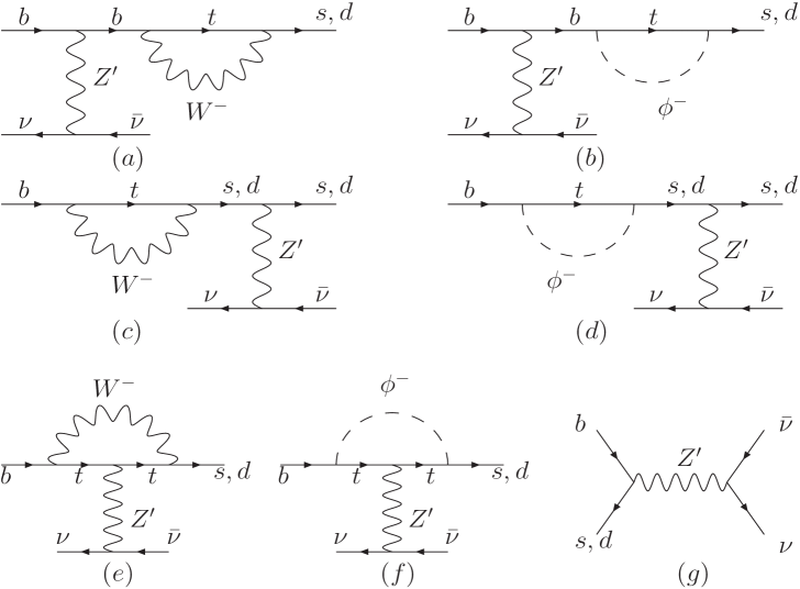
Figure 1: The penguin and tree level diagrams for $Z^{\prime}$ contributing to the rare decay                  processes $b\rightarrow(s,d)\nu\bar{\nu}$ in the $TC2$ model.

The quark level transition $b\rightarrow d_{j}\nu\bar{\nu}$ ($j=s$ or $d$) is responsible for the semi-leptonic decays $B\rightarrow M\nu\bar{\nu}$($M=\pi,K,\rho,K^{\ast}$). From the above discussions, we can see that the nonuniversal gauge boson $Z^{\prime}$ can contribute to the rare decay processes $b\rightarrow(s,d)\nu\bar{\nu}$ at the tree level and the one loop level. The relevant Feynman diagrams are shown in Fig.1. In these diagrams, the Goldstone boson $\phi$ is introduced by the ’t Hooft-Feynman gauge, which can cancel the divergence in self-energy diagrams.

The effective Hamiltonian for the transition $b\rightarrow d_{j}\nu_{i}\bar{\nu_{i}}$ ($j=s,d$ and $i=e,\mu,\tau$) can be written as [14]:

$$\mathcal{H}_{eff}(b\rightarrow d_{j}\nu_{i}\bar{\nu_{i}}) = C^{\nu}_{L}\bar{b}\gamma_{\mu}(1-\gamma_{5})d_{j}\bar{\nu_{i}}\gamma^{\mu}(1-\gamma_{5})\nu_{i}+C^{\nu}_{R}\bar{b}\gamma_{\mu}(1+\gamma_{5})d_{j}\bar{\nu_{i}}\gamma^{\mu}(1-\gamma_{5})\nu_{i}$$ (3)

$$\equiv C^{\nu}_{L}\mathcal{O}_{L}+C^{\nu}_{R}\mathcal{O}_{R}$$

$\mathcal{O}_{L(R)}$ and $C^{\nu}_{L(R)}$ represent the left- (right-) handed operators and the corresponding coefficients, respectively. By the way, these operators and coefficients are defined with opposite signs w.r.t. those in Ref. [4]. In the $SM$, the processes $b\rightarrow d_{j}\nu_{i}\bar{\nu_{i}}$ proceed via $W$ box and $Z$ penguin diagrams, therefore only purely left-handed currents $\bar{b}\gamma_{\mu}(1-\gamma_{5})d_{j}\bar{\nu_{i}}\gamma^{\mu}(1-\gamma_{5})\nu_{i}$ are present. The corresponding left-handed coefficient reads

$$C^{\nu}_{L,SM}=\frac{G_{F}\alpha_{e}}{2\pi\sqrt{2}}V_{td_{j}}V_{tb}^{\ast}\frac{X(x_{t})}{\sin^{2}\theta_{w}},$$ (4)

where $G_{F}$ is the Fermi constant, $\alpha_{e}$ is the fine structure constant, $\theta_{w}$ is the Weinberg angle, and $V_{ij}$ is the $CKM$ matrix element. The $SM$ Inami-Lim function $X(x_{t})$ [15] is dominated by the short distance dynamics associated with top quark exchange. $\mathcal{O}_{R}$ is one new right-handed operator induced by new physics effects with $C^{\nu}_{R}$ only receiving contributions from new physics beyond the $SM$.

It is obvious that the nonuniversal gauge boson $Z^{\prime}$ predicted by the $TC2$ model can give corrections to the coefficient $C^{\nu}_{L,SM}$ via both the penguin and tree level diagrams, while it can give contributions to the coefficient $C^{\nu}_{R}$ only via the tree level diagram. From the Feynman diagrams given in Fig.1, we can obtain the corresponding coefficients in Eq.(3) contributed by $Z^{\prime}$. For $\nu_{i}=\nu_{e}$ and $\nu_{\mu}$, their expression forms can be written as:

$$C^{\nu}_{L} = C^{\nu}_{L,SM}+\frac{\tan^{2}\theta^{\prime}g^{2}}{4M_{Z^{\prime}}}\left[\frac{g_{2}^{2}V^{\ast}_{tb}V_{td_{j}}}{8(4\pi^{2})}X^{TC}(x_{t})-\frac{1}{12}D^{bb^{\ast}}_{L}D^{bd_{j}}_{L}\right],$$ (5)

$$C^{\nu}_{R} = \frac{\tan\theta^{\prime}g^{2}}{24M_{Z^{\prime}}}D^{bb^{\ast}}_{R}D^{bd_{j}}_{R},$$ (6)

$$X^{TC}(x_{t}) = C_{a}(x_{t})+C_{b}(x_{t})+C_{c}(x_{t}).$$ (7)

Here $x_{t}=\frac{m_{t}^{2}}{M_{W}^{2}}$ and $g=\sqrt{4\pi K_{1}}$. Using the method given in Ref. [15], we can calculate the functions $C_{a}(x_{t})$, $C_{b}(x_{t})$ and $C_{c}(x_{t})$ in the framework of the $TC2$ model. $C_{a}(x_{t})$ is obtained from the penguin diagrams Fig.1 $(a)$,$(b)$,$(c)$ and $(d)$, $C_{b}(x_{t})$ is obtained from the penguin diagram Fig.1 $(e)$, $C_{c}(x_{t})$ is obtained from the penguin diagram Fig.1 $(f)$. The third term of the coefficient $C^{\nu}_{L}$ and the coefficient $C^{\nu}_{R}$ are contributed by Fig.1 $(g)$. The detailed expression forms of these functions are listed in Appendix.

From Eq. (2) we can see that, for the processes $b\rightarrow d_{j}\nu_{\tau}\bar{\nu}_{\tau}$, the expression forms of the coefficients $C^{\nu}_{L}$ and $C^{\nu}_{R}$ are similar to those for the processes $b\rightarrow d_{j}\nu_{e}\bar{\nu}_{e}$. However, the factor $\tan^{2}\theta^{\prime}$ should be omitted.

The decay amplitudes of the exclusive semi-leptonic decay processes $B\rightarrow M\nu\bar{\nu}$($M=\pi,K,\rho,K^{\ast}$) can be obtained after evaluating matrix elements of the quark operators given in Eq. (3) between the initial $|B>$ and final $|M>$ states. The hadronic matrix elements for $B\rightarrow P$ decay ($P$ is a pseudoscalar meson, $\pi$ or $K$) can be parameterized in terms of the form factors $f^{P}_{+}(s_{B})$ and $f^{P}_{0}(s_{B})$ as [2, 3, 4, 16]:

$$c_{p}\langle P(p)|\bar{u}\gamma_{\mu}b|B(p_{B})\rangle=f^{P}_{+}(s_{B})(p+p_{B})_{\mu}+[f^{P}_{0}(s_{B})-f^{P}_{+}(s_{B})]\frac{m^{2}_{B}-m^{2}_{P}}{s_{B}}q_{\mu},$$ (8)

where the factor $c_{P}$ accounts for flavor content of particles ($c_{P}$ = $\sqrt{2}$ for $\pi^{0}$ and $c_{P}$ = 1 for $\pi^{-}$, $K^{-}$) and $s_{B}$ = $q^{2}$ ($q$ = $p_{B}-p$ = $p_{\nu}+p_{\bar{\nu}}$). For $B\rightarrow V$ decay ($V$ is a vector mesons $K^{\ast}$ or $\rho$ ), its hadronic matrix elements can be written in terms of five form factors:

$$c_{V}\langle V(p,\varepsilon^{\ast})|\bar{u}\gamma_{\mu}(1-\gamma_{5})b|B(p_{{}_{B}})\rangle =\frac{2V(s_{B})}{m_{B}+m_{V}}\epsilon_{\mu\nu\alpha\beta}\varepsilon^{\ast\nu}p_{{}_{B}}^{\alpha}p^{\beta}$$ (9)

$$-i\left[\varepsilon_{\mu}^{\ast}(m_{B}+m_{V})A_{1}(s_{B})-(p_{{}_{B}}+p)_{\mu}({\varepsilon^{\ast}}\cdot{p_{{}_{B}}})\frac{A_{2}(s_{B})}{m_{B}+m_{V}}\right]$$

$$+iq_{\mu}({\varepsilon^{\ast}}\cdot{p_{{}_{B}}})\frac{2m_{V}}{s_{B}}[A_{3}(s_{B})-A_{0}(s_{B})]$$

with

$$V(s_{B}) = \frac{V(0)}{1-s_{B}^{2}/M^{2}_{p}},\quad\quad M_{p}=5~{}\rm GeV,$$ (10)

$$A_{3}(s_{B}) = \frac{m_{B}+m_{V}}{2m_{V}}A_{1}(s_{B})-\frac{m_{B}-m_{V}}{2m_{V}}A_{2}(s_{B}),$$ (11)

where $c_{V}=\sqrt{2}$ for $\rho^{0}$, $c_{V}=1$ for $\rho^{-}$ and $K^{*-}$.

The form factors $f^{P}_{+}(s_{B})$ and $f^{P}_{0}(s_{B})$ given in Ref. [17] are valid in the full physical range $0\leq s_{B}\leq(1-m_{P})^{2}$. So we will use the form factors given in Ref. [17] to estimate the branching ratio of the decay process $B\to P\nu\bar{\nu}$, which are same as those used in Ref. [4]. While for the form factors $V(s_{B})$, $A_{1}(s_{B})$, and $A_{2}(s_{B})$, we will use those given by Ref. [18], which is same as the form factors (set C) used in Ref. [4]. It has been shown [4] that the differential branching ratio for the decay process $B\to K^{\ast}\nu\bar{\nu}$ is similar for sets A and B, there is a difference of about $25\%$ relative to the results obtained from set C. Certainly, this conclusion also applies to our paper. The detailed expressions of the form factors $f^{P}_{i}$ and $A_{i}$ are listed in Appendix.

The di-neutrino invariant mass distributions for the decay processes $B\to P\nu\bar{\nu}$ and $B\to V\nu\bar{\nu}$ can be written as:

$$\frac{d\mathcal{B}(B\to P\nu_{i^{\prime}}\bar{\nu}_{i})}{ds_{B}} = \left|C^{\nu}_{L}+C^{\nu}_{R}\right|^{2}\frac{\tau_{B}m_{B}^{3}}{2^{5}\pi^{3}c_{P}^{2}}\lambda_{P}^{3/2}(s_{B})\left[f^{P}_{+}(s_{B})\right]^{2},$$ (12)

$$\frac{d\mathcal{B}(B\to V\nu_{i^{\prime}}\bar{\nu}_{i})}{ds_{B}} = \left|C^{\nu}_{L}+C^{\nu}_{R}\right|^{2}\frac{\tau_{B}m_{B}^{3}}{2^{7}\pi^{3}c_{V}^{2}}\lambda_{V}^{1/2}(s_{B})\frac{8s_{B}\lambda_{V}(s_{B})V^{2}(s_{B})}{(1+\sqrt{r_{V}})^{2}}$$ (13)

$$+ \left|C^{\nu}_{L}-C^{\nu}_{R}\right|^{2}\frac{\tau_{B}m_{B}^{3}}{2^{7}\pi^{3}c_{V}^{2}}\lambda_{V}^{1/2}(s_{B})\frac{1}{r_{V}}\left[(1+\sqrt{r_{V}})^{2}(\lambda_{V}(s_{B})+12r_{V}s_{B})A_{1}^{2}(s_{B})\frac{}{}\right.$$

$$+ \left.\frac{\lambda_{V}^{2}(s_{B})A_{2}^{2}(s_{B})}{(1+\sqrt{r_{V}})^{2}}-2\lambda_{V}(s_{B})(1-r_{V}-s_{B})A_{1}(s_{B})A_{2}(s_{B})\right].$$

Here

$$\lambda_{V}(s_{B})=\lambda(1,r_{V},s_{B}/m_{B}^{2})=1+r_{V}^{2}+\frac{s^{2}}{m^{4}_{B}}-2r_{V}-\frac{2s}{m^{2}_{B}}-\frac{2r_{V}s_{V}}{m_{B}^{2}},$$ (14)

where $r_{V}=m^{2}_{V}/m_{B}^{2}$, and $\lambda_{P}$ is similar to $\lambda_{V}$ by changing $V$ to $P$.

$$G_{F}=1.166\times 10^{-5}\;{\rm GeV}^{-2}$$

Table 1: Numerical inputs used in our analysis. Unless explicitly specified, they are                 taken from the Particle Data Group [19].

To obtain numerical results, we need to specify the relevant $SM$ parameters. Most of these input parameters have been shown in Table 1. It is obvious that, except these $SM$ input parameters, the branching ratio $Br(B\rightarrow M\nu\bar{\nu})$ is dependent on the model dependent parameters $M_{Z^{\prime}}$ and $K_{1}$. The lower limits on the mass parameter $M_{Z^{\prime}}$ predicted by the topcolor scenario can be obtained via studying its effects on various observables, which have been precisely measured in the high energy collider experiments [12]. The most severe constraints come from the precision electroweak data, which demand that the $Z^{\prime}$ mass $M_{Z^{\prime}}$ must be larger than $1TeV$ [20]. The vacuum tilting, the constraints from $Z$-pole physics, and $U(1)$ triviality require $K_{1}\leq 1$ [21]. Thus, in our numerical calculation, we will take them as free parameters and assume that they are in the ranges of $1~{}\rm TeV\leq M_{Z^{\prime}}\leq 2~{}\rm TeV$ and $0<K_{1}\leq 1$.

Observable	Exp. Data	SM Predictions	$M_{Z^{\prime}}(\rm GeV)$ =$1100$	$1400$	$1700$	$2000$
$\mathcal{B}(B_{d}^{0}\rightarrow K^{0}\nu\bar{\nu})$	$<160$	$[3.48,6.55]$	$6.41$	$5.55$	$5.26$	$5.15$
			$10.59$	$7.14$	$6.00$	$5.53$
$\mathcal{B}(B_{u}^{+}\rightarrow K^{+}\nu\bar{\nu})$	$<14$	$[3.75,7.04]$	$8.19$	$6.46$	$5.89$	$5.66$
			$16.56$	$9.65$	$7.36$	$6.42$
$\mathcal{B}(B_{d}^{0}\rightarrow\pi^{0}\nu\bar{\nu})$	$<220$	$[0.05,0.12]$	$0.61$	$0.29$	$0.18$	$0.14$
			$2.18$	$0.89$	$0.46$	$0.28$
$\mathcal{B}(B_{u}^{+}\rightarrow\pi^{+}\nu\bar{\nu})$	$<100$	$[0.11,0.25]$	$1.22$	$0.58$	$0.36$	$0.27$
			$4.37$	$1.78$	$0.91$	$0.56$
$\mathcal{B}(B_{d}^{0}\rightarrow K^{\ast 0}\nu\bar{\nu})$	$<120$	$[6.98,15.19]$	$163.09$	$69.02$	$37.73$	$25.00$
			$618.45$	$242.56$	$117.56$	$66.67$
$\mathcal{B}(B_{u}^{+}\rightarrow K^{\ast+}\nu\bar{\nu})$	$<80$	$[7.55,16.35]$	$327.43$	$132.18$	$67.25$	$40.82$
			$1272.62$	$492.41$	$232.94$	$127.31$
$\mathcal{B}(B_{d}^{0}\rightarrow\rho^{\ast 0}\nu\bar{\nu})$	$<440$	$[0.10,0.29]$	$72.42$	$27.73$	$12.86$	$6.81$
			$287.9$	$109.85$	$50.63$	$26.52$
$\mathcal{B}(B_{u}^{+}\rightarrow\rho^{\ast+}\nu\bar{\nu})$	$<150$	$[0.22,0.62]$	$144.84$	$55.47$	$25.74$	$13.64$
			$1377.35$	$525.19$	$241.79$	$126.42$

Table 2: The values (in units of $10^{-6}$ ) of the branching ratios for the semi-leptonic decays                  $B\rightarrow M\nu\bar{\nu}$($M=\pi,K,\rho,K^{\ast}$) for $K_{1}=0.4$ (the first line), $K_{1}=0.8$ (the second line),                  and different values of $M_{Z^{\prime}}$.

The values (in units of $10^{-6}$ ) of the branching ratios for the semi-leptonic decays $B\rightarrow M\nu\bar{\nu}$ ($M=\pi,K,\rho,K^{\ast}$), contributed by the nonuniversal gauge boson $Z^{\prime}$, are displayed in Table 2 for the coupling parameter $K_{1}=0.4$ (the first line of every row) and $0.8$ (the second line of every row). The second and third columns in Table 2 express the corresponding experimental upper limits and the $SM$ prediction values, respectively. From this table, one can see that the nonuniversal gauge boson $Z^{\prime}$ predicted by the $TC2$ model can indeed generate significant contributions to these $FCNC$ decay processes. The values of their branching ratios are sensitive to the free parameters $M_{Z^{\prime}}$ and $K_{1}$. In most of the parameter space, the contributions of $Z^{\prime}$ to the $FCNC$ decay processes $B\to V\nu\bar{\nu}$ are larger than those for the $FCNC$ decay processes $B\to P\nu\bar{\nu}$, which is easily apprehended from Eqs. (12) and (13) and the relevant couplings of the nonuniversal gauge boson $Z^{\prime}$ with quarks given in Eqs. (1) and (2). In wide range of the parameter space, the new gauge boson $Z^{\prime}$ can make the values of the branching ratio $Br(B\to V\nu\bar{\nu})$ exceed the corresponding experimental upper limit.

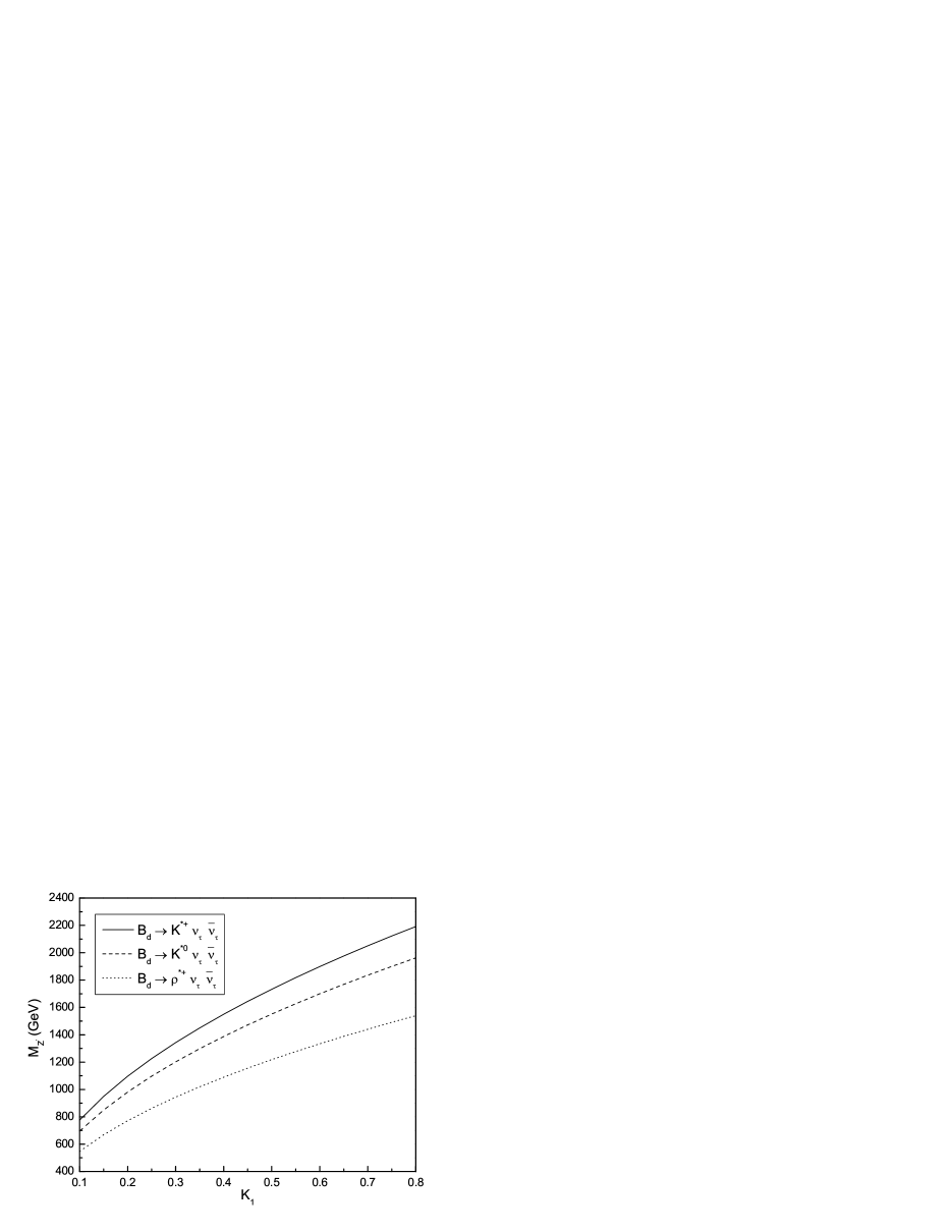
Figure 2: The mass parameter $M_{Z^{\prime}}$ as a function of the coupling parameter $K_{1}$ for                  $Br^{TC2}(B\to V\nu\bar{\nu})=Br^{exp}(B\to V\nu\bar{\nu})$.

To see whether the present experimental upper limit for the branching ratio $Br(B\to V\nu\bar{\nu})$ can give constraints on the free parameters of the $TC2$ model, we let that its value equals to the corresponding experimental upper limit, and plot the mass parameter $M_{Z^{\prime}}$ as a function of the coupling parameter $K_{1}$ in Fig.2, in which the solid line, dotted line, and dashed line denote the $FCNC$ decay processes $B_{u}^{+}\rightarrow K^{\ast+}\nu_{\tau}\bar{\nu}_{\tau}$, $B_{d}^{+}\rightarrow\rho^{\ast+}\nu_{\tau}\bar{\nu}_{\tau}$, and $B_{d}^{0}\rightarrow K^{\ast 0}\nu_{\tau}\bar{\nu}_{\tau}$, respectively. From this figure, we can see that the present experimental upper limits of these $FCNC$ decay processes can indeed give severe constraints on the relevant free parameters. The constraints coming from the $FCNC$ decay process $B_{u}^{+}\rightarrow K^{\ast+}\nu_{\tau}\bar{\nu}_{\tau}$ is the strongest, which demands that if we desire $M_{Z^{\prime}}\leq 2~{}\rm TeV$, there must be $K_{1}\leq 0.65$.

The presence of the physical scalars, the top-pions $\pi_{t}^{0,\pm}$ and the top-Higgs boson $h_{t}^{0}$, in the low energy spectrum is an inevitable feature of the topcolor scenario, regardless of the dynamics responsible for $EWSB$ and other quark masses [12]. These new particles treat the third generation fermions differently from those in the first and second generation fermions and thus can lead to the tree level $FC$ couplings to ordinary fermions. So they can also generate contributions to some $FCNC$ processes.

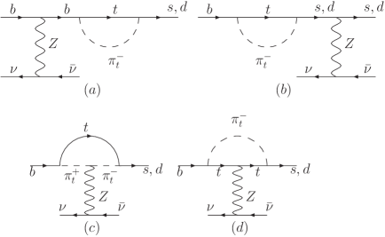
Figure 3: The penguin diagrams for $\pi_{t}^{\pm}$ contributing to the rare decay processes                   $b\rightarrow(s,d)\nu\bar{\nu}$ in the $TC2$ model.

In the context of the $TC2$ model, the couplings of the charged top-pions $\pi_{t}^{\pm}$ to ordinary fermions, which are related to our calculation, can be written as [6, 13, 22]:

$$\frac{m_{t}^{*}}{F_{\pi}}\frac{\sqrt{\nu_{w}^{2}-F_{\pi}^{2}}}{\nu_{w}}\left[\bar{t}_{R}b_{L}\pi_{t}^{+}+\bar{b}_{L}t_{R}\pi_{t}^{-}+K_{UR}^{tc^{*}}K_{DL}^{ss}\bar{t}_{R}s_{L}\pi_{t}^{+}+K_{UR}^{tc}K_{DL}^{ss^{*}}\bar{s}_{L}t_{R}\pi_{t}^{-}\right],$$ (15)

where $m_{t}^{*}=m_{t}(1-\varepsilon)$, $\nu_{w}=\nu/\sqrt{2}=174\rm~{}GeV$, $F_{\pi}\approx 50\rm~{}GeV$ is the top-pion decay constant. $K_{UR}$ and $K_{DL}$ are rotation matrices that diagonalize the up-quark and down-quark mass matrices $M_{U}$ and $M_{D}$, i.e., $K_{UL}^{+}M_{U}K_{UR}=M_{U}^{dia}$ and $K_{DL}^{+}M_{D}K_{DR}=M_{D}^{dia}$, for which the $CKM$ matrix is defined as $V=K_{UL}^{+}K_{DL}$. To yield a realistic form of the $CKM$ matrix $V$, it has been shown that the values of the coupling parameters can be taken as [22]:

$$K_{DL}^{ss}\approx 1,\hskip 28.45274ptK_{UR}^{tc}\leq\sqrt{2\varepsilon-\varepsilon^{2}}.$$ (16)

In numerical estimation, we will take $K_{UR}^{tc}=\sqrt{2\varepsilon-\varepsilon^{2}}$ and assume that the value of the free parameter $\varepsilon$ is in the range of $0.03-0.1$.

The charged top-pions $\pi_{t}^{\pm}$ can contribute to the quark level transition $b\rightarrow d_{j}\nu\bar{\nu}(j=s,d)$ via the penguin diagrams, as shown in Fig.3. However, the $FC$ coupling $\pi_{t}^{\pm}ts$ or $\pi_{t}^{\pm}td$ is suppressed by a factor $K_{UR}^{tc}$ with $\varepsilon$ in the range of $0.03-0.1$. Thus, the contributions of the top-pions $\pi^{\pm}_{t}$ to the rare decay processes $b\rightarrow(s,d)\nu\bar{\nu}$ are much smaller than those of the nonuniversal gauge boson $Z^{\prime}$. Our numerical results show that it indeed is this case. The value of the branching ratio $Br(B\rightarrow M\nu\bar{\nu})$ contributed by the scalars $\pi^{\pm}_{t}$ is smaller than that of $Z^{\prime}$ at least by two orders of magnitude, which is consistent with the conclusion obtained in Ref. [23].

In Ref. [23], we consider the contributions of the $TC2$ model to the branching ratios and asymmetry observables related to the quark level transition $b\to sl^{+}l^{-}$. We find that the contributions of the scalar predicted by the $TC2$ model to the decay process $B\to K\tau^{+}\tau^{-}$ are smaller than those of the nonuniversal gauge boson $Z^{\prime}$ by two orders of magnitude and therefore can be neglected. When the $Z^{\prime}$ mass is in the range of $1000\rm~{}GeV-2000\rm~{}GeV$, the value of $Br(B\to K\tau^{+}\tau^{-})$ is in the range of $7.0\times 10^{-6}-1.7\times 10^{-6}$, which is larger than those for the decay process $B\to Ke^{+}e^{-}$ or $B\to K\mu^{+}\mu^{-}$. This is because of the large coupling of $Z^{\prime}$ to the third generation fermions. If we assume that the experimental constraint for the branching ratio of the rare decay process $B\to Kl^{+}l^{-}$ provided by BaBar and Belle experiments is $Br(B\rightarrow Kl^{+}l^{-})=(1.6\pm 0.5)\times 10^{-6}$ [24], then we can easily obtain the constraints on the free parameters $K_{1}$ and $M_{Z^{\prime}}$. For example, for $K_{1}=0.4$, there must be $1290GeV\leq M_{Z^{\prime}}\leq 1787GeV$. In the case of considering these constraints on the relevant free parameters, the contributions of the nonuniversal gauge boson $Z^{\prime}$ to the rare decays $B\rightarrow M\nu\bar{\nu}$ would be reduced. For instance, for $K_{1}=0.4$ and $1290GeV\leq M_{Z^{\prime}}\leq 1787GeV$, there are $2.14\times 10^{-5}\leq Br(B_{d}^{+}\rightarrow\rho^{+}\nu_{\tau}\bar{\nu}_{\tau})\leq 7.64\times 10^{-5}$, $5.70\times 10^{-5}\leq Br(B_{u}^{+}\rightarrow K^{\ast+}\nu_{\tau}\bar{\nu}_{\tau})\leq 1.82\times 10^{-4}$, and $3.31\times 10^{-5}\leq Br(B_{d}^{0}\rightarrow K^{\ast 0}\nu_{\tau}\bar{\nu}_{\tau})\leq 9.11\times 10^{-5}$. It is also possible that the value of the branching ratio $B\rightarrow M\nu\bar{\nu}$ is larger than the corresponding value predicted by the $SM$. Thus, the contributions of the nonuniversal gauge boson $Z^{\prime}$ to the quark level transition processes $b\to sl^{+}l^{-}$ are correlated with those for the quark level transition processes $b\to s\nu\bar{\nu}$. However, even if the experimental measurement value of the branching ratio $Br(B\to X_{s}l^{+}l^{-})$ gives severe constraints on the relevant free parameters, it is still possible to largely enhance the branching ratios related to the quark level transition processes $b\to s\nu\bar{\nu}$ in the $TC2$ model. These conclusions are consistent with those given in Ref. [4] for a general $Z^{\prime}$ model.

3. The $LHT$ model and the rare decays $B\rightarrow M\nu\bar{\nu}$

Little Higgs theory [8] was proposed as an alternative solution to the hierarchy problem of the $SM$, which provides a possible kind of the $EWSB$ mechanism accomplished by a naturally light Higgs boson. In matter content, the littlest Higgs ($LH$) model [7] is the most economical little Higgs model discussed in the literature, which has almost all of the essential feature of the little Higgs models. In order to make this model consistent with electroweak precision tests and simultaneously having the new particles of this model in the reach of the $LHC$, a discrete symmetry, T-parity, has been introduced, which forms the $LHT$ model [9]. This new physics model is one of the attractive little Higgs models. In which, all the $SM$ particles are even and among the new particles only a heavy $2/3$ charged T quark belongs to the even sector.

A consistent implementation of T-parity also requires the introduction of mirror fermions – one for each quark and lepton species [9, 25]. The masses of the T-odd fermions can be written in a unified manner:

$$M_{F_{i}}=\sqrt{2}k_{i}f,$$ (17)

where $k_{i}$ are the eigenvalues of the mass matrix $k$ and their values are generally dependent on the fermion species $i$. These new fermions (T-odd quarks and T-odd leptons) have new flavor violating interactions with the $SM$ fermions mediated by the new gauge bosons $(A_{H}$, $W_{H}^{\pm}$, or $Z_{H})$ and at higher order by the triplet scalar $\Phi$. These interactions are governed by the new mixing matrices $V_{Hd}$ and $V_{Hl}$ for down-quarks and charged leptons, respectively. The corresponding matrices in the up quark ($V_{Hu}$) and neutrino ($V_{H\nu}$) sectors are obtained by means of the relations [9, 26]:

$$V_{Hu}^{+}V_{Hd}=V_{CKM},\hskip 5.69046ptV_{H\nu}^{+}V_{Hl}=V_{PMNS},$$ (18)

where the $CKM$ matrix $V_{CKM}$ is defined through flavor mixing in the down-type quark sector, while the $PMNS$ matrix $V_{PMNS}$ is defined through neutrino mixing.

The details of the $LHT$ model as well as the particle spectrum, Feynman rules, and its effects on some $FCNC$ processes have been studied in Ref. [10]. An $O(\upsilon^{2}/f^{2})$ contribution to the relevant $Z$-penguin diagrams and the corrected Feynman rules of Ref. [10] are given in Ref. [11].

From the above discussions, we can see that, although the $LHT$ model does not introduce new operators in addition to the $SM$ ones, it is not minimal flavor violation ($MFV$) because of the mirror fermions mixing. The mirror fermions introduce a new mechanism for $FCNC$ processes. Thus, the $LHT$ model might generate significant contributions to the $FCNC$ processes $B\rightarrow P(V)\nu\bar{\nu}$ via correcting the coefficient $C^{\nu}_{L,SM}$ given by Eq. (4).

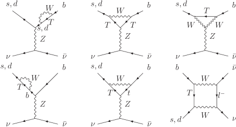
Figure 4: The Feynman diagrams of $T$-even heavy top quark $T$ contributing to the rare                 decay processes $b\rightarrow(s,d)\nu\bar{\nu}$ in the $LHT$ model.

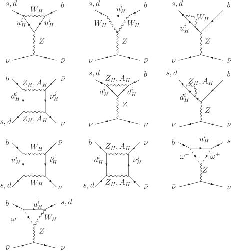
Figure 5: The Feynman diagrams of T-odd fermions contributing to the rare decay                  processes $b\rightarrow(s,d)\nu\bar{\nu}$ in the $LHT$ model.

The contributions of the $LHT$ model to the quark level transition processes $b\rightarrow d_{j}\nu\bar{\nu}(j=s,d)$ come from two new sources: $T$-even heavy top quark $T$ and the $T$-odd fermions, which can generate contributions to the coefficient $C^{\nu}_{L,SM}$. The relevant Feynman diagrams are shown in Fig.4 and Fig.5. From the discussions given in section 2, we can see that the $LHT$ model contributes to the rare decay processes $B\rightarrow M\nu\bar{\nu}$ ($M=\pi,K,\rho,K^{\ast}$) through the modification of the function $X_{SM}$ which is related to the coefficient $C^{\nu}_{L,SM}$.

It is obvious that the branching ratios $Br(B\rightarrow M\nu\bar{\nu})$ ($M=\pi,K,\rho,K^{\ast}$) contributed by the $LHT$ model are dependent on the free parameters $f$, $x_{L}$, the $T$-odd fermion masses $M_{Q^{i}_{H}}$, and the flavor mixing matrix elements $(V_{H_{d}})_{ij}$. The mixing matrix elements $(V_{H_{u}})_{ij}$ can be determined via $V_{H_{u}}=V_{H_{d}}V_{CKM}^{{\dagger}}$. The matrix $V_{H_{d}}$ can be parameterized in terms of three mixing angles and three phases, which can be probed by the $FCNC$ processes in $K$ and $B$ meson systems, as discussed in detail in Refs. [26, 10]. To avoid any additional parameters introduced and to simplify our calculations, we take $V_{H_{d}}=V_{CKM}$ and $V_{H_{u}}^{{\dagger}}=I$, and assume the $T$-odd fermion masses $M_{Q^{i}_{H}}$ in two scenarios:
Case I: $M_{Q^{1}_{H}}=M_{Q^{2}_{H}}=M_{Q^{3}_{H}}$.
Case II: The $T$-odd fermion masses $M_{Q^{i}_{H}}$ are not degenerate.

Case I is the $MFV$ limit of the $LHT$ model. In this case, the contributions of the $T$-odd fermions to the rare decay processes $B\rightarrow M\nu\bar{\nu}$ ($M=\pi,K,\rho,K^{\ast}$) equal to zero from the unitarity of the matrix $V_{H_{d}}$. The contributions of the $LHT$ model to these $FCNC$ processes are only coming from the $T$-even heavy top quark $T$, which are dependent on two parameters $x_{L}$ and $f$. The relative functions are given by[10, 11]

$$X_{SM}(x_{t}) = \frac{x_{t}}{8}\left[\frac{x_{t}+2}{x_{t}-1}+\frac{3x_{t}-6}{(x_{t}-1)^{2}}\log x_{t}\right],$$ (19)

$$\bar{X}_{even} = x^{2}_{L}\frac{\upsilon^{2}}{f^{2}}\left[U_{3}(x_{t},x_{T})+\frac{x_{L}}{1-x_{L}}\frac{x_{t}}{8}\right],$$ (20)

$$U_{3}(x_{t},x_{T}) = \frac{-3+2x_{t}-2x^{2}_{t}}{8(-1+x_{t})}-\frac{x_{t}(-4-x_{t}+2x^{2}_{t})\log x_{t}}{8(-1+x_{t})^{2}}+\frac{(3+2x_{t})\log x_{T}}{8},$$ (21)

where the parameters $x_{i}$ are defined as

$$x_{t} = \frac{m^{2}_{t}}{M^{2}_{W}},\quad\quad x_{T}=\frac{m^{2}_{T}}{M^{2}_{W}}.$$ (22)

For case II, the contributions of the $LHT$ model to the rare decay processes $B\rightarrow M\nu\bar{\nu}$ come from T-even and T-odd sectors. The expression forms of the functions $X_{i}$, which are related to our calculation, can be written as:

$$X_{s,d} = X_{SM}+\bar{X}_{even}+\frac{1}{\lambda_{t}^{s,d}}\bar{X}^{odd}_{s,d},$$ (23)

where the functions $X_{SM}$ and $\bar{X}_{even}$ have been given in Eq. (19) and Eq. (20), respectively, the function $\bar{X}^{odd}_{s,d}$ is [10, 11]

$$\bar{X}^{odd}_{s,d} = \left[\xi^{s,d}_{2}(J^{\nu\bar{\nu}}(z_{2},y)-J^{\nu\bar{\nu}}(z_{1},y))+\xi^{s,d}_{3}(J^{\nu\bar{\nu}}(z_{3},y)-J^{\nu\bar{\nu}}(z_{1},y))\right]$$ (24)

with

$$J^{\nu\bar{\nu}}(z_{i},y) = \frac{1}{64}\frac{\upsilon^{2}}{f^{2}}\left[z_{i}S_{odd}+F^{\nu\bar{\nu}}(z_{i},y;W_{H})\right.$$ (25)

$$+\left.4\left(G(z_{i},y;Z_{H})+G_{1}(z^{\prime}_{i},y^{\prime};A_{H})+G_{2}(z_{i},y;\eta)\right)\right],$$

$$S_{odd} = \frac{z_{i}^{2}-2z_{i}+4}{(1-z_{i})^{2}}\log z_{i}+\frac{7-z_{i}}{2(1-z_{i})},$$ (26)

$$\xi^{s,d}_{2} = \lambda_{c}^{s,d},\quad\quad\xi^{s,d}_{3}=\lambda_{t}^{s,d},$$ (27)

$$\lambda_{c}^{s} = V^{\ast}_{cb}V_{cs},\quad\lambda_{c}^{d}=V^{\ast}_{cb}V_{cd},\quad\lambda_{t}^{s}=V^{\ast}_{tb}V_{ts},\quad\lambda_{t}^{d}=V^{\ast}_{tb}V_{td}.$$ (28)

Here the functions $F^{\nu\bar{\nu}},G,G_{1}$ and $G_{2}$ given in Appendix and the various variables defined as follows

$$z_{i} = \frac{M^{2}_{Q^{i}_{H}}}{M_{W_{H}}^{2}}=\frac{M^{2}_{Q^{i}_{H}}}{M_{Z_{H}}^{2}},\quad\quad z^{\prime}_{i}=az_{i},\quad\quad a=\frac{5}{\tan^{2}\theta_{w}},$$ (29)

$$y = \frac{M^{2}_{L_{H}}}{M_{W_{H}}^{2}}=\frac{M^{2}_{L_{H}}}{M_{Z_{H}}^{2}},\quad\quad y^{\prime}=ay,\quad\quad\eta=\frac{1}{a}\quad.$$ (30)

The mass of the T-odd heavy gauge boson $W_{H}$ can be written as $M_{W_{H}}=fg(1-\frac{\upsilon^{2}}{8f^{2}})$ and there is $M_{W_{H}}\simeq M_{Z_{H}}$.

In the context of the $LHT$ model, the branching ratios of the rare decays $B\rightarrow X_{s,d}\nu\bar{\nu}$ can be written as:

$$\mathcal{B}(B\rightarrow X_{s}\nu\bar{\nu}) = \left|\frac{X_{s}}{X_{SM}}\right|^{2}\mathcal{B}(B\rightarrow X_{s}\nu\bar{\nu})_{SM},$$ (31)

$$\mathcal{B}(B\rightarrow X_{d}\nu\bar{\nu}) = \left|\frac{X_{d}}{X_{SM}}\right|^{2}\mathcal{B}(B\rightarrow X_{d}\nu\bar{\nu})_{SM}.$$ (32)

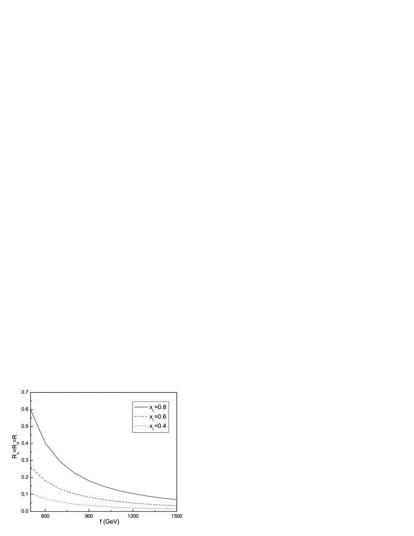
Figure 6: The relative correction parameter $R$ as a function of the scale parameter $f$ for                three value of the mixing parameter $x_{L}$ in case I.

(a)

(b)

(c) Same as Fig.6 but for case II.

To see the contributions of the $LHT$ model to the rare decays $B\rightarrow X_{s,d}\nu\bar{\nu}$, we define the relative correction parameters $R_{s}$ and $R_{d}$ as

$$R_{s} = \frac{\mathcal{B}(B\rightarrow X_{s}\nu\bar{\nu})-\mathcal{B}(B\rightarrow X_{s}\nu\bar{\nu})_{SM}}{\mathcal{B}(B\rightarrow X_{s}\nu\bar{\nu})_{SM}}=\frac{X_{s}^{2}-X_{SM}^{2}}{X_{SM}^{2}},$$ (33)

$$R_{d} = \frac{\mathcal{B}(B\rightarrow X_{d}\nu\bar{\nu})-\mathcal{B}(B\rightarrow X_{d}\nu\bar{\nu})_{SM}}{\mathcal{B}(B\rightarrow X_{d}\nu\bar{\nu})_{SM}}=\frac{X_{d}^{2}-X_{SM}^{2}}{X_{SM}^{2}}.$$ (34)

For case I, because the contributions of $T$-odd particles disappear and the contributions of the $LHT$ model to the rare decay processes $B\rightarrow M\nu\bar{\nu}$ only come from the $T$-even heavy top quark $T$ which are dependent on the free parameters $x_{L}$ and $f$. If we see these processes at the quark level, we can obtain $X_{s}=X_{d}$ and thus there is $R_{s}=R_{d}$. For case II, both $T$-even and $T$-odd particles can contribute to these $FCNC$ decay processes. From Eqs. (24)–(28), we can see that the functions $X_{s}$ and $X_{d}$ are different from each other due to $\frac{1}{\lambda_{t}^{s,d}}\bar{X}^{odd}_{s,d}$. Thus, in case II, the T-odd fermion masses not being degenerate, there is $R_{s}\neq R_{d}$.

Our numerical results are summarized in Fig.6 and Fig.7 for case I and case II, respectively. In Fig.6, we have assumed $R_{s}=R_{d}=R$, in Fig.7 we have taken $M_{Q^{1}_{H}}=700~{}\rm GeV$, $M_{Q^{2}_{H}}=1000~{}\rm GeV$, $M_{Q^{3}_{H}}=1500~{}\rm GeV$ and $M_{L_{H}}=500~{}\rm GeV$. One can see from Fig.6 and Fig.7 that the contributions of the $LHT$ model to the rare $B$ decays $B\rightarrow M\nu\bar{\nu}(M=\pi,K,\rho,K^{\ast})$ are smaller than those of the $TC2$ model. For the scale parameter $f\geq 1TeV$ and the mixing parameter $x_{L}\leq 0.8$, the value of the correction parameter $R_{s}=R_{d}=R$ contributed by the $T$-even heavy top quark $T$ is smaller than $14.7\%$, which is consistent with the numerical result given by Fig.5 of Ref. [10]. In case II, the $T$-odd particles have contributions to the rare decay processes $B\rightarrow M\nu\bar{\nu}$. However, their contributions are smaller than those of the $T$-even heavy top quark $T$. For example, for $M_{Q^{1}_{H}}=700~{}\rm GeV$, $M_{Q^{2}_{H}}=1000~{}\rm GeV$, $M_{Q^{3}_{H}}=1500~{}\rm GeV$, $M_{L_{H}}=500~{}\rm GeV$, $f\geq 500GeV$, and $x_{L}\leq 0.8$, the value of the relative correction parameter $R_{s}$ contributed by the $T$-odd particles is smaller than $5\%$. Certainly, in this paper, we have taken $V_{H_{d}}=V_{CKM}$, which is a very limited scenario. In more general scenarios, as discussed in Ref. [10], the contributions of the $T$-odd particles can be enhanced. However, in most of the parameter space of the $LHT$ model, the value of the relative correction parameter $R_{s}$ or $R_{d}$ contributed by the $T$-odd particles is smaller than $10\%$. It is well known that the $SM$ prediction values for the branching ratios of the rare $B$ decays $B\rightarrow M\nu\bar{\nu}$ have large uncertainties. Thus, we have to say that it is very difficult to detect correction effects of the $LHT$ model on the rare $B$ decays $B\rightarrow M\nu\bar{\nu}$ in near future high energy collider experiments.

4. Conclusions

The $TC2$ model and the $LHT$ model are two kinds of popular new physics models beyond the $SM$. The new particles predicted by these two new physics models can induce $FC$ couplings to ordinary particles and thus can produce contributions to some $FCNC$ processes. The rare $B$ semileptonic decays with neutrinos in the final state are significantly suppressed in the $SM$ and their long-distance contributions are generally subleading. So these $FCNC$ processes are considered as excellent probes of new physics beyond the $SM$. In this paper, we consider the contributions of the $TC2$ model and the $LHT$ model to the rare $B$ decay processes $B\rightarrow M\nu\bar{\nu}$ with $M=\pi,\rho,K,K^{\ast}$ and discuss the possibility of constraining the relevant free parameters using the corresponding experimental upper limits. The following conclusions are obtained.

$i)$ The contributions of the $TC2$ model to these rare decay processes are larger than those from the $LHT$ model. We might use these processes to distinguish different new physics models in future high energy collider experiments.

$ii)$ The contributions of the $TC2$ model to these rare decay processes mainly come from the nonuniversal gauge boson $Z^{\prime}$. The contributions of $Z^{\prime}$ to the quark level transition processes $b\to sl^{+}l^{-}$ are correlated with those for the quark level transition processes $b\to s\nu\bar{\nu}$. However, even if the experimental measurement value of the branching ratio $Br(B\to X_{s}l^{+}l^{-})$ gives severe constraints on the relevant free parameters, it is still possible to largely enhance the branching ratios of the rare $B$ decay processes $B\rightarrow M\nu\bar{\nu}$ in the $TC2$ model.

$iii)$ The contributions of the nonuniversal gauge boson $Z^{\prime}$ to the rare $B$ decays $B\rightarrow V\nu\bar{\nu}$ are larger than those for the rare $B$ decays $B\rightarrow P\nu\bar{\nu}$. The experimental upper limits of the branching ratios for some of these rare decay processes can give constraints on the free parameters of the $TC2$ model. The most severe constraints on the free parameters of the $TC2$ model come from the rare $B$ decay $B^{+}_{u}\rightarrow K^{\ast+}\nu_{\tau}\bar{\nu_{\tau}}$, which demands that if we desire $M_{Z^{\prime}}=2~{}\rm TeV$, there must be $K_{1}\leq 0.5$.

$iv)$ In general, the contributions of the $LHT$ model to the rare $B$ decays $B\rightarrow M\nu\bar{\nu}$ come from two sources: the $T$-even and $T$-odd sectors. However, for the case that the $T$-odd fermions are degenerated in mass, the contributions only come from the $T$-even heavy top quark $T$. For $f\geq 1TeV$ and $x_{L}\leq 0.8$, the value of the correction parameter $R$ contributed only by $T$ is smaller than $14.7\%$. In most of the parameter space of the $LHT$ model, the value of the relative correction parameter $R_{s}$ or $R_{d}$ contributed by the $T$-odd particles is smaller than $10\%$.

Acknowledgments

This work is supported in part by the National Natural Science Foundation of China under Grant No.10975067, the Specialized Research Fund for the Doctoral Program of Higher Education(SRFDP) (No.200801650002), the Natural Science Foundation of Liaoning Science Committee(No.20082148), and the Foundation of Liaoning Educational Committee(No.2007T086).

Appendix

In this appendix we list the functions which are related to our calculation in the context of the $TC2$ and $LHT$ models. In the framework of the $TC2$ model:

$$C_{a}(x_{t}) = \frac{8}{3}(\tan^{2}\theta^{\prime}-1)\frac{F_{1}(x_{t})}{\upsilon_{d}+a_{d}},$$ (35)

$$C_{b}(x_{t}) = \frac{16F_{2}(x_{t})}{3(\upsilon_{u}-a_{u})}-\frac{8F_{3}(x_{t})}{3(\upsilon_{u}+a_{u})},$$ (36)

$$C_{c}(x_{t}) = \frac{16F_{4}(x_{t})}{3(\upsilon_{u}-a_{u})}+\frac{8F_{5}(x_{t})}{3(\upsilon_{u}+a_{u})}$$ (37)

with

$$F_{1}(x_{t}) = -(0.5(Q-1)\sin^{2}\theta_{w}+0.25)(x_{t}^{2}\ln(x_{t})/(x_{t}-1)^{2}+x_{t}/(x_{t}-1)$$ (38)

$$- x_{t}(0.5(-0.5772+\ln(4\pi)-\ln(M^{2}_{W}))+0.75-0.5(x_{t}^{2}\ln(x_{t})/(x_{t}-1)^{2}$$

$$- 1/(x_{t}-1))))((1+x_{t})/(x_{t}-2)),$$

$$F_{2}(x_{t}) = (0.5Q\sin^{2}\theta_{w}-0.25)(x_{t}^{2}\ln(x_{t})/(x_{t}-1)^{2}-2x_{t}\ln(x_{t})/(x_{t}-1)^{2}$$ (39)

$$+ x_{t}/(x_{t}-1)),$$

$$F_{3}(x_{t}) = -Q\sin^{2}\theta_{w}(x_{t}/(x_{t}-1)-x_{t}\ln(x_{t})/(x_{t}-1)^{2}),$$ (40)

$$F_{4}(x_{t}) = 0.25(4\sin^{2}\theta_{w}/3-1)(x^{2}_{t}\ln(x_{t})/(x_{t}-1)^{2}-x_{t}-x_{t}/(x_{t}-1)),$$ (41)

$$F_{5}(x_{t}) = -0.25Q\sin^{2}\theta_{w}x_{t}(-0.5772+\ln(4\pi)-\ln(M^{2}_{W})+1-x_{t}\ln(x_{t})/(x_{t}-1))$$ (42)

$$- \sin^{2}\theta_{w}/6(x^{2}_{t}\ln(x_{t})/(x_{t}-1)^{2}-x_{t}-x_{t}/(x_{t}-1)).$$

Here the variables are defined as: $\upsilon_{u,d}=I_{3}-2Q_{u,d}\sin^{2}\theta_{w},a_{u,d}=I_{3}$, where $u$ and $d$ represent the up- and down-type quarks, respectively. $I_{3}$ is the third component of isospin and $Q_{i}$ is the charge of the corresponding quark.

The form factors $f^{i}$ for the decay processes $B\rightarrow(K,\pi)\nu\bar{\nu}$ can be written as [17]:

$$f^{P}_{+}(s_{B}) = \frac{f(0)}{1-a_{f}(s_{B}/m^{2}_{B})+b_{f}(s_{B}/m^{2}_{B})^{2}},$$ (43)

$$f^{\pi}(0) = 0.258\pm 0.031,\quad\quad a^{\pi}_{f}=1.29,\quad\quad b^{\pi}_{f}=0.206,$$

$$f^{K}(0) = 0.331\pm 0.041,\quad\quad a^{K}_{f}=1.41,\quad\quad b^{K}_{f}=0.406.$$

The form factors for the decay processes $B\rightarrow(K^{\ast},\rho)\nu\bar{\nu}$ can be written as [18]:

$$A_{i}(s_{B}) = A_{i}(0)(1+\beta_{i}s_{B}),\quad\quad\beta_{1}=-0.023GeV^{-2},\quad\quad\beta_{2}=0.034GeV^{-2}.$$

$$V^{B\rightarrow K^{\ast}}(0) = 0.411\pm 0.033,\quad\quad A^{B\rightarrow K^{\ast}}_{1}(0)=0.292\pm 0.028,\quad\quad A^{B\rightarrow K^{\ast}}_{2}(0)=0.259\pm 0.025,$$

$$V^{B\rightarrow\rho}(0) = 0.323\pm 0.030,\quad\quad A^{B\rightarrow\rho}_{1}(0)=0.242\pm 0.023,\quad\quad A^{B\rightarrow\rho}_{2}(0)=0.221\pm 0.025.$$

In the $LHT$ model, the relevant functions can be written as [10, 11]:

$$F^{\nu\bar{\nu}}(z_{i},y;W_{H}) = \frac{3}{2}z_{i}-F_{5}(z_{i},y)-7F_{6}(z_{i},y)-9U(z_{i},y),$$ (44)

$$F_{5}(z_{i},y) = \frac{z_{i}^{3}\log z_{i}}{(1-z_{i})(y-z_{i})}+\frac{y^{3}\log y}{(1-y)(z_{i}-y)},$$ (45)

$$F_{6}(z_{i},y) = -\left[\frac{z_{i}^{2}\log z_{i}}{(1-z_{i})(y-z_{i})}+\frac{y^{2}\log y}{(1-y)(z_{i}-y)}\right],$$ (46)

$$U(z_{i},y) = \frac{z_{i}^{2}\log z_{i}}{(1-z_{i})^{2}(z_{i}-y)}+\frac{y^{2}\log y}{(1-y)^{2}(y-z_{i})}+\frac{1}{(1-z_{i})(1-y)},$$ (47)

$$G(z_{i},y;Z_{H}) = -\frac{3}{4}U(z_{i},y),$$ (48)

$$G_{1}(z^{\prime}_{i},y^{\prime};A_{H}) = \frac{1}{25a}G(z^{\prime}_{i},y^{\prime};A_{H}),$$ (49)

$$G_{2}(z_{i},y;\eta) = -\frac{3}{10a}\left[\frac{z_{i}^{2}\log z_{i}}{(1-z_{i})(\eta-z_{i})(z_{i}-y)}\right.$$ (50)

$$+\left.\frac{y^{2}\log y}{(1-y)(\eta-y)(y-z_{i})}+\frac{\eta^{2}\log\eta}{(1-\eta)(z_{i}-\eta)(\eta-y)}\right].$$

References

- [1] H. Tajima et al., Int. J. Mod. Phys. A17(2002)2967 ; R. Mizuk, R. Chistov et al., Phys. Rev. D78(2008)072004 ; B. Aubert et al., Phys. Rev. Lett. 100(2008)021801.
- [2] Y. Grossman, Z. Ligeti and E. Nardi, Nucl. Phys. B465(1996)369; Erratum-ibid, B480(1996)753; D. Melikhov, N. Nikitin and S. Simula, Phys. Lett. B428(1998)171; C. S. Kim, Y. G. Kim and T. Morozumi, Phys. Rev. D60(1999)094007; G. Buchalla, G. Hiller and G. Isidori, Phys. Rev. D63(2000)014015.
- [3] T. M. Aliev, A. Ozpineci and M. Savci, Phys. Lett. B506(2001)77; J. H. Jeon, C. S. Kim, J. Lee and C. Yu, Phys. Lett. B636(2006)270; T. M. Aliev, A. S. Cornell and N. Gaur, JHEP 0707(2007)072; Y. Yamada, Phys. Rev. D77(2008)014025; C. S. Kim, S. C. Park, K. Wang, G. Zhu, arXiv:0910.4291 [hep-ph]; M. Blanke, A. J. Buras, B. Duling, K. Gemmler and S. Gori, JHEP 0903(2009)108; J. F. Kamenik and C. Smith, Phys. Lett. B680(2009)471.
- [4] W. Altmannshofer, A. J. Buras, D. M. Straub and M. Wick, JHEP 0904(2009)022.
- [5] M. Bona et al., arXiv:0709.0451[hep-ex].
- [6] C. T. Hill, Phys. Lett. B345(1995)483; K. D. Lane and E. Eichten, Phys. Lett. B352(1995)382; K. D. Lane, Phys. Lett. B433(1998)96; G. Cvetic, Rev. Mod. Phys. 71(1999)513.
- [7] N. Arkani-Hamed, A. G. Cohen and H. Georgi, Phys. Rev. Lett 86(2001)4757; N. Arkani-Hamed, A. G. Cohen and H. Georgi, Phys. Lett. B513(2001)232; N. Arkani-Hamed, A. G. Cohen, E. Katz and A. E. Nelson, JHEP 0207(2002)034.
- [8] M. Schmaltz and D. Tucker-Smith, Ann. Rev. Nucl. Part. Sci. 55(2005)229; M. Perelstein, Prog. Part. Nucl. Phys. 58(2007)247.
- [9] H. C. Cheng, I. Low, JHEP 0309(2003)051; JHEP 0408(2004)061; I. Low, JHEP 0410(2004)067.
- [10] M. Blanke et al., JHEP 0701(2007)066.
- [11] T. Goto, Y. Okada and Y. Yamamoto, Phys. Lett. B670(2009)378; F. del Aguila, J. I. Illana and M. D. Jenkins, JHEP 0901(2009)080; M. Blanke et al., arXiv:0906.5454[hep-ph].
- [12] C. T. Hill and E. H. Simmons, Phys. Rept. 381(2003)235; Erratum -ibid, 390(2004)553.
- [13] G. Buchalla, G. Burdman, C. T. Hill and D. Kominis, Phys. Rev. D53(1996)5185.
- [14] P. Colangelo, F. De Fazio, P. Santorelli, E. Scrimieri, Phys. Lett. B395(1997)339.
- [15] T. Inami, C. S. Lim, Prog. Theor. Phys. 65(1981)297; A. J. Buras, arXiv:9806471[hep-ph].
- [16] C. S. Kim and R. M. Wang, Phys. Lett. B681(2009)44.
- [17] P. Ball, R. Zwicky, Phys. Rev. D71(2005)014015.
- [18] P. Ball, R. Zwicky, Phys. Rev. D71(2005)014029.
- [19] W. M. Yao et al.[Particle Date Group], J. Phy. G33(2006)1 and 2007 partial update for 2008 edition.
- [20] R. S. Chivukula and E. H. Simmons, Phys. Rev. D66(2002)015006.
- [21] M. B. Popovic and E. H. Simmons, Phys. Rev. D58(1998)095007; G. Burdman and N. J. Evens, Phys. Rev. D59(1999)115005.
- [22] H. J. He, C. P. Yuan, Phys. Rev. Lett. 83(1999)28; G. Burdman, Phys. Rev. Lett. 83(1999)2888.
- [23] Wei Liu, Chong-Xing Yue, Hui-Di Yang, Phys. Rev. D79(2009)034008.
- [24] B. Aubert et. al.[BaBar Collaboration] , Phys. Rev. Lett. 93(2004)081802; M. Iwasaki et. al.[Belle Collaboration], Phys. Rev. D72(2005)092005.
- [25] J. Hubisz, P. Meade, Phys. Rev. D71(2005)035016; J. Hubisz, P. Meade, A. Noble and M. Perelstein, JHEP 0601(2006)135.
- [26] J. Hubisz, S. J. Lee and G. Paz, JHEP 0606(2006)041; M. Blanke et al., Phys. Lett. B646(2007)253.