A Gravitational Redshift Determination of the Mean Mass of White Dwarfs. DA Stars

Abstract

We measure apparent velocities ($v_{\rm app}$) of the H$\alpha$ and H$\beta$ Balmer line cores for 449 non-binary thin disk normal DA white dwarfs (WDs) using optical spectra taken for the ESO SN Ia Progenitor surveY (SPY; Napiwotzki et al., 2001). Assuming these WDs are nearby and co-moving, we correct our velocities to the Local Standard of Rest so that the remaining stellar motions are random. By averaging over the sample, we are left with the mean gravitational redshift, $\langle v_{\rm g}\rangle$: we find $\langle v_{\rm g}\rangle=\langle v_{\rm app}\rangle=32.57\pm 1.17$ km s^-1. Using the mass-radius relation from evolutionary models, this translates to a mean mass of $0.647^{+0.013}_{-0.014}$ M_⊙. We interpret this as the mean mass for all DAs. Our results are in agreement with previous gravitational redshift studies but are significantly higher than all previous spectroscopic determinations except the recent findings of Tremblay & Bergeron (2009). Since the gravitational redshift method is independent of surface gravity from atmosphere models, we investigate the mean mass of DAs with spectroscopic $T_{\rm eff}$ both above and below 12000 K; fits to line profiles give a rapid increase in the mean mass with decreasing $T_{\rm eff}$. Our results are consistent with no significant change in mean mass: $\langle M\rangle$ ${}^{\rm hot}=0.640\pm 0.014$ M_⊙ and $\langle M\rangle$ ${}^{\rm cool}=0.686^{+0.035}_{-0.039}$ M_⊙.

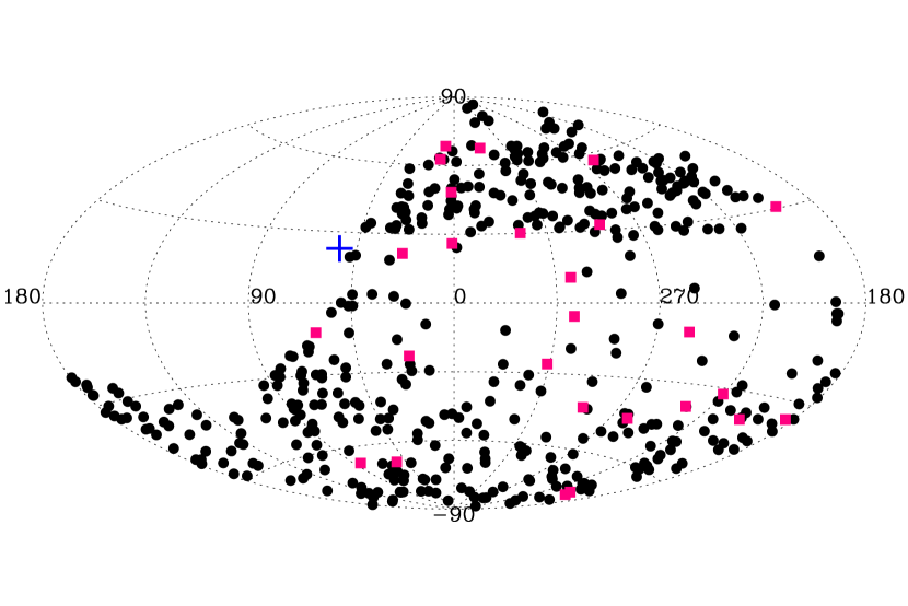
Figure 1.— Distribution of targets in Galactic longitude $l$ and latitude $b$. We mark the targets in our main sample as black points and the thick disk WDs as pink squares. We indicate the direction of the movement of the Sun with respect to the LSR (blue cross ; Kerr & Lynden-Bell, 1986). Since the observations are from the ESO VLT in the Southern Hemisphere, no targets with a declination above $+30^{\circ}$ are in our sample, hence the gap in the left side of the plot.

1. Introduction

Nearly all stars end their trek through stellar evolution by becoming white dwarfs (WDs). Hence, properties of WDs can provide important information on the chemical and formation history of stars in our Galaxy, as well as on the late stages of stellar evolution. Of these stellar properties mass is one of the most fundamental, and though there are several methods for mass determination of WDs, each has its limitations.

The most-widely used WD mass determination method involves comparing predictions from atmosphere models with observations to obtain effective temperatures ($T_{\rm eff}$) and/or surface gravities (log $g$). One can then compare these quantities with predictions from evolutionary models (e.g., Althaus & Benvenuto, 1998; Montgomery et al., 1999). Shipman (1979), Koester et al. (1979), and McMahan (1989) use radii determined from trigonometric parallax measurements along with $T_{\rm eff}$ from photometry to determine masses. Of course this technique is limited to target stars with measured parallaxes, so users of photometry have more often used observed color indices to determine both $T_{\rm eff}$ and log $g$ (e.g., Koester et al., 1979; Wegner, 1979; Shipman & Sass, 1980; Weidemann & Koester, 1984; Fontaine et al., 1985). With the exception of the parallax variant (Kilic et al., 2008), the photometric method is seldom used in recent WD research.

Another variant of this method uses mainly spectroscopic rather than photometric observations (e.g., Bergeron et al., 1992; Finley et al., 1997; Liebert et al., 2005). With more recent large-scale surveys, such as SPY (see Section 3) and the Sloan Digital Sky Survey (SDSS; York et al., 2000), the comparison of observed WD spectra with spectral energy distributions of theoretical atmosphere models has become the primary WD mass determination method, yielding masses for a large number of WDs (e.g., Koester et al., 2001; Madej et al., 2004; Kepler et al., 2007).

When applied to cool WDs ($T_{\rm eff}\lesssim 12000$ K), however, the reliability of this primary method breaks down: a systematic increase in the mean log $g$ for DAs with lower $T_{\rm eff}$ has repeatedly shown up in analyses (e.g., Liebert et al., 2005; Kepler et al., 2007; DeGennaro et al., 2008). This “log $g$ upturn”, discussed thoroughly by Bergeron et al. (2007) and by Koester et al. (2009a), is generally believed to reflect shortcomings of the atmosphere models $-$ specifically our understanding of the line profiles $-$ rather than a real increase in mean mass with decreasing $T_{\rm eff}$ as an increasing mean log $g$ would imply.

Other mass determination methods that are independent of atmosphere models include the astrometric technique (e.g., Gatewood & Gatewood, 1978) and pulsational mode analysis (e.g., Winget et al., 1991). Unfortunately, neither of these methods are widely applicable to WDs. The former requires stellar systems with multiple stars, and the latter is limited to WDs and pre-white dwarfs which lie in narrow $T_{\rm eff}$ ranges of pulsational instability.

Another method that is mostly atmosphere model-independent uses the gravitational redshift of absorption lines; this is the one that will be the focus of this paper. The difficulty in disentangling the stellar radial velocity shift from the gravitational redshift has caused this method to only be used for WDs in common proper motion binaries or open clusters (Greenstein & Trimble, 1967; Koester, 1987; Wegner & Reid, 1991; Reid, 1996; Silvestri et al., 2001). The simplicity of this method, however, prompts us to extend the investigation beyond those cases.

In this paper, we will make two main points: (1) by using a large, high-resolution spectroscopic dataset, we can circumvent the radial velocity-gravitational redshift degeneracy to measure a mean gravitational redshift of WDs in our sample and use that to arrive at a mean mass; and (2) since the gravitational redshift method has the advantage of being independent of surface gravity from atmosphere models, we can use it to reliably probe cool DAs ($T_{\rm eff}\lesssim 12000$ K), thus providing important insight into the “log $g$ upturn problem” as groups continue to improve upon those models (e.g., Tremblay & Bergeron, 2009).

2. Gravitational Redshift

In the weak-field limit, the general relativistic effect of gravitational redshift ($z$) can be understood, classically, as the energy ($E$) lost by a photon as it escapes a gravitational potential ($\Phi$) well:

$$z=\frac{-\Delta E}{E}=\frac{-\Phi}{c^{2}}.$$ (1)

The fractional change in energy can be rewritten as a fractional change in observed wavelength ($-\Delta E/E=\Delta\lambda/\lambda$). In our case, the gravitational potential is at the surface of a WD of mass $M$ and radius $R$. In terms of a velocity, the gravitational redshift is

$$v_{g}=\frac{c\Delta\lambda}{\lambda}=\frac{GM}{Rc}$$ (2)

where $G$ is the gravitational constant, and $c$ is the speed of light.

For WDs, $v_{\rm g}$ is comparable in magnitude to the stellar radial velocity $v_{\rm r}$, both of which sum to give the apparent velocity we measure from absorption lines: $v_{\rm app}=v_{\rm g}+v_{\rm r}$. These two components cannot be explicitly separated for individual WDs without an independent $v_{\rm r}$ measurement or mass determination.

The method of this paper is to break this degeneracy not for individual targets but for the sample as a whole. We make the assumption that our WDs are a co-moving, local sample. After we correct each $v_{\rm app}$ to the Local Standard of Rest (LSR), only random stellar motions dominate the dynamics of our sample. We assume, for the purposes of this investigation, that these average out. Thus the mean apparent velocity equals the mean gravitational redshift: $\langle v_{\rm app}\rangle=\langle v_{\rm g}\rangle$. The idea of averaging over a group of WDs to extract a mean gravitational redshift is not new (Greenstein & Trimble, 1967), but the availability of an excellent dataset prompted its exploitation. We address the validity of the co-moving approximation in Section 4.1.

3. Observations

We use spectroscopic data from the European Southern Observatory (ESO) SN Ia Progenitor surveY (SPY; Napiwotzki et al., 2001). These observations, taken using the UV-Visual Echelle Spectrograph (UVES; Dekker et al., 2000) at Kueyen, Unit Telescope 2 of the ESO VLT array, constitute the largest, homogeneous, high-resolution (0.36 Å or $\sim 16$ km s^-1 at H$\alpha$) spectroscopic dataset for WDs. We obtain the pipeline-reduced data online through the publicly available ESO Science Archive Facility.

3.1. Sample

As explained in Napiwotzki et al. (2001), targets for the SPY sample come from: the white dwarf catalog of McCook & Sion (1999), the Hamburg ESO Survey (HES; Wisotzki et al., 2000; Christlieb et al., 2001), the Hamburg Quasar Survey (Hagen et al., 1995; Homeier et al., 1998), the Montreal-Cambridge-Tololo survey (MCT; Lamontagne et al., 2000), and the Edinburgh-Cape survey (EC; Kilkenny et al., 1997). The magnitude of the targets is limited to $B<16.5$.

Our main sample consists of 449 analyzed hydrogen-dominated WDs (see Figure 1 for the distribution of targets in Galactic coordinates). This is the subset of the SPY sample that meets our sample criteria (explained below) and that shows measurable $v_{\rm app}$ in the H$\alpha$ (and H$\beta$) line cores while not showing measurable $v_{\rm app}$ variations. A variable velocity across multiple epochs of observation suggests binarity. The method of SPY to search for double degenerate systems is to detect variable radial velocity. For our study, however, we are interested only in non-binary WDs since these presumably have no radial velocity component in addition to random stellar motion after being corrected to the LSR. We exclude known double degenerates and common proper motion binary systems (Finley & Koester, 1997; Jordan et al., 1998; Maxted & Marsh, 1999; Maxted et al., 2000; Silvestri et al., 2001; Koester et al., 2009b) even if we do not find them to show variable $v_{\rm app}$.

We choose “normal” DAs (criterion 1) from Koester et al. (2009b). Classification as a normal DA does not include WDs that exhibit He absorption in their spectra in addition to H absorption, and it does not include magnetic WDs. In a subsequent paper we will investigate the sample of 20 helium-dominated WDs for which we observe H absorption.

For our main sample, we are also only interested in thin disk WDs (criterion 2), so we exclude halo and thick disk candidates as kinematically classified by Pauli et al. (2006) and Richter et al. (2007). We assume the rest are thin disk objects, the most numerous Galactic component. Our sample selection is also consistent with the results for the targets in common with Sion et al. (2009). Richter et al. (2007) find only 2% and 6% of their 632 DA WDs from SPY to be from the halo and thick disk, respectively. For WDs within 20 pc, Sion et al. (2009) find no evidence for halo objects and virtually no thick disk objects. We note that unique identification of population membership for WDs is difficult and often not possible because of ambiguous kinematical properties. Based on corrections for these intrinsic contaminations by Napiwotzki (2009), we expect any residual contamination in our sample to be at most $\sim 6$%. A contamination this size will have a negligible impact on our conclusions. We explain the significance of requiring thin disk WDs in Section 4.1, and we explore a mini-sample of thick disk WDs in Section 5.4.

The gravitational redshift method becomes very difficult for hot DAs with $50000$ K $\gtrsim T_{\rm eff}\gtrsim 40000$ K (see the $T_{\rm eff}$ gap in Figure 6). As the WD cools through this $T_{\rm eff}$ range, the Balmer line core, which we use to measure $v_{\rm app}$ (Section 4), disappears as it transitions from emission to absorption; fortunately only $\sim 5\%$ of the DAs from SPY lie in this range.

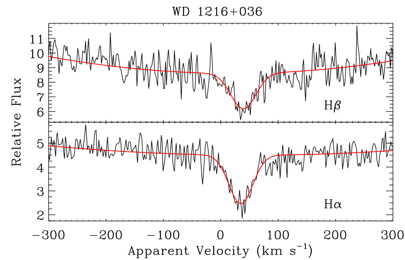
Figure 2.— Example UVES spectrum for a target in our sample. We measure $v_{\rm app}$ by fitting Gaussian profiles (solid, red lines) to the non-LTE Balmer line cores using a non-linear least-squares fitting routine. The line cores are well-resolved, allowing for precise centroid determinations.

4. Velocity Measurements

In the wings of absorption lines, and in particular, for the hydrogen Balmer series, the effects of collisional broadening cause asymmetry, making it difficult to measure a velocity centroid (Shipman & Mehan, 1976; Grabowski et al., 1987). These effects are much less significant, however, in the sharp, non-LTE line cores, and furthermore with decreasing principal quantum number, making both the H$\alpha$ and H$\beta$ line cores suitable options for measuring an apparent velocity $v_{\rm app}$. Higher order Balmer lines are intrinsically weaker (the H$\gamma$ line core, for example, is seldom observable in our data), so finite S/N prevents the number of observable H$\beta$ line cores from matching the number of observable H$\alpha$ line cores.

We measure $v_{\rm app}$ for each target in our sample by fitting a Gaussian profile to the H$\alpha$ line core using GAUSSFIT, a non-linear least-squares fitting routine in IDL (see Figure 2 for an example). When available, we combine this measurement with that of the H$\beta$ line core centroid as a mean weighted according to the uncertainties returned by the fitting routine. We include H$\beta$ line core centroid information in 372 of our 449 $v_{\rm app}$ measurements. If multiple epochs of observations exist, we combine these measurements as a weighted mean as well. Apparent velocity measurements of a given observation (i.e., H$\alpha$ and H$\beta$ line core centroids) are combined before multiple epochs.

Table 1 (full version available on-line) shows our measured $v_{\rm app}$ for H$\alpha$ and H$\beta$ (when observed) for each observation.

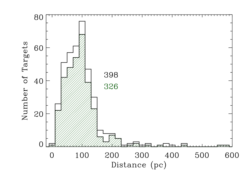
Figure 3.— Distribution of distances (from spectroscopic parallax) of SPY WDs from Pauli et al. (2006). The shaded, green histogram shows the targets in our sample. The mean is 94.5 pc; the median is 89.2 pc. These distances are short enough to support our co-moving approximation. We list the number of targets in each distribution.

4.1. Co-Moving Approximation

We measure a mean gravitational redshift by assuming that our WDs are a co-moving, local sample. With this assumption, only random stellar motions dominate the dynamics of our targets; this falls out when we average over the sample.

For this assumption to be valid, at least as an approximation, our WDs must belong to the same kinematic population; in the case of this work, this is the thin disk. We achieve a co-moving group by correcting each measured $v_{\rm app}$ to the kinematical LSR described by Standard Solar Motion (Kerr & Lynden-Bell, 1986).

There are reasons to believe that the targets in our sample will not significantly lag behind our choice of LSR due to asymmetric drift. Although WDs are considered “old” since they are evolved stars, it is the total age of the star (main sequence lifetime $\tau_{\rm nuc}$ and cooling time $\tau_{\rm cool}$) that is of consequence. WDs with $M\sim 0.6$ M_⊙ have main sequence progenitors with $M\sim 2$ M_⊙ (e.g., Williams et al., 2009). This corresponds to $\tau_{\rm nuc}\sim 1.4$ Gyr (Girardi et al., 2000). $\tau_{\rm cool}$ is on the order of a few hundred million years for most of the WDs in our sample ($T_{\rm eff}$ of a few times $10^{4}$ K) and $\sim 2.5\times 10^{9}$ yr for our coolest WDs ($T_{\rm eff}\sim 7000$ K); the total age spans a range of roughly 1.5 to 4 Gyr (F/G type stars).

We also make certain that our WDs reside at distances that are small when compared to the size of the Galaxy, thereby making systematics introduced by the Galactic kinematic structure negligible. Figure 3 shows the distances (from spectroscopic parallax; Pauli et al., 2006) to the targets in our sample. The mean distance of the targets in the histogram is less than 100 pc, and all are within 600 pc. Over these distances, the velocity dispersion with varying height above the disk remains modest (Kuijken & Gilmore, 1989), and differential Galactic rotation changes very little as well ($\sim 3$ km s^-1; Fich et al., 1989). In Section 5.3.2, we perform an empirical check to the assumptions made in this section.

5. Results

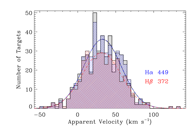
Figure 4.— Histograms of measured apparent velocities $v_{\rm app}$ with a bin size of 5 km s^-1. The mean $v_{\rm app}$ for all targets in our sample (shaded) is $32.57\pm 1.17$ km s^-1; the median is $31.94$ km s^-1; the standard deviation is $24.84$ km s^-1. Using $v_{\rm app}$ measured from H$\alpha$ only (red, descending lines): the mean $v_{\rm app}$ is $32.69\pm 1.18$ km s^-1; the median is $32.05$ km s^-1; the standard deviation is $24.87$ km s^-1. Using $v_{\rm app}$ measured from H$\beta$ only (blue, ascending lines): the mean $v_{\rm app}$ is $31.47\pm 1.32$ km s^-1; the median is $31.55$ km s^-1; the standard deviation is $25.52$ km s^-1. The overplotted curves are the Gaussian distribution functions used to determine Monte Carlo uncertainties. We list the number of targets in each distribution.

5.1. Mean Apparent Velocities

We present the distribution of our measured apparent velocities in Figure 4. Table 1 lists individual apparent velocity measurements, and mean apparent velocities are in Table 3.

Though our main method uses information from both the H$\alpha$ (Column 7 of Table 1) and H$\beta$ (Column 9) line cores to determine $v_{\rm app}$ for a given observation (Column 11), we also perform our analysis using H$\alpha$ only and H$\beta$ only. We measure H$\beta$ line core centroids for 382 of our 449 targets.

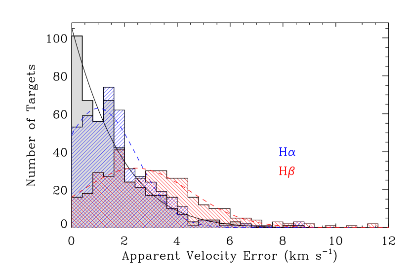
Figure 5.— Histograms of apparent velocity measurement uncertainties $\delta v_{\rm app}$ corresponding to the samples in Figure 4. The bin size is 0.4 km s^-1. The overplotted curves are the empirical distribution functions used to determine Monte Carlo uncertainties. Notice that measurements of the H$\alpha$ line core are more precise than for H$\beta$. For aesthetics, we leave off two H$\beta$ $\delta v_{\rm app}$ of 13.06 and 17.57 km s^-1.

Figure 5 shows the distribution of measurement uncertainties associated with each target. H$\beta$ centroid determinations are typically less precise than those for H$\alpha$ (see Column 6 of Table 3), which is expected since the H$\alpha$ line core is nearly always better-defined. We find that the improved precision achieved by combining H$\alpha$ and H$\beta$ information is not significant when determining the uncertainties to our mean apparent velocities. These uncertainties are dominated by sample size. In fact, we must increase (worsen) our typical measurement error of $\sim 2$ km s^-1 to $\sim 10$ km s^-1 to notice a $\sim 7\%$ increase in the error of the mean; a monstrous leap to measurement uncertainties of $\sim 50$ km s^-1 enlarges the error of the mean by a little more than a factor of 2. Thus, using H$\alpha$ (or H$\beta$) centroids only is sufficient for the kind of investigation employed in this paper, and lower resolution observations are also suitable as long as the Balmer line core is resolved.

The quoted uncertainties of the mean apparent velocities (Column 4 of Table 3) come from Monte Carlo simulations. For each sample, we recreate a large number of instances (10000) of the $v_{\rm app}$ distribution by randomly sampling from a convolution of the empirical $v_{\rm app}$ distribution (Gaussian characterized by the parameters in Columns 3 and 5 of Table 3) and the empirical measurement error distribution. We adopt the standard deviation of the resulting simulated mean values as our formal uncertainties. Since the input distributions for our simulations are empirical, our uncertainties are subject to the normal limitations of Frequentist statistics. We plot the empirical distribution of our main sample in Figure 4 (black curve) along with the distributions for the H$\alpha$ (dashed, blue curve) and H$\beta$ (dashed, red curve) samples. The corresponding empirical distributions of our measurement uncertainties are in Figure 5.

For convenience, Table 3 also lists the quantity $\langle M/R\rangle$, which is proportional to $\langle v_{\rm g}\rangle$ (equation 2) and, as we argue in Section 4.1, $\langle v_{\rm app}\rangle$.

5.2. Mean Masses

The mean apparent velocity $\langle v_{\rm app}\rangle$ (or $\langle M/R\rangle$) is our fundamental result since it is this quantity that is model-independent. To translate this to a mean mass (Table 4), we must invoke two dependencies: (1) we need an evolutionary model to give us a mass-radius relation, and (2) since the WD radius does slightly contract during its cooling sequence, we need an estimate of the position along this track for the average WD in our sample (i.e., a mean $T_{\rm eff}$).

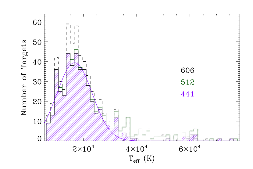
Figure 6.— Distribution of spectroscopically determined $T_{\rm eff}$ of normal DAs from Koester et al. (2009b) (dashed, black histogram). The bin size is 1500 K. The solid, green histogram shows the non-binary thin disk SPY targets, and the shaded, purple histogram shows the targets in our sample. The mean is $19400\pm 300$ K; the median is 17611 K.; the standard deviation is 9950 K. The overplotted curve is the empirical distribution function used to determine Monte Carlo uncertainties. We list the number of targets in each distribution.

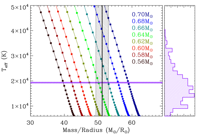
Figure 7.— (left) Plot of $M/R$ versus $T_{\rm eff}$ with cooling tracks from evolutionary models for a range of WD masses. The intersection of the mean measured apparent velocity $v_{\rm app}$ (vertical, black line) and mean $T_{\rm eff}$ from Figure 6 (horizontal, purple line) indicates a mean mass of $0.647^{+0.013}_{+0.014}$ M_⊙. (right) A version of Figure 6 with an abbreviated temperature range. We leave off 13 WDs with $T_{\rm eff}>50000$ K from the plot.

Our evolutionary models use $M_{\rm He}/M_{\star}=10^{-2}$ and $M_{\rm H}/M_{\star}=10^{-4}$ for the surface-layer masses; these are canonical values derived from evolutionary studies (e.g., Lawlor & MacDonald, 2006). See Montgomery et al. (1999) for a more complete description of our models. Our dependency on evolutionary models is small. We are interested in the mass-radius relation from these models, and this is relatively straight-forward since WDs are mainly supported by electron degeneracy pressure, making the WD radius a weak function of temperature. We estimate that varying the C/O ratio in the core affects the radius by less than 0.5%, whereas changing $M_{\rm H}/M_{\star}$ from $10^{-4}$ to $10^{-8}$ results in about a 4% decrease in radius. See Section 5.3.1 for more discussion on the dependency of the hydrogen layer mass.

Figure 7 plots $M/R$ versus $T_{\rm eff}$ with cooling tracks from evolutionary models for a range of WD masses. We use $\langle T_{\rm eff}\rangle=19400\pm 300$ K from the spectroscopically determined values of Koester et al. (2009b) (see Figure 6), and, after plotting $\langle M/R\rangle$ from Table 3, we interpolate to arrive at a mean mass of $0.647^{+0.013}_{-0.014}$ M_⊙ for 449 non-binary thin disk normal DA WDs from the SPY sample.

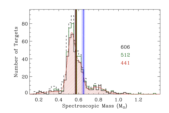
Figure 8.— Distribution of spectroscopic masses of normal DAs from Koester et al. (2009b) we derive using the published atmospheric parameters log $g$ and $T_{\rm eff}$ (dashed, black histogram). The bin size is 0.025 M_⊙. The solid, green histogram shows the non-binary thin disk SPY targets, and the shaded, orange histogram shows the targets in our sample. The means are $0.567\pm 0.002$ M_⊙ (vertical, black line), $0.580\pm 0.002$ M_⊙ (vertical, green line), and $0.575\pm 0.002$ M_⊙ (vertical, orange line), respectively. Notice that the mean spectroscopic masses are similar, indicating that the application of our sample criteria to SPY is not introducing additional systematic effects. All the means are also significantly less than the mean mass derived from the gravitational redshift method (vertical, blue line). The overplotted curve is the empirical distribution function used to determine Monte Carlo uncertainties. We list the number of targets in each distribution.

To compare this result with that of the spectroscopic method, we use atmospheric parameters log $g$ and $T_{\rm eff}$ from Koester et al. (2009b) along with the mass-radius relation from evolutionary models to derive individual masses for 441 of the targets in our sample (Koester et al. (2009b) do not publish individual WD masses). We derive a sharply peaked mass distribution (Figure 8) with width (not uncertainty) $\sigma=0.13$ M_⊙ and a mean mass of $0.575\pm 0.002$ M_⊙ $-$ significantly lower than the value we obtain from the gravitational redshift method. We compute the error of the mean using Monte Carlo simulations following the same method described in Section 5.1 except instead of using a single Gaussian to represent the mass distribution, we use multiple Gaussians (curve in Figure 8).

5.3. Systematic Effects

5.3.1 From Evolutionary Models

The hydrogen layer mass in DAs is believed to be in the range of $10^{-4}\gtrsim M_{\rm H}/M_{\star}\gtrsim 10^{-8}$, constrained by hydrogen shell burning in the late stages of stellar evolution (Althaus et al., 2002; Lawlor & MacDonald, 2006) and convective mixing (Fontaine & Wesemael, 1997). In their asteroseismological studies, Bischoff-Kim et al. (2008) also find evidence to support this range of hydrogen layer masses, and this is consistent with the results of Castanheira & Kepler (2009).

Our evolutionary models use the fiducial value of $M_{\rm H}/M_{\star}=10^{-4}$ for “thick” hydrogen layers. First, this is suggested by the pre-white dwarf evolutionary models of, e.g., Lawlor & MacDonald (2006), who find that the overwhelming majority of their DA models have thick hydrogen layers. Second, if thin layers were the norm, then convective mixing below 10000 K would lead to a disappearance of DAs at these temperatures (Fontaine & Wesemael, 1997). Both of these reasons lead us to choose thick hydrogen layers for our models.

We find that using a midrange hydrogen layer mass of $M_{\rm H}/M_{\star}=10^{-6}$ decreases the mean mass we derive for our main sample by $0.012$ M_⊙, while using a thin layer mass of $M_{\rm H}/M_{\star}=10^{-8}$ decreases the derived mean mass by an additional $0.003$ M_⊙ (total mass difference of $0.015$ M_⊙). Assuming no hydrogen layer ($M_{\rm H}/M_{\star}=0$) yields a mean mass that is $\sim 0.018$ M_⊙ lower than that obtained with the fiducial value of $M_{\rm H}/M_{\star}=10^{-4}$.

It is worth noting that the spectroscopic method shares this dependency on evolutionary models and that most of the studies listed in Table 5, including Liebert et al. (2005), Kepler et al. (2007) and Tremblay & Bergeron (2009), employ mass-radius relations that use thick hydrogen layers. Column 7 of Table 5 notes the assumed hydrogen layer mass in the evolutionary models used in each study. Furthermore, our results are qualitatively less sensitive to the mass-radius relation: for the gravitational redshift method, $v_{\rm g}\propto M/R$, while the surface gravity used by the spectroscopic method scales as $g\propto M/R^{2}$.

5.3.2 Dynamical

We use the kinematical LSR described by Standard Solar Motion (Kerr & Lynden-Bell, 1986) as our reference frame for the co-moving approximation. To determine if this is a suitable choice, we investigate $\langle v_{\rm app}\rangle$ in the $U$, $V$ or $W$ directions (by convention, $U$ is positive toward the Galactic center, $V$ is positive in the direction of Galactic rotation, and $W$ is positive toward the North Galactic Pole).

For 237 targets in the direction of the Galactic center ($l\leq 90^{\circ}$ or $l\geq 270^{\circ}$) and 212 opposite the Galactic center (90${}^{\circ}<l<270^{\circ}$), $\langle v_{\rm app}\rangle=31.81\pm 1.71$ and $33.43\pm 1.64$ km s^-1, respectively. In the direction of the LSR flow ($l=90^{\circ},b=0^{\circ}$; 196 targets) and opposite the flow (253 targets), $\langle v_{\rm app}\rangle=33.61\pm 2.09$ and $31.77\pm 1.34$ km s^-1. North (185) and south (264) of the Galactic equator, $\langle v_{\rm app}\rangle=31.59\pm 1.84$ and $33.26\pm 1.53$ km s^-1.

These empirical checks provide independent evidence that the local WDs in our sample move with respect to kinematical LSR with the following values: ($U,V,W$)=($-1.62\pm 3.35,+1.84\pm 3.43,-1.67\pm 3.37$) km s^-1, which is consistent with no movement relative to the LSR. Therefore, we find our choice of reference frame to be suitable for this study.

5.3.3 Observational

SPY targets are magnitude-limited to $B<16.5$, but these targets come from multiple surveys with varying selection criteria, making the combined criteria difficult to precisely determine (Koester et al., 2009b). For this reason, our results pertain mostly to non-binary thin disk normal DA WDs from SPY. Although the selection bias is likely to have a minimal effect, a detailed comparison of our results with that of the general DA population awaits a closer examination of the selection criteria (see Napiwotzki et al., 2001, 2003).

If we approximate our sample to be free of any target selection bias, our crude estimates show that we have a net observational bias toward lower mass WDs. There are two competing effects: first, at a given $T_{\rm eff}$, a larger mass (smaller radius) results in a fainter WD, thus biasing the detection of fewer higher mass WDs over a given volume, and second, a larger mass (smaller radius) also results in a slower cooling rate due to a larger heat capacity as well as a diminished surface area. This means more higher mass WDs as a function of $T_{\rm eff}$. We estimate the observational mass bias correction as follows:

Let $P(M)$ be the distribution of WDs as a function of mass for a magnitude-limited sample of WDs. For simplicity, we take it to have the form of a Gaussian; we take the mean to be $\langle M\rangle\sim 0.65$ M_⊙ and $\sigma\sim 0.1$ M_⊙. As a reference, the spectroscopic mass distribution of DAs shows a sharp Gaussian-like peak with high and low mass wings (e.g., Bergeron et al., 1992; Liebert et al., 2005; Kepler et al., 2007).

Effect (1): Ignoring color, the apparent flux of a star scales as $F_{\rm app}\sim L_{\star}/D^{2}$ and the luminosity as $L_{\star}\sim R^{2}T_{\rm eff}^{4}$, where $L_{\star}$, $R$ and $T_{\rm eff}$ are the luminosity, radius, and effective temperature of the star; $D$ is its distance. In the non-relativistic limit, the radius $R$ of a WD scales as $R\propto M^{-1/3}$ (Chandrasekhar, 1939), and for a (moderately relativistic) 0.6 M_⊙ WD this relation is approximately $R\propto M^{-1/2}$, so

$$L_{\star}\propto\frac{T_{\rm eff}^{4}}{M}.$$ (3)

If $F_{\rm cutoff}$ is the lower limit on flux for the survey, a given WD is visible out to a distance of

$$D\sim\left(\frac{L_{\star}}{F_{\rm cutoff}}\right)^{1/2}\propto\frac{T_{\rm eff}^{2}}{M^{1/2}}.$$ (4)

If we make the simplifying assumption that all the WDs are at the observed average temperature $\langle T_{\rm eff}\rangle$ and that they are distributed uniformly, the volume $V$ in which a WD is visible is

$$V\sim D^{3}\propto M^{-\frac{3}{2}}.$$ (5)

Thus, $P(M)$ is biased by this factor.

Effect (2): From simple Mestel theory (Mestel, 1952), the WD cooling time $\tau$ scales as

$$\tau\propto\left(\frac{M}{L_{\star}}\right)^{\frac{5}{7}},$$ (6)

which, from equation 3, yields

$$\tau\propto\left(\frac{M^{2}}{T_{\rm eff}^{4}}\right)^{\frac{5}{7}}\sim M^{10/7}T_{\rm eff}^{-20/7}.$$ (7)

Again, assuming that the WDs are all at $\langle T_{\rm eff}\rangle$, the observed distribution will be biased by a factor of $\tau\propto M^{10/7}$.

Thus, the final biased distribution we observe is given by the product of these factors:

$$P_{\rm bias}(M) \propto V\,\tau\,P(M)$$ (8)

$$\propto M^{-1/14}P(M).$$

This very weak mass bias results in $\langle M\rangle_{\rm bias}=0.649$ $M_{\odot}$, which is a mass bias of $\Delta M=-0.001$ $M_{\odot}$. While this is just a crude estimate, it suggests that the bias correction is likely much smaller than the size of our stated random uncertainties.

5.3.4 Mass Conversion

In our mean mass determination in Section 5.2, we implicitly assume that $\langle M/R\rangle=\langle M\rangle/\langle R\rangle$. These quantities are not entirely equal, and by performing an estimate using a simple analytical form for the WD mass distribution, we find that there is a difference of $\sim 0.5\%$ (i.e., $\langle M/R\rangle\simeq 1.005\times\langle M\rangle/\langle R\rangle$), which we consider to be a negligible systematic.

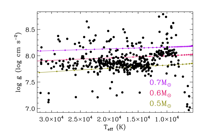
Figure 9.— Distribution of $T_{\rm eff}$ versus log $g$ for 419 of our WDs. Spectroscopic parameters for all targets are from Koester et al. (2009b). Notice the abrupt increase in the mean log $g$ around 12000 K. We also plot cooling tracks from evolutionary models for 0.5, 0.6 and 0.7 M_⊙ WDs.

5.4. Thick Disk DAs

The kinematics of thick disk stars prohibit us from placing them in the same co-moving reference frame as thin disk stars. In Section 5.3.2, we show that the kinematical LSR described by Standard Solar Motion is a suitable choice of reference frame for the SPY thin disk WDs. As expected, using $v_{\rm app}$ of our thick disk targets corrected to that LSR (the reference frame suitable for the thin disk) give discrepant values for $\langle v_{\rm app}\rangle$ in opposite directions. Since our thick disk sample is small (26 targets), our $\langle v_{\rm app}\rangle$ uncertainties are too large to discern a suitable reference frame. If we correct by the average lag in rotational velocity of the thick disk with respect to the thin disk ($\sim 40$ km s^-1; Gilmore et al., 1989), then $\langle v_{\rm app}\rangle=32.90\pm 9.59$ km s^-1 for our thick disk sample. Individual $v_{\rm app}$ measurements are listed in Table 2. Using $\langle T_{\rm eff}\rangle=19960$ K, we find $\langle M\rangle=0.652^{+0.097}_{-0.119}$ M_⊙, which is evidence that the mean mass of thick disk DAs is the same as for thin disk DAs.

One should also notice that the dispersion of $v_{\rm app}$ (Column 5 of Table 3) is clearly larger than that for the thin disk DAs. Since the $v_{\rm app}$ distribution is a convolution of the true mass distribution and the random stellar velocity distribution, this is consistent with a larger velocity dispersion as expected for the thick disk population (Gilmore et al., 1989).

6. Discussion

6.1. The Log $g$ Upturn

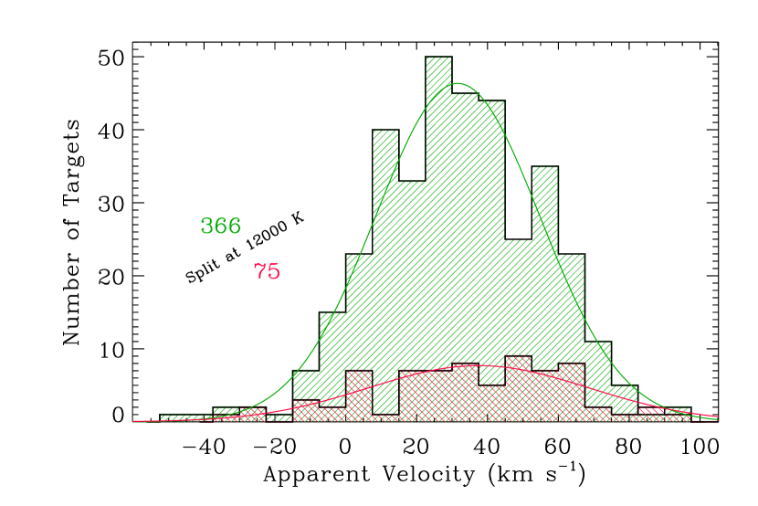
Figure 10.— Histogram of measured apparent velocities $v_{\rm app}$ for targets with spectroscopically determined $T_{\rm eff}$ from Koester et al. (2009b). The bin size is 7.5 km s^-1. The green histogram with ascending lines corresponds to targets with $T_{\rm eff}>12000$ K and the pink histogram with descending lines to $12000$ K $>T_{\rm eff}>7000$ K. The mean $v_{\rm app}$ for the green histogram is $31.61\pm 1.22$ km s^-1; the median is $31.71$ km s^-1; the standard deviation is $23.22$ km s^-1. The mean $v_{\rm app}$ for the pink histogram is $37.50\pm 3.59$ km s^-1; the median is $36.20$ km s^-1; the standard deviation is $31.00$ km s^-1. The overplotted curves are the Gaussian distribution functions used to determine Monte Carlo uncertainties. We list the number of targets in each distribution.

6.1.1 The Problem

A major problem plaguing the field of WDs is the apparent systematic increase in mean log $g$ for DAs toward low ($\lesssim 12,000$ K) $T_{\rm eff}$, as determined from spectroscopic fitting of absorption line profiles (Bergeron et al., 2007; Koester et al., 2009a). This increase is absent in photometric log $g$ determinations (Kepler et al., 2007; Engelbrecht & Koester, 2007), which are not strongly dependent on line profiles. A number of effects are known to exist that make theoretical line profile modeling for cool WD atmospheres more difficult than for hotter WDs, such as helium contamination from dredge-up (Bergeron et al., 1990; Tremblay & Bergeron, 2008) and the treatment of convective efficiency (Bergeron et al., 1995a). Neither of these, however, seem to solve the log $g$ upturn problem (Koester et al., 2009a), and since no strong hypotheses have been put forth to explain a real increase in mean mass (Kepler et al., 2007), the fault most likely lies with the atmosphere models or with the limitations of these models.

The number of studied cool WDs is already relatively low due to the inherent difficulty of observing cool objects, but the addition of the log $g$ upturn problem and the subtleties of cool WD atmosphere modeling has thus far kept that number low by prompting many spectroscopic analyses to be designed to exclude cooler WDs (e.g., Bergeron et al., 1992; Madej et al., 2004; Liebert et al., 2005; Kepler et al., 2007). This is tremendously unfortunate. Understanding cool WDs has broad astrophysical relevance, such as in determining the age of the Galactic disk (Winget et al., 1987) and in setting constraints on the physics of crystallization in high-density plasmas (Winget et al., 2009).

Furthermore, decades of focus on hotter WDs (due to the much larger dataset and due to the neglect of cooler WDs) have perhaps given researchers in our field a false comfort with these objects. There is a feeling that since hot WD atmospheres are more straightforward to model than cool atmospheres, the spectroscopic surface gravities (and masses) must be correct for the hot WDs and not for the cool WDs, given the log $g$ upturn problem. Recent improved calculations for Stark broadening of hydrogen lines in WD atmospheres (Tremblay & Bergeron, 2009) show that hot WD modeling is still maturing.

6.1.2 Avoiding the Upturn

The gravitational redshift method is independent of log $g$ determinations from atmosphere models and allows us to constrain changes in mean masses across $T_{\rm eff}$ bins.

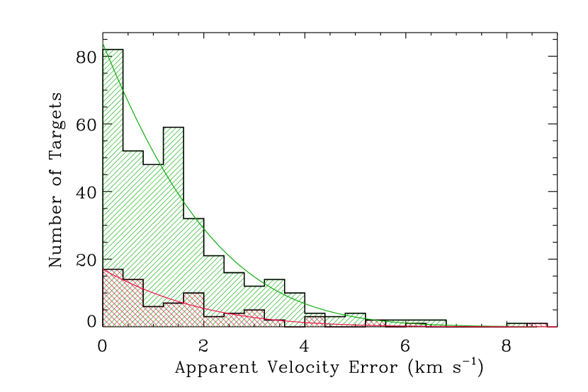
Figure 11.— Histogram of measured apparent velocities $v_{\rm app}$ for targets with spectroscopically determined $T_{\rm eff}$ from Koester et al. (2009b). The bin size is 7.5 km s^-1. The green histogram with ascending lines corresponds to targets with $T_{\rm eff}>12000$ K and the pink histogram with descending lines to $12000$ K $>T_{\rm eff}>7000$ K. The mean $v_{\rm app}$ for the green histogram is $31.61\pm 1.22$ km s^-1; the median is $31.71$ km s^-1; the standard deviation is $23.22$ km s^-1. The mean $v_{\rm app}$ for the pink histogram is $37.50\pm 3.59$ km s^-1; the median is $36.20$ km s^-1; the standard deviation is $31.00$ km s^-1. The overplotted curves are the Gaussian distribution functions used to determine Monte Carlo uncertainties. We list the number of targets in each distribution.

Figure 12.— Similar to Figure 5 but corresponding to targets with $T_{\rm eff}>12000$ K (green) and to targets with $12000$ K $>T_{\rm eff}>7000$ K (pink).

Figure 9 plots spectroscopically determined values of log $g$ and $T_{\rm eff}$ from Koester et al. (2009b) for the targets in our sample, clearly exposing the upturn. We plot evolutionary models for 0.5, 0.6 and 0.7 M_⊙ DA WDs to illustrate how a higher surface gravity implies a higher mass and to show the expected weak dependence on $T_{\rm eff}$. Using the mass-radius relation from evolutionary models, we derive mean spectroscopic masses $\langle M\rangle$ ${}^{\rm hot}=0.563\pm 0.002$ M_⊙ for 358 WDs with $T_{\rm eff}>12000$ K and $\langle M\rangle$ ${}^{\rm cool}=0.666\pm 0.005$ M_⊙ for 75 WDs with $12000$ K $>T_{\rm eff}>7000$ K; $\Delta\langle M\rangle=0.103\pm 0.007$ M_⊙. The mass difference is even larger in the SDSS data; Kepler et al. (2007) find $\langle M\rangle$ ${}^{\rm hot}=0.593\pm 0.016$ M_⊙ and $\langle M\rangle$ ${}^{\rm cool}=0.789\pm 0.005$ M_⊙ ($12000$ K $\geq T_{\rm eff}\geq 8500$ K); $\Delta\langle M\rangle=0.196\pm 0.021$ M_⊙.

In Figure 12, we show our distribution of $v_{\rm app}$ (distribution of uncertainties in Figure 12) for targets with $T_{\rm eff}>12000$ K (green histogram with ascending lines) and with $12000$ K $>T_{\rm eff}>7000$ K (pink histogram with descending lines). The corresponding $\langle v_{\rm app}\rangle$ determinations are $31.61\pm 1.22$ and $37.50\pm 3.59$ km s^-1, respectively, which translates to $\langle M\rangle$ ${}^{\rm hot}=0.640\pm 0.014$ M_⊙ and $\langle M\rangle$ ${}^{\rm cool}=0.686^{+0.035}_{-0.039}$ M_⊙ (see Figure 13). This is consistent with no change in mean mass across a temperature split at $T_{\rm eff}=12000$ K in agreement with the photometric studies by Kepler et al. (2007) and by Engelbrecht & Koester (2007). No previous large spectroscopic study has seen consistency in mean mass across these temperatures.

6.2. Comparison With Previous Studies

Table 5 lists four studies that employ the gravitational redshift method to determine masses for common proper motion WDs. Because of the small sample sizes (9, 35, 34, and 41 WDs), the uncertainties of the mean masses found by these studies are relatively large $-$ too large to discern a difference in mean mass from that of the spectroscopic method (Silvestri et al., 2001). Other than with the results of Koester (1987), whose sample consisted of only 9 DAs, our mean mass agrees with that of all these studies, and we improve upon the uncertainties (precision) by more than a factor of two.

The mean mass of 512 SPY non-binary thin disk normal DAs from Koester et al. (2009b), as we figure from their spectroscopically determined values of log $g$ and $T_{\rm eff}$, is $0.580\pm 0.002$ M_⊙, and if we restrict the comparison to 441 WDs in our sample, $\langle M\rangle$ $=0.575\pm 0.002$ M_⊙. Both values are significantly smaller than the mean mass we derive using the gravitational redshift method.

Using atmosphere models that implement the new Stark broadened line profiles from Tremblay & Bergeron (2009) and an updated treatment of the microfield distribution, the SPY sample shows an increase of $\sim 0.03$ M_⊙ in the mean mass (Koester, private communication), but this resulting mean mass is still significantly less than our value. In fact, our mean mass is significantly larger than the determinations from all the previous spectroscopic studies listed in Table 5 except that of Tremblay & Bergeron (2009).

The recent work of Tremblay & Bergeron (2009) uses atmosphere models with improved Stark broadening calculations to reanalyze the WDs from Liebert et al. (2005). They find a larger mean mass (0.649 M_⊙) than previously determined for the Palomar-Green sample (0.603 M_⊙). The mean mass we derive using the gravitational redshift method agrees well, thus providing independent observational evidence in support of these improved atmosphere models.

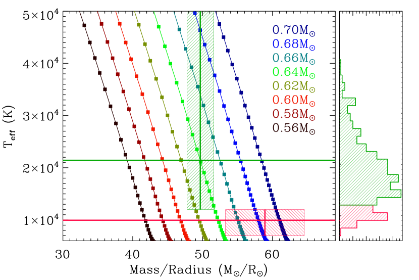
Figure 13.— Same as Figure 7 but for targets with $T_{\rm eff}>12000$ K (green) and with $12000$ K $>T_{\rm eff}>7000$ K (pink). $\langle M\rangle$ ${}^{\rm hot}=0.640\pm 0.014$ M_⊙ and $\langle M\rangle$ ${}^{\rm cool}=0.686^{+0.035}_{-0.039}$ M_⊙.

7. Conclusions

We show that the gravitational redshift method can be used to determine a mean mass of a sample of WDs whose dynamics are dominated by random stellar motions. For 449 non-binary thin disk normal DA WDs from SPY, we find $\langle v_{\rm g}\rangle=\langle v_{\rm app}\rangle=32.57\pm 1.16$ km s^-1. Using the mass-radius relation from evolutionary models, $\langle M\rangle=0.647^{+0.013}_{-0.014}$ M_⊙. This is in agreement with the results of previous gravitational redshift studies, but it is significantly higher than all previous spectroscopic determinations except that of Tremblay & Bergeron (2009).

We find that the targets in our sample move with respect to the kinematical LSR described by Standard Solar Motion (Kerr & Lynden-Bell, 1986) with the following values: ($U,V,W$)=($-1.62\pm 3.35,+1.84\pm 3.43,-1.67\pm 3.37$) km s^-1. This is consistent with no movement relative to this LSR.

Our results provide evidence that the mean mass of thick disk DAs is the same as for thin disk DAs.

The gravitational redshift method is independent of spectroscopically determined surface gravity from atmosphere models and is insensitive to the log $g$ upturn problem (Section 6.1). $\langle v_{\rm app}\rangle=31.61\pm 1.22$ and $37.50\pm 3.59$ km s^-1 for targets with $T_{\rm eff}>12000$ K and with $12000$ K $>T_{\rm eff}>7000$ K, respectively. This translates to $\langle M\rangle$ ${}^{\rm hot}=0.640\pm 0.014$ M_⊙ and $\langle M\rangle$ ${}^{\rm cool}=0.686^{+0.035}_{-0.039}$ M_⊙, which disagrees with spectroscopic results by showing no significant change in the mean mass of DAs across a temperature split at $T_{\rm eff}=12000$ K. This confirms the resuls of Kepler et al. (2007) and Engelbrecht & Koester (2007), who find no log $g$ increase in their photometric investigations. We are currently obtaining more observations of cool WDs to increase our sample size and hence precision of our mean mass determinations.

Table 1Apparent Velocity Measurements for Normal DA WDs (Abbreviated)

	Adopted				LSR	H$\alpha$			H$\beta$			Observation
	$v_{\rm app}$	$\delta v_{\rm app}$	Date	Time	Correction	$v_{\rm app}$	$\delta v_{\rm app}$		$v_{\rm app}$	$\delta v_{\rm app}$		$v_{\rm app}$	$\delta v_{\rm app}$
Target	(km s-1)	(km s-1)	(UT)	(UT)	(km s-1)	(km s-1)	(km s-1)		(km s-1)	(km s-1)		(km s-1)	(km s-1)
WD 0000-186	24.530	0.015	2000.09.16	04:53:07	-3.511	24.515	1.267		24.696	4.013		24.531	0.073
			2000.09.17	03:27:31	-3.825	24.190	0.742		29.329	4.231		24.343	1.236
HS 0002+1635	23.518	2.450	2002.12.02	01:07:24	-22.829	23.518	2.450		$\cdots$	$\cdots$		23.518	2.450
WD 0005-163	15.006	0.005	2000.09.16	03:31:59	-2.013	15.057	1.892		14.814	3.648		15.006	0.140
			2002.08.04	10:00:19	16.515	15.921	1.860		9.051	4.473		14.907	3.445
WD 0011+000	25.655	0.106	2000.07.14	07:14:10	28.209	23.079	0.949		20.950	2.568		22.823	0.978
			2000.07.17	07:38:21	27.631	25.660	0.657		25.542	4.107		25.657	0.025
WD 0013-241	15.760	0.061	2000.09.16	02:44:05	-3.848	15.754	1.063		15.797	2.591		15.760	0.020
			2000.09.17	01:52:24	-4.237	13.188	1.268		10.630	2.367		12.617	1.505
WD 0016-258	44.969	1.523	2000.09.16	03:01:00	-4.332	45.801	1.451		$\cdots$	$\cdots$		45.801	1.451
			2000.09.17	02:09:57	-4.713	44.016	2.194		39.586	6.581		43.573	1.879
WD 0016-220	10.875	1.715	2000.09.16	05:11:37	-2.989	12.101	0.868		16.054	1.894		12.788	2.117
			2000.09.17	03:47:05	-3.294	10.506	0.742		7.857	1.757		10.105	1.343
WD 0017+061	-1.247	3.824	2002.09.26	07:34:49	2.674	-0.139	2.876		-7.848	7.022		-1.247	3.824
WD 0018-339	30.744	0.565	2002.09.15	02:14:27	-6.478	31.118	1.042		29.443	2.256		30.823	0.901
			2002.09.18	02:33:07	-7.790	30.220	1.117		21.817	2.406		28.729	4.539
WD 0024-556	84.029	2.130	2000.08.03	09:18:35	-1.148	84.420	1.490		78.216	5.749		84.029	2.130
WD 0029-181	42.792	0.136	2002.09.26	08:24:34	-4.938	40.163	1.568		46.906	1.747		43.170	4.740
			2002.09.27	06:13:41	-5.196	42.249	1.494		44.187	2.475		42.767	1.212
HE 0031-5525	39.229	6.206	2001.12.17	00:53:54	-25.943	37.092	1.627		$\cdots$	$\cdots$		37.092	1.627
			2002.07.27	06:08:08	1.501	49.230	1.699		42.597	4.058		48.241	3.342
HE 0032-2744	48.911	3.650	2002.09.15	02:59:55	-2.771	51.692	2.379		$\cdots$	$\cdots$		51.692	2.379
			2002.09.18	03:06:41	-4.129	46.515	2.208		$\cdots$	$\cdots$		46.515	2.208
WD 0032-175	31.342	1.349	2002.09.18	03:21:03	-0.053	30.550	0.995		$\cdots$	$\cdots$		30.550	0.995
			2002.09.25	06:31:34	-3.823	32.492	1.200		$\cdots$	$\cdots$		32.492	1.200
WD 0032-177	9.875	3.692	2002.09.18	03:29:57	-0.101	10.312	1.452		6.331	1.284		8.078	2.793
			2002.09.25	06:01:55	-3.790	15.685	1.756		9.583	2.500		13.668	4.059
WD 0033+016	88.746	2.451	2002.09.26	07:57:13	2.732	88.746	2.451		$\cdots$	$\cdots$		88.746	2.451
MCT 0033-3440	47.910	0.286	2000.09.16	04:36:44	-6.179	52.870	1.751		$\cdots$	$\cdots$		52.870	1.751
			2002.08.15	09:54:03	6.272	47.879	1.316		48.012	2.860		47.902	0.071
HE 0043-0318	67.616	1.591	2002.12.02	01:30:55	-26.459	68.302	0.967		70.191	2.082		68.637	1.020
			2003.01.16	01:44:09	-29.463	66.376	1.124		$\cdots$	$\cdots$		66.376	1.124
WD 0047-524	23.980	0.368	2002.07.27	06:21:40	3.620	24.533	0.795		22.385	1.627		24.119	1.198
			2002.09.14	03:12:24	-10.877	24.175	0.716		19.757	1.671		23.488	2.263
HS 0047+1903	27.280	0.926	2002.09.27	05:30:35	10.719	27.042	1.183		29.084	3.262		27.280	0.926
WD 0048-544	22.199	0.822	2002.07.27	06:30:11	2.495	22.080	1.035		26.192	2.158		22.850	2.268
			2002.09.14	03:21:12	-11.578	23.188	0.995		20.319	0.944		21.679	2.026
WD 0048+202	35.980	0.587	2002.09.19	04:52:42	15.032	34.901	2.313		36.145	1.517		35.771	0.807
			2002.09.27	05:16:50	11.230	36.496	1.197		39.764	2.555		37.085	1.776
			2002.12.02	02:09:09	-18.947	36.612	1.150		31.783	2.525		35.783	2.575
HE 0049-0940	27.763	0.192	2002.09.26	08:39:23	0.509	27.896	1.001		26.624	2.178		27.675	0.682
			2002.09.27	06:27:15	0.251	28.308	0.783		26.327	1.736		27.973	1.049
WD 0050-332	35.597	1.801	2002.07.27	06:44:31	14.143	35.763	4.027		36.931	5.721		36.150	0.777
			2002.09.15	03:26:56	-3.174	31.345	2.874		$\cdots$	$\cdots$		31.345	2.874
			2002.09.25	06:49:51	-7.716	32.107	2.952		$\cdots$	$\cdots$		32.107	2.952
WD 0052-147	56.344	1.331	2002.09.26	08:54:09	-1.164	58.289	1.884		$\cdots$	$\cdots$		58.289	1.884
			2002.09.27	06:41:44	-1.422	56.297	2.405		54.873	3.785		55.888	0.912

Table 2Apparent Velocity Measurements for Thick Disk DAs

	Adopted				LSR	H$\alpha$			H$\beta$			Observation
	$v_{\rm app}$	$\delta v_{\rm app}$	Date	Time	Correction	$v_{\rm app}$	$\delta v_{\rm app}$		$v_{\rm app}$	$\delta v_{\rm app}$		$v_{\rm app}$	$\delta v_{\rm app}$
Target	(km s-1)	(km s-1)	(UT)	(UT)	(km s-1)	(km s-1)	(km s-1)		(km s-1)	(km s-1)		(km s-1)	(km s-1)
WD 0158-227	-12.279	2.795	2002.09.20	03:40:17	-5.823	-10.305	1.125		$\cdots$	$\cdots$		-10.305	1.125
			2002.09.27	07:46:45	-9.161	-14.259	1.127		$\cdots$	$\cdots$		-14.259	1.127
WD 0204-233	82.384	0.304	2000.07.15	07:45:18	8.895	82.192	0.944		80.422	1.662		81.760	1.074
			2000.07.17	08:47:06	8.750	82.364	1.977		83.186	5.477		82.459	0.371
WD 0255-705	47.623	0.527	2000.08.03	09:55:52	-35.536	48.181	1.547		$\cdots$	$\cdots$		48.181	1.547
			2000.08.05	08:51:01	-35.778	47.374	1.034		$\cdots$	$\cdots$		7.374	1.034
WD 0352+052	-86.636	2.300	2002.03.01	01:09:46	-35.737	-87.408	1.401		$\cdots$	$\cdots$		-87.408	1.401
			2002.09.13	09:27:33	19.231	-84.384	1.248		-79.498	2.216		-83.208	2.954
HE 0409-5154	23.915	6.616	2000.09.15	09:10:28	-37.306	22.243	2.047		20.299	1.634		21.056	1.340
			2001.09.13	09:26:42	-37.020	30.762	1.257		34.543	2.406		31.572	2.194
HE 0416-1034	44.087	0.191	2000.12.17	06:13:24	-38.231	43.785	1.509		45.786	3.788		44.059	0.973
			2001.01.15	03:03:25	-48.043	40.481	2.058		47.436	1.631		44.754	4.787
HE 0452-3444	-10.387	0.086	2000.12.13	06:27:39	-44.215	-9.733	1.464		-13.936	3.554		-10.343	2.094
			2001.01.15	02:44:23	-51.955	-9.238	2.210		-13.956	3.712		-10.472	2.932
HE 0508-2343	79.982	2.028	2001.04.07	00:23:02	-59.490	79.124	1.786		80.903	1.307		80.283	1.198
			2001.04.09	00:48:48	-59.118	76.884	1.817		68.789	1.966		73.155	5.706
WD 0732-427	36.295	0.558	2001.04.09	01:16:13	-68.414	36.003	0.756		37.866	1.433		36.409	1.087
			2001.05.03	23:55:10	-69.286	33.730	1.190		40.950	2.679		34.920	3.788
HS 0820+2503	41.390	4.704	2003.02.18	02:42:33	-33.578	41.390	4.704		$\cdots$	$\cdots$		41.390	4.704
HE 1124+0144	46.460	0.144	2000.07.01	23:28:45	-55.699	45.879	1.394		48.423	2.799		46.384	1.435
			2000.07.02	23:34:25	-55.550	47.083	1.185		42.748	3.337		46.598	1.932
WD 1152-287	51.828	1.745	2000.07.11	00:57:00	-70.466	50.760	1.594		$\cdots$	$\cdots$		50.760	1.594
			2000.07.14	23:01:27	-70.053	53.254	1.841		$\cdots$	$\cdots$		53.254	1.841
WD 1323-514	-40.353	0.770	2001.05.15	01:29:38	-42.147	-40.093	0.793		-41.065	2.400		-40.189	0.409
			2001.06.08	02:12:18	-50.778	-42.707	1.018		-40.445	1.821		-42.168	1.362
WD 1334-678	22.946	0.649	2000.07.30	00:47:19	-58.211	22.384	1.473		24.018	3.072		22.689	0.900
			2001.05.15	01:42:37	-40.116	24.128	1.309		20.157	4.143		23.767	1.612
HS 1338+0807	64.191	2.405	2001.08.18	23:52:07	-28.395	64.191	2.405		$\cdots$	$\cdots$		64.191	2.405
WD 1410+168	15.184	2.748	2002.04.23	06:08:33	7.586	15.753	0.911		8.557	3.107		15.184	2.748
WD 1426-276	55.800	0.559	2000.07.05	03:56:09	-43.083	55.742	1.182		55.448	3.136		55.705	0.137
			2000.07.06	02:38:26	-43.227	57.693	1.045		56.772	1.755		57.452	0.572
HS 1432+1441	84.966	3.366	2001.08.16	00:01:42	-14.425	82.686	1.642		77.964	3.260		81.730	2.683
			2001.08.21	00:15:53	-13.555	85.505	1.995		88.323	2.297		86.717	1.973
WD 1507+021	50.907	3.076	2002.06.18	01:25:19	-7.271	52.338	2.198		47.601	3.340		50.907	3.076
WD 1614-128	95.682	0.052	2000.06.06	06:16:38	5.840	94.870	1.239		99.368	2.581		95.713	2.482
			2000.06.08	02:20:56	5.346	94.931	1.088		102.053	3.282		95.637	3.009
WD 1716+020	10.643	1.291	2002.04.23	09:03:16	48.550	11.038	0.846		8.531	1.956		10.643	1.291
WD 1834-781	60.781	0.111	2000.07.06	04:36:43	-35.096	60.857	0.919		60.355	2.395		60.792	0.237
			2000.07.13	05:04:33	-37.059	59.611	1.028		62.217	1.793		60.255	1.589
WD 1952-206	62.701	0.113	2000.07.06	05:09:15	29.248	62.167	0.870		63.309	2.141		62.329	0.563
			2000.07.13	04:43:35	25.831	62.683	0.956		62.931	2.356		62.718	0.122
WD 2029+183	-97.198	1.373	2002.04.24	09:34:58	74.163	-98.949	2.029		-96.770	1.646		-97.635	1.507
			2002.08.05	04:50:45	51.952	-93.455	1.652		-98.577	2.467		-95.041	3.349
WD 2322-181	39.763	1.328	2000.07.13	06:16:26	38.666	42.172	1.462		38.142	2.548		41.173	2.459
			2000.07.16	05:46:18	37.813	39.731	1.648		36.877	3.217		39.138	1.638
WD 2350-083	84.801	0.992	2002.07.11	09:56:33	49.133	84.652	1.390		85.845	2.341		84.963	0.740
			2002.09.13	07:51:37	24.339	80.737	1.489		86.827	3.323		81.756	3.214

Table 3Mean Apparent Velocities

		$\langle v_{\rm app}\rangle$	$\delta\langle v_{\rm app}\rangle$	$\sigma_{v_{\rm app}}$	$\langle\delta$$v_{\rm app}\rangle$	$\langle M/R\rangle$	$\delta\langle M/R\rangle$
Sample	# of WDs	(km s-1)	(km s-1)	(km s-1)	(km s-1)	(M⊙/R⊙)	(M⊙/R⊙)
Main	449	32.57	1.17	24.84	1.51	51.19	1.84
H$\alpha$	449	32.69	1.18	24.87	1.78	51.37	1.85
H$\beta$	372	31.47	1.32	25.52	3.17	49.45	2.07
Thick	26	32.90	9.59	48.99	1.57	51.70	15.07

Table 4Mean Masses

		$\langle v_{\rm app}\rangle$	$\delta$ $\langle v_{\rm app}\rangle$	$\langle T_{\rm eff}\rangle$	$\sigma_{T_{\rm eff}}$	$\langle M\rangle$	$\delta$ $\langle M\rangle$
Sample	# of WDs	(km s-1)	(km s-1)	(K)	(K)	(M⊙)	(M⊙)
Main	449	32.57	1.17	19400	9950	0.647	${}^{+0.013}_{-0.014}$
Thick	26	32.90	9.59	19960	11060	0.652	${}^{+0.097}_{-0.119}$
Hot	366	31.61	1.22	21670	9700	0.640	0.014
Cool	75	37.50	3.59	9950	1090	0.686	${}^{+0.035}_{-0.039}$

Table 5Mean DA Masses From Selected Previous Studies

		$\langle M\rangle$	$\delta$ $\langle M\rangle$	$\sigma_{M}$		Assumed
Study	# of WDs	(M⊙)	(M⊙)	(M⊙)	Method	H-Layer	Notes
Koester et al. (1979)	122	0.58	0.10	0.12	Photo	Thin/No
Koester (1987)	9	0.58	$\cdots$	0.11	GRS	Thin/No	CPM WDs
McMahan (1989)	50	0.523	0.014	$\cdots$	Spectro	Thin/No
Wegner & Reid (1991)	35	0.63	0.03	$\cdots$	GRS	Thin/No	CPM WDs
Bergeron et al. (1992)	129	0.562	$\cdots$	0.137	Spectro	Thin/No	$T_{\rm eff}\gtrsim 14000$ K
Bragaglia et al. (1995)	42	0.609	$\cdots$	0.157	Spectro	Thin/No	$T_{\rm eff}>12000$ K
Bergeron et al. (1995b)	129	0.590	$\cdots$	0.134	Spectro	Thick	Revised Bergeron et al. (1992)
							w/ thick H-layers
Reid (1996)	34	0.583	0.078	$\cdots$	GRS	Thick	CPM WDs
Vennes et al. (1997)	110	0.56*	$\cdots$	$\cdots$	Spectro	Thin/No	$75000$ K $\gtrsim T_{\rm eff}\gtrsim 25000$ K
Finley et al. (1997)	174	0.570*	$\cdots$	0.060*	Spectro	Thick	$T_{\rm eff}\gtrsim 25000$ K
							some w/ cool companions
Silvestri et al. (2001)	41	0.68	0.04	$\cdots$	GRS	Thick	CPM WDs
Madej et al. (2004)	1175	0.562*	$\cdots$	$\cdots$	Spectro	Thick	$T_{\rm eff}\geq 12000$ K
Liebert et al. (2005)	298	0.603	$\cdots$	0.134	Spectro	Thick	$T_{\rm eff}>13000$ K
		0.572*	$\cdots$	0.188
Kepler et al. (2007)	1859	0.593	0.016	$\cdots$	Spectro	Thick	$T_{\rm eff}>12000$ K
Tremblay & Bergeron (2009)	$\sim 250$	0.649	$\cdots$	$\cdots$	Spectro	Thick	$40000$ K $>T_{\rm eff}>12000$ K
							overlap w/ Liebert et al.
Koester et al. (2009b)	606	0.567	0.002	0.142	Spectro	Thick	SPY
Koester et al. (2009b)	512	0.580	0.002	0.136			SPY non-binary thin disk WDs
Koester et al. (2009b) overlap	441	0.575	0.002	0.128
This Work	449	0.647	${}^{+0.013}_{-0.014}$	$\cdots$	GRS	Thick	SPY non-binary thin disk WDs

Note. — Masses marked with an asterisk are peaks/widths of mass distributions from Gaussian fitting.

References

- Althaus & Benvenuto (1998) Althaus, L. G., & Benvenuto, O. G. 1998, MNRAS, 296, 206
- Althaus et al. (2002) Althaus, L. G., Serenelli, A. M., Córsico, A. H., & Benvenuto, O. G. 2002, MNRAS, 330, 685
- Bergeron et al. (2007) Bergeron, P., Gianninas, A., & Boudreault, S. 2007, in Astronomical Society of the Pacific Conference Series, Vol. 372, 15th European Workshop on White Dwarfs, ed. R. Napiwotzki & M. R. Burleigh, 29–+
- Bergeron et al. (1995a) Bergeron, P., Liebert, J., & Fulbright, M. S. 1995a, ApJ, 444, 810
- Bergeron et al. (1992) Bergeron, P., Saffer, R. A., & Liebert, J. 1992, ApJ, 394, 228
- Bergeron et al. (1990) Bergeron, P., Wesemael, F., Fontaine, G., & Liebert, J. 1990, ApJ, 351, L21
- Bergeron et al. (1995b) Bergeron, P., Wesemael, F., Lamontagne, R., Fontaine, G., Saffer, R. A., & Allard, N. F. 1995b, ApJ, 449, 258
- Bischoff-Kim et al. (2008) Bischoff-Kim, A., Montgomery, M. H., & Winget, D. E. 2008, ApJ, 675, 1505
- Bragaglia et al. (1995) Bragaglia, A., Renzini, A., & Bergeron, P. 1995, ApJ, 443, 735
- Castanheira & Kepler (2009) Castanheira, B. G., & Kepler, S. O. 2009, MNRAS, 396, 1709
- Chandrasekhar (1939) Chandrasekhar, S. 1939, An Introduction to the Study of Stellar Structure, ed. S. Chandrasekhar (The University of Chicago Press)
- Christlieb et al. (2001) Christlieb, N., Wisotzki, L., Reimers, D., Homeier, D., Koester, D., & Heber, U. 2001, A&A, 366, 898
- DeGennaro et al. (2008) DeGennaro, S., von Hippel, T., Winget, D. E., Kepler, S. O., Nitta, A., Koester, D., & Althaus, L. 2008, AJ, 135, 1
- Dekker et al. (2000) Dekker, H., D’Odorico, S., Kaufer, A., Delabre, B., & Kotzlowski, H. 2000, in Society of Photo-Optical Instrumentation Engineers (SPIE) Conference Series, Vol. 4008, Society of Photo-Optical Instrumentation Engineers (SPIE) Conference Series, ed. M. Iye & A. F. Moorwood, 534–545
- Engelbrecht & Koester (2007) Engelbrecht, A., & Koester, D. 2007, in Astronomical Society of the Pacific Conference Series, Vol. 372, 15th European Workshop on White Dwarfs, ed. R. Napiwotzki & M. R. Burleigh, 289–+
- Fich et al. (1989) Fich, M., Blitz, L., & Stark, A. A. 1989, ApJ, 342, 272
- Finley & Koester (1997) Finley, D. S., & Koester, D. 1997, ApJ, 489, L79+
- Finley et al. (1997) Finley, D. S., Koester, D., & Basri, G. 1997, ApJ, 488, 375
- Fontaine et al. (1985) Fontaine, G., Bergeron, P., Lacombe, P., Lamontagne, R., & Talon, A. 1985, AJ, 90, 1094
- Fontaine & Wesemael (1997) Fontaine, G., & Wesemael, F. 1997, in Astrophysics and Space Science Library, Vol. 214, White dwarfs, ed. J. Isern, M. Hernanz, & E. Garcia-Berro, 173–+
- Gatewood & Gatewood (1978) Gatewood, G. D., & Gatewood, C. V. 1978, ApJ, 225, 191
- Gilmore et al. (1989) Gilmore, G., Wyse, R. F. G., & Kuijken, K. 1989, ARA&A, 27, 555
- Girardi et al. (2000) Girardi, L., Bressan, A., Bertelli, G., & Chiosi, C. 2000, A&AS, 141, 371
- Grabowski et al. (1987) Grabowski, B., Halenka, J., & Madej, J. 1987, ApJ, 313, 750
- Greenstein & Trimble (1967) Greenstein, J. L., & Trimble, V. L. 1967, ApJ, 149, 283
- Hagen et al. (1995) Hagen, H.-J., Groote, D., Engels, D., & Reimers, D. 1995, A&AS, 111, 195
- Homeier et al. (1998) Homeier, D., Koester, D., Hagen, H.-J., Jordan, S., Heber, U., Engels, D., Reimers, D., & Dreizler, S. 1998, A&A, 338, 563
- Jordan et al. (1998) Jordan, S., Koester, D., Vauclair, G., Dolez, N., Heber, U., Hagen, H.-J., Reimers, D., Chevreton, M., & Dreizler, S. 1998, A&A, 330, 277
- Kepler et al. (2007) Kepler, S. O., Kleinman, S. J., Nitta, A., Koester, D., Castanheira, B. G., Giovannini, O., Costa, A. F. M., & Althaus, L. 2007, MNRAS, 375, 1315
- Kerr & Lynden-Bell (1986) Kerr, F. J., & Lynden-Bell, D. 1986, MNRAS, 221, 1023
- Kilic et al. (2008) Kilic, M., Thorstensen, J. R., & Koester, D. 2008, ApJ, 689, L45
- Kilkenny et al. (1997) Kilkenny, D., O’Donoghue, D., Koen, C., Stobie, R. S., & Chen, A. 1997, MNRAS, 287, 867
- Koester (1987) Koester, D. 1987, ApJ, 322, 852
- Koester et al. (2009a) Koester, D., Kepler, S. O., Kleinman, S. J., & Nitta, A. 2009a, Journal of Physics Conference Series, 172, 012006
- Koester et al. (2001) Koester, D., Napiwotzki, R., Christlieb, N., Drechsel, H., Hagen, H.-J., Heber, U., Homeier, D., Karl, C., Leibundgut, B., Moehler, S., Nelemans, G., Pauli, E.-M., Reimers, D., Renzini, A., & Yungelson, L. 2001, A&A, 378, 556
- Koester et al. (1979) Koester, D., Schulz, H., & Weidemann, V. 1979, A&A, 76, 262
- Koester et al. (2009b) Koester, D., Voss, B., Napiwotzki, R., Christlieb, N., Homeier, D., Lisker, T., Reimers, D., & Heber, U. 2009b, A&A, 505, 441
- Kuijken & Gilmore (1989) Kuijken, K., & Gilmore, G. 1989, MNRAS, 239, 605
- Lamontagne et al. (2000) Lamontagne, R., Demers, S., Wesemael, F., Fontaine, G., & Irwin, M. J. 2000, AJ, 119, 241
- Lawlor & MacDonald (2006) Lawlor, T. M., & MacDonald, J. 2006, MNRAS, 371, 263
- Liebert et al. (2005) Liebert, J., Bergeron, P., & Holberg, J. B. 2005, ApJS, 156, 47
- Madej et al. (2004) Madej, J., Należyty, M., & Althaus, L. G. 2004, A&A, 419, L5
- Maxted & Marsh (1999) Maxted, P. F. L., & Marsh, T. R. 1999, MNRAS, 307, 122
- Maxted et al. (2000) Maxted, P. F. L., Marsh, T. R., & Moran, C. K. J. 2000, MNRAS, 319, 305
- McCook & Sion (1999) McCook, G. P., & Sion, E. M. 1999, ApJS, 121, 1
- McMahan (1989) McMahan, R. K. 1989, ApJ, 336, 409
- Mestel (1952) Mestel, L. 1952, MNRAS, 112, 583
- Montgomery et al. (1999) Montgomery, M. H., Klumpe, E. W., Winget, D. E., & Wood, M. A. 1999, ApJ, 525, 482
- Napiwotzki (2009) Napiwotzki, R. 2009, Journal of Physics Conference Series, 172, 012004
- Napiwotzki et al. (2003) Napiwotzki, R., Christlieb, N., Drechsel, H., Hagen, H., Heber, U., Homeier, D., Karl, C., Koester, D., Leibundgut, B., Marsh, T. R., Moehler, S., Nelemans, G., Pauli, E., Reimers, D., Renzini, A., & Yungelson, L. 2003, The Messenger, 112, 25
- Napiwotzki et al. (2001) Napiwotzki, R., Christlieb, N., Drechsel, H., Hagen, H.-J., Heber, U., Homeier, D., Karl, C., Koester, D., Leibundgut, B., Marsh, T. R., Moehler, S., Nelemans, G., Pauli, E.-M., Reimers, D., Renzini, A., & Yungelson, L. 2001, Astronomische Nachrichten, 322, 411
- Pauli et al. (2006) Pauli, E.-M., Napiwotzki, R., Heber, U., Altmann, M., & Odenkirchen, M. 2006, A&A, 447, 173
- Reid (1996) Reid, I. N. 1996, AJ, 111, 2000
- Richter et al. (2007) Richter, R., Heber, U., & Napiwotzki, R. 2007, in Astronomical Society of the Pacific Conference Series, Vol. 372, 15th European Workshop on White Dwarfs, ed. R. Napiwotzki & M. R. Burleigh, 107–+
- Shipman (1979) Shipman, H. L. 1979, ApJ, 228, 240
- Shipman & Mehan (1976) Shipman, H. L., & Mehan, R. G. 1976, ApJ, 209, 205
- Shipman & Sass (1980) Shipman, H. L., & Sass, C. A. 1980, ApJ, 235, 177
- Silvestri et al. (2001) Silvestri, N. M., Oswalt, T. D., Wood, M. A., Smith, J. A., Reid, I. N., & Sion, E. M. 2001, AJ, 121, 503
- Sion et al. (2009) Sion, E. M., Holberg, J. B., Oswalt, T. D., McCook, G. P., & Wasatonic, R. 2009, AJ, 138, 1681
- Tremblay & Bergeron (2008) Tremblay, P.-E., & Bergeron, P. 2008, ApJ, 672, 1144