Viscosity of strongly interacting quantum fluids: spectral functions and sum rules

Abstract

The viscosity of strongly interacting systems is a topic of great interest in diverse fields. We focus here on the bulk and shear viscosities of non-relativistic quantum fluids, with particular emphasis on strongly interacting ultracold Fermi gases. We use Kubo formulas for the bulk and shear viscosity spectral functions, $\zeta(\omega)$ and $\eta(\omega)$ respectively, to derive exact, non-perturbative results. Our results include: a microscopic connection between the shear viscosity $\eta$ and the normal fluid density $\rho_{n}$; sum rules for $\zeta(\omega)$ and $\eta(\omega)$ and their evolution through the BCS-BEC crossover; universal high-frequency tails for $\eta(\omega)$ and the dynamic structure factor $S({\bf q},\omega)$. We use our sum rules to show that, at unitarity, $\zeta(\omega)$ is identically zero and thus relate $\eta(\omega)$ to density-density correlations. We predict that frequency-dependent shear viscosity $\eta(\omega)$ of the unitary Fermi gas can be experimentally measured using Bragg spectroscopy.

I Introduction

The study of the viscosity of strongly interacting quantum fluids has brought together very different areas of physics – black holes and string theory, quark-gluon plasmas, quantum fluids and cold atoms – which, at first sight, appear to have little in common Son-review ; Schafer09 . This extraordinary development originated with the work of Son, Starinets and coworkers Son-review ; Policastro01 ; Kovtun05 who calculated the shear viscosity in a strongly interacting quantum field theory, the ${\cal{N}}=4$ supersymmetric Yang-Mills (SYM) theory, and conjectured a lower bound

$${\eta}/{s}\geq{\hbar}/{(4\pi k_{B})}$$ (1)

for the ratio of the shear viscosity $\eta$ to the entropy density $s$ of any system. These results were obtained using the AdS/CFT formalism where certain strongly coupled field theories can be mapped onto weakly coupled gravity theories.

Although a number of counterexamples have since been proposed Cohen07 ; Brigante08 ; Kats09 ; Buchel09 , there are no known experimental violations of the bound given by Eq. (1). Remarkably, two very different experimental systems come close to saturating the bound: the quark-gluon plasma at Brookhaven’s Relativistic Heavy Ion Collider RHIC ; Teaney01 , and ultracold atomic Fermi gases Turlapov08 ; Gelman05 close to a Feshbach scattering resonance, where the $s$-wave scattering length becomes infinite Trentoreview . This is the strongly interacting unitary regime that lies at the center of the BCS-BEC crossover. These two systems are amongst the hottest and coldest systems every realized in a laboratory.

In this paper we focus on non-relativistic quantum fluids, with particular emphasis on strongly interacting Fermi gases. These are systems for which the most controlled experiments should be possible. A “perfect fluid” with the minimum shear viscosity is necessarily in a quantum regime, since the bound involves $\hbar$. In addition, it must also be in a strongly interacting regime where well-defined quasiparticle excitations do not exist. If the system had sharp quasiparticles, then their mean scattering rate $\tau^{-1}$ would be much less than the average energy per particle $\epsilon_{0}$, so that $\hbar/\tau\ll\epsilon_{0}$. We can then use Boltzmann’s kinetic theory approach to obtain $\eta\sim n\epsilon_{0}\tau$, where $n$ is the number density. Using $s\sim nk_{B}$, we find a large $\eta/s\sim\epsilon_{0}\tau/k_{B}\gg{\hbar}/{k_{B}}$. Thus, in order to find perfect fluids that come close to saturating the lower bound given by Eq. (1), one must look at strongly interacting quantum fluids where the quasiparticle approximation fails.

In this paper we use Kubo formulas for the frequency-dependent spectral functions for shear viscosity $\eta(\omega)$ and bulk (or second) viscosity $\zeta(\omega)$, and derive several exact, non-perturbative results without making weak coupling or quasiparticle approximations. Our main results are:

$\bullet$ We establish a microscopic connection between the shear viscosity $\eta$ and the normal fluid density $\rho_{n}$ and show that a non-zero $\rho_{n}$ is a necessary condition for a non-vanishing $\eta$.

$\bullet$ We derive sum rules for $\eta(\omega)$ and $\zeta(\omega)$ of any Bose or Fermi system with an arbitrary two-body interaction; see Eqs. (52) and (53).

$\bullet$ For a dilute two-component Fermi gas, we find the shear viscosity sum rule

$$\frac{1}{\pi}\int^{\infty}_{0}\!\!d\omega\left[\eta(\omega)-\frac{C}{10\pi\sqrt{m\omega}}\right]=\frac{\varepsilon}{3}-\frac{C}{10\pi ma},$$ (2)

valid for arbitrary temperature and $1/(k_{F}a)$, where $a$ is the $s$-wave scattering length. Here, $\varepsilon$ is the energy density and $C$ is the contact Tan08 . A central quantity in many of our results, $C=k_{F}^{4}{\cal C}[1/(k_{F}a),T/\epsilon_{F}]$ can be defined via the large-$k$ tail of the momentum distribution $n_{{\bf k}}\simeq C/k^{4}$ for $k\gg k_{F}$, and characterizes the short-distance properties of the many-body state.

$\bullet$ For the bulk viscosity, we obtain the sum rule

$$\frac{1}{\pi}\int^{\infty}_{0}d\omega\;\zeta(\omega)=\frac{1}{72\pi ma^{2}}\left(\frac{\partial C}{\partial a^{-1}}\right)_{s},$$ (3)

where the derivative is at fixed entropy per particle $s\equiv S/N$. [Different from Eq. (1), in the remainder of this paper we use $s$ to denote this quantity rather than the entropy density.] Below the superfluid transition, the bulk viscosity that enters Eq. (3) is $\zeta_{2}$, associated with the damping of in-phase motions of the superfluid and normal components. The positivity of $\zeta(\omega)$ implies that $(\partial C/\partial a^{-1})_{s}\geq 0$.

$\bullet$ At unitarity, the bulk viscosity spectral function vanishes at all frequencies and all temperatures. Quite generally, $\zeta(\omega)\geq 0$, but the sum rule in Eq. (3) vanishes for $|a|=\infty$ and thus $\zeta(\omega)=0$ for the unitary Fermi gas. This generalizes the result Son07 that the static bulk viscosity $\zeta(0)$ vanishes at unitarity.

$\bullet$ It follows from the previous result that, at unitarity, the shear viscosity spectral function $\eta(\omega)$ can be related to density-density correlations as

$$\eta(\omega)=\lim_{q\to 0}\frac{3\omega^{3}}{4q^{4}}\;\mathrm{Im}\chi_{\rho\rho}({\bf q},\omega)\ \ \ \ \ (|a|=\infty).$$ (4)

Thus, $\eta(\omega)$ for the unitary Fermi gas can be measured spectroscopically using, for instance, two-photon Bragg spectroscopy.

$\bullet$ We show from our sum rules that various dynamic response functions for Fermi gases have high-frequency tails characterized by odd-integer power laws, whose magnitudes are controlled by the contact $C$. The tail $C/\sqrt{\omega}$ of $\eta(\omega)$ is evident from Eq. (2). Using this we find that the dynamic structure factor has a tail of the form Son10 $S({{\bf q}},\omega)\sim Cq^{4}/\omega^{7/2}$ for $q\to 0$ and $\omega\to\infty$, which is shown to be a generic feature of short range physics.

In the remainder of this Section we describe how the rest of the paper is organized. In Section II, we begin with a careful derivation of Kubo formulas for the spectral functions $\eta(\omega)$ and $\zeta(\omega)$ in terms of current-current correlation functions, Eqs. (20) and (21), and, equivalently, in terms of the stress-stress correlator, Eq. (28).

In Section III we recall some elementary facts about the shear viscosity of a fluid and why it is analogous to the resistivity, and not the conductivity, of a metal. We then establish a connection between the viscosity $\eta$ and the normal fluid density $\rho_{n}$ using microscopic response functions.

After establishing the positivity of $\eta(\omega)$ and of $\zeta(\omega)$ in Section IV, we derive sum rules for these quantities in Section V. The most general sum rules for the shear and bulk viscosities of any Bose or Fermi system with an arbitrary isotropic interaction potential $V(p)$, and valid for all temperatures, are given in Eqs. (52) and (53).

In Section VI, we specialize to the dilute Fermi gas, with interparticle spacing $k_{F}^{-1}$ and $s$-wave scattering length $a$ both much larger than the characteristic range $r_{0}$ of the potential. We obtain the $\zeta$ sum rule in Eq. (3), which is finite in the zero range limit. The $\eta$ sum rule, however, has an ultraviolet divergence; see Eq. (66). We identify, in Section VII, the $C/\sqrt{\omega}$ high-frequency tail of the shear viscosity spectral function, and derive the sum rule given by Eq. (2), which is manifestly finite for $r_{0}\to 0$. The sum rules given by Eqs. (2) and (3) are valid in both the normal and superfluid phases, with $\zeta$ replaced by $\zeta_{2}$ in the latter state.

In Section VIII we show from the $\zeta$ sum rule that, at unitarity, $\zeta(\omega)$ vanishes at all frequencies and all temperatures. We also discuss the $1/(k_{F}a)$-dependence of the $\eta$ and $\zeta$ sum rules across the BCS-BEC crossover, using available quantum Monte Carlo data for the energy density at $T=0$.

We discuss the connection between viscosity and density-density correlations in Section IX and find two interesting results. First, we show how a density probe such as two-photon Bragg spectroscopy can in principle be used to measure the shear viscosity spectral function $\eta(\omega)$ at unitarity. Second, we identify the high-frequency $\omega^{-7/2}$ tail in the dynamic structure factor $S({{\bf q}},\omega)$.

In Section X, we briefly compare the sum rules that we have derived for non-relativistic quantum fluids with those obtained in relativistic quantum field theories. Finally in Section XI we conclude with open questions.

There are five Appendices which contain technical details of derivations or review certain results which are used at various places in the paper. In Appendix A, we briefly discuss an alternate stress tensor operator often used to calculate the shear viscosity. Some results from dissipative two-fluid hydrodynamics, which we use in our paper, are reviewed in Appendix B. We review in Appendix C results related to the contact that are used at several places in the paper, and also give a detailed derivation of certain equations that involve the contact. In Appendix D, we derive a microscopic expression for the pressure. Finally, in Appendix E we give details of the derivation of the $\zeta$ sum rule which make use of the scaling form of thermodynamic functions across the BCS-BEC crossover.

II Kubo formula for viscosity

We begin by deriving Kubo formulas for the bulk and shear viscosity. Although the results of this Section are, for the most part, “well known”, we could not find a complete derivation at any one place in the literature. In particular, there are several subtle points not dealt with adequately elsewhere, not least the definition of the stress tensor operator $\widehat{\Pi}_{\alpha\beta}$ for non-relativistic systems.

To introduce notation, we start with the Euler equation

$$m\partial_{t}j_{\alpha}({\bf r},t)=-\partial_{\beta}\Pi_{\alpha\beta}({\bf r},t),$$ (5)

where $m$ is the mass of the particles, $j_{\alpha}$ is the (number) current and $\Pi_{\alpha\beta}$ is the momentum flux density tensor, which we call the stress tensor, for short. Here, $\alpha$ and $\beta$ take on values $x,y,z$ (and there is no difference between upper and lower indices in our non-relativistic formulation). In general, the stress tensor is given by LLFM

$$\Pi_{\alpha\beta}=P\delta_{\alpha\beta}+\rho u_{\alpha}u_{\beta}-\sigma^{\prime}_{\alpha\beta},$$ (6)

where $P$ is the pressure, $\rho$ the mass density and ${\bm{u}}$ the velocity. The viscous term $\sigma^{\prime}_{\alpha\beta}$ is given by

$$\sigma^{\prime}_{\alpha\beta}=\eta\left[\partial_{\beta}u_{\alpha}\!+\!\partial_{\alpha}u_{\beta}\!-\!\frac{2}{3}\delta_{\alpha\beta}({\bm{\nabla}}\cdot{\bm{u}})\right]\!+\!\zeta\delta_{\alpha\beta}({\bm{\nabla}}\cdot{\bm{u}}),$$ (7)

where $\eta$ is the shear viscosity and $\zeta$ the bulk viscosity. The generalization of Eq. (7) to the superfluid state is well known LLFM and involves additional bulk viscosities. At the end of Section II.1, we show that the Kubo formula we derive for $\zeta$ describes the bulk viscosity $\zeta_{2}$ in the superfluid phase.

Our goal is to obtain Kubo formulas for frequency-dependent generalizations of the long-wavelength viscosities, $\eta$ and $\zeta$, in terms of equilibrium correlation functions of the many-body system. The Kubo formulas for viscosities are often written in terms of the stress-stress correlators; see, e.g., Sec. 90 of Ref. LLStatPhysII . However, the form of the stress tensor (or momentum flux density) operator $\widehat{\Pi}_{\alpha\beta}$ is not obvious, and many different, complicated expressions Forster which are presumably equivalent can be found in the literature. Part of the problem is to write down an operator expression for the pressure $P$ in terms of particle positions and momenta. In high-energy physics, a simple way to calculate the stress-energy tensor $\widehat{\Pi}_{\alpha\beta}$ is to vary the action with respect to the metric in curved space-time. We prefer, however, to describe non-relativistic fluids without going to curved space-time.

To begin with, in II.1, we adopt an approach that permits us to get around the complexities of defining the stress operator $\widehat{\Pi}$. We consider the linear response of a fluid to an externally imposed velocity field and derive Kubo formulas for the bulk and shear viscosities in terms of current-current correlators. The results of this subsection are the same as those of Kadanoff and Martin Kadanoff63 .

In II.2, we use an operator form of Euler’s equation to make the connection between bulk and shear viscosities and stress-stress correlators. In Appendix A, we derive an alternative form of the stress correlator, which works only for the shear viscosity in the zero-frequency limit, but is often used in calculations.

II.1 Current correlators

We calculate within linear response theory NozieresPines1 ; Baymbook the current flow in a fluid subjected to an external velocity field ${\bm{u}}({\bf r},t)={\bm{u}}({\bf r})e^{-i\omega t}e^{0^{+}t}$ which is turned on adiabatically. Our goal is to relate the imaginary part of this response function to viscosity through the dissipative part of the stress tensor.

The response of a fluid to the “moving walls” of its container is a standard concept in the theory of superfluidity Baymbook . Here, we generalize this analysis to a non-uniform and time-varying external perturbation ${\bm{u}}({\bf r},t)$, taking the long wavelength limit at the end. We write the Hamiltonian of the system $\hat{H}$ plus external perturbation $\hat{H}^{\prime}$ as wallnote

$$\hat{H}_{\rm total} = \frac{1}{2m}\sum_{i=1}^{N}\int d{\bf r}\;\left[\hat{{\bf p}}_{i}-m{\bm{u}}({\bf r},t)\delta({\bf r}-\hat{{\bf r}}_{i})\right]^{2}+\hat{V}$$

$$=\hat{H}\! - \!\frac{1}{2}\sum_{i=1}^{N}\int d{\bf r}{\bm{u}}({\bf r},t)\cdot\left\{\hat{{\bf p}}_{i},\delta({\bf r}\!-\!\hat{{\bf r}}_{i})\right\}+{\cal{O}}[{\bm{u}}^{2}],$$ (8)

where $\hat{{\bf p}}_{i}$ and $\hat{{\bf r}}_{i}$ are the momentum and position operators, respectively, for the $i$th particle, $m$ is the mass, and $\hat{V}$ is the potential energy operator. The anticommutator $\{\hat{A},\hat{B}\}=\hat{A}\hat{B}+\hat{B}\hat{A}$ is used to symmetrize products. We thus see that to linear order in ${\bm{u}}$, the external perturbation is

$$\hat{H}^{\prime}(t)=-m\int d{\bf r}e^{-i\omega t}e^{0^{+}t}{\bm{u}}({\bf r})\cdot\hat{\bm{j}}({\bf r},t),$$ (9)

where $\hat{\bm{j}}=\sum_{i=1}^{N}\left\{\hat{{\bf p}}_{i},\delta({\bf r}\!-\!\hat{{\bf r}}_{i})\right\}/2m$ is the current density operator.

Linear response theory gives the result NozieresPines1 ; Baymbook

$$\langle\hat{j}_{\alpha}({\bf r},t)\rangle=m\int d{\bf r}^{\prime}\!\int^{\infty}_{-\infty}\!\!\!dt^{\prime}e^{0^{+}t^{\prime}}e^{-i\omega t^{\prime}}\times$$ (10)

$$\;\;\;\;\;\;\;\;\;\;\;\;\chi^{\alpha\beta}_{J}({\bf r}-{\bf r}^{\prime},t-t^{\prime})u_{\beta}({\bf r}^{\prime}).$$

Here and below, we use the standard convention of summing over repeated indices. The retarded current correlation function $\chi^{\alpha\beta}_{J}$ is obtained by using $\hat{A}=\hat{j}_{\alpha}$ and $\hat{B}=\hat{j}_{\beta}$ in Eq. (11) below.

For later use, we provide a general definition for the retarded response function, or correlator, for operators $\hat{A}$ and $\hat{B}$:

$$\chi_{A,B}({\bf r}-{\bf r}^{\prime},t-t^{\prime})\equiv$$ (11)

$$i\Theta(t-t^{\prime})\langle[\hat{A}({\bf r},t),\hat{B}^{\dagger}({\bf r}^{\prime},t^{\prime})]\rangle.$$

Here, $\langle\hat{Q}\rangle={\rm Tr}[\hat{Q}\exp(-\hat{H}/T)]/{\cal{Z}}$ is the thermal expectation value at temperature $T$ and ${\cal{Z}}={\rm Tr}[\exp(-\hat{H}/T)]$ is the partition function. The step-function $\Theta(t-t^{\prime})$ enforces causality. We will use the convention of unit volume $\Omega=1$ and set $\hbar=k_{B}=1$, unless explicitly stated otherwise.

We find the spectral representation for $\chi_{A,B}$ using the exact eigenstates and eigenvalues of the fully interacting many-body Hamiltonian $\hat{H}|a\rangle=E_{a}|a\rangle$, and Fourier transform the result to obtain

$$\chi_{A,B}({\bf q},\omega)=\frac{1}{{\cal{Z}}}\sum_{a,b}e^{-E_{a}/T}\times$$ (12)

$$\left[\frac{\langle a|\hat{B}^{\dagger}_{{\bf q}}|b\rangle\langle b|\hat{A}_{{\bf q}}|a\rangle}{\omega+E_{ba}+i0^{+}}-\frac{\langle a|\hat{A}_{{\bf q}}|b\rangle\langle b|\hat{B}^{\dagger}_{{\bf q}}|a\rangle}{\omega-E_{ba}+i0^{+}}\right],$$

where $E_{ba}\equiv E_{b}-E_{a}$. The quantity of central interest to us in this paper is the imaginary part of $\chi$, given by

$$\mathrm{Im}\chi_{A,B}({\bf q},\omega)=\pi(1-e^{-\omega/T})$$ (13)

$$\times\frac{1}{\cal{Z}}\sum_{a,b}e^{-\beta E_{a}}\langle a|\hat{A}_{{\bf q}}|b\rangle\langle b|\hat{B}^{\dagger}_{{\bf q}}|a\rangle\delta(\omega-E_{ba}).$$

Returning to the problem of interest, we find that the induced current, obtained by Fourier transforming Eq. (10), is

$$\langle\hat{j}^{\alpha}({\bf q},\omega)\rangle=m\chi^{\alpha\beta}_{J}({\bf q},\omega)u_{\beta}.$$ (14)

$\chi^{\alpha\beta}_{J}$ is given by Eq. (12) with $\hat{A}_{{\bf q}}=\hat{j}^{\alpha}_{{\bf q}}$ and $\hat{B}^{\dagger}_{{\bf q}}=\hat{j}^{\beta}_{-{\bf q}}$, where

$$\hat{j}^{\alpha}_{{\bf q}}=\frac{1}{2m}\sum_{{\bf k}\sigma}(2k_{\alpha}+q_{\alpha})\hat{c}^{\dagger}_{{\bf k}\sigma}\hat{c}_{{\bf k}+{\bf q}\sigma}$$ (15)

is the current operator with $\sigma$ denoting the different internal states of interest (e.g., spin).

Next, we need to relate Eq. (14) to viscosity, using “constitutive relations” between the current and transport coefficients. For this we use Eqs. (6) and (7) substituted into Eq. (5), where the symbols $j_{\alpha}$ and $\Pi_{\alpha\beta}$, without the hats used for operators, are understood to denote expectation values. In the long-wavelength limit, the contributions to the stress tensor coming from viscous terms dominate over contributions from pressure fluctuations, while the convective term $\partial_{\beta}u_{\alpha}u_{\beta}$ is beyond linear order in velocity. We thus get $m\partial_{t}j^{\alpha}=\zeta\partial_{\alpha}({\bm{\nabla}}\cdot{\bm{u}})+\eta\left[\nabla^{2}u_{\alpha}+\partial_{\alpha}({\bm{\nabla}}\cdot{\bm{u}})/3\right]$. Fourier transforming and comparing with Eq. (14), we obtain

$$\zeta q_{\alpha}q_{\beta}u_{\beta}+\eta\left(\!q^{2}u_{\alpha}\!+\!\frac{1}{3}q_{\alpha}q_{\beta}u_{\beta}\!\right)\!=\!-i\omega m^{2}\chi^{\alpha\beta}_{J}({\bf q},\omega)u_{\beta}.$$

(16)

We decompose the current correlation function into its longitudinal ($\chi_{L}$) and transverse ($\chi_{T}$) components:

$$\chi^{\alpha\beta}_{J}=\chi_{L}\frac{q_{\alpha}q_{\beta}}{q^{2}}+\chi_{T}\left(\delta_{\alpha\beta}-\frac{q_{\alpha}q_{\beta}}{q^{2}}\right)$$ (17)

By taking appropriate $q\to 0$ limits limits of Eq. (16) we find

$$\eta(\omega)=\lim_{q\to 0}{(-i\omega)}m^{2}\chi_{T}({\bf q},\omega)/{q^{2}}$$ (18)

and

$$\zeta(\omega)+{4\eta(\omega)}/{3}=\lim_{q\to 0}{(-i\omega)}m^{2}\chi_{L}({\bf q},\omega)/{q^{2}}.$$ (19)

These expressions define the complex shear and bulk viscosities. We will be interested in the properties and sum rules of the spectral functions:

$$\mathrm{Re}\;\eta(\omega)=\lim_{q\to 0}{m^{2}\omega}\mathrm{Im}\chi_{T}({\bf q},\omega)/{q^{2}}$$ (20)

and

$$\mathrm{Re}\;\zeta(\omega)+{4\mathrm{Re}\;\eta(\omega)}/{3}=\lim_{q\to 0}{m^{2}\omega}\mathrm{Im}\chi_{L}({\bf q},\omega)/{q^{2}}.$$ (21)

The static viscosities $\eta$ and $\zeta$ introduced in Eq. (7) are $\eta\equiv\mathrm{Re}\;\eta(\omega=0)$ and $\zeta\equiv\mathrm{Re}\;\zeta(\omega=0)$.

In closing this subsection, we note that the Kubo formulas for the viscosity derived here and below are valid in both the normal and superfluid phases, provided we recognize that the bulk viscosity in the superfluid state refers to $\zeta_{2}$, which describes damping associated with an in-phase motion of the superfluid and normal fluid components LLFM . To understand this in more detail, we recall Landau’s two-fluid hydrodynamics LLFM for the superfluid state. In this theory, three bulk viscosities, $\zeta_{1}$, $\zeta_{2}$, and $\zeta_{3}$, are required to describe the dissipation associated with different types of relative motions of the superfluid and normal components. The longitudinal response does not distinguish between the superfluid and normal components Baymbook and thus forces the superfluid and normal fluid velocities to be equal: ${\bf v}_{s}={\bf v}_{n}={\bm{u}}$. When both components flow with the same velocity, the two-fluid hydrodynamic stress tensor [see Eq. (140.5) in Ref. LLFM ] reduces to the expression in Eq. (7), with $\zeta$ replaced by $\zeta_{2}$, the bulk viscosity associated with the damping of the in-phase motions of the superfluid and normal fluid components. One can also show by direct application of Eq. (82) to the two-fluid hydrodynamic density response function in Eq. (93) that the left-hand side of Eq. (82) is $\zeta_{2}+4\eta/3$ in the low-frequency two-fluid hydrodynamic regime.

II.2 Stress correlators

We next derive Kubo formulas equivalent to those derived above but expressed in terms of the correlators of a suitably defined stress tensor operator $\widehat{\Pi}_{\alpha\beta}$. These are useful to make connections with the literature Kovtun05 ; Bruun05 ; Peshier05 . We will also use these results in connection with the positivity of the bulk viscosity spectral function and its vanishing for the unitary Fermi gas.

The $\widehat{\Pi}_{\alpha\beta}$ operator must satisfy

$$im[\hat{j}_{\alpha},\hat{H}]=\partial_{\beta}\widehat{\Pi}_{\alpha\beta},$$ (22)

which is the operator version of the Euler equation, Eq. (5), and is simply a statement of momentum conservation. We go to Fourier space and relate matrix elements of the current operator to those of the stress tensor by sandwiching Eq. (22) between exact many-body eigenstates. Using the spectral representation in Eq. (12) we can then relate the current correlator $\chi^{\alpha\beta}_{J}({\bf q},\omega)$ to the stress correlator $\chi^{\alpha\beta,\mu\nu}_{\Pi}({\bf q},\omega)$. The latter is defined by choosing $\hat{A}=\hat{\Pi}^{\alpha\beta}({\bf q})$ and $\hat{B}=\hat{\Pi}^{\mu\nu}(-{\bf q})$ in Eq. (12).

For simplicity we calculate only $\chi^{xx}_{J}$, which will suffice for our purposes. The final result, after some simple algebra, is

$$m^{2}\omega^{2}\chi^{xx}_{J}({\bf q},\omega) = q_{\alpha}q_{\beta}\chi^{x\alpha,x\beta}_{\Pi}({\bf q},\omega)-mq_{\alpha}\langle[\widehat{\Pi}^{x\alpha}_{{\bf q}},\hat{j}^{x}_{-{\bf q}}]\rangle.$$

Note that $\widehat{\Pi}^{\prime}_{\alpha\beta}=\widehat{\Pi}_{\alpha\beta}+\hat{\Lambda}_{\alpha\beta}$, with any symmetric tensor $\hat{\Lambda}$ satisfying $\partial_{\beta}\hat{\Lambda}_{\alpha\beta}=0$, will also be a solution to the Euler equation, Eq. (22). This non-uniqueness in the definition of $\widehat{\Pi}$ does not affect our final results for the viscosity, related to $\chi^{xx}_{J}$, since a symmetric $\hat{\Lambda}$ with $q_{\beta}\hat{\Lambda}_{\alpha\beta}=0$ makes no contribution to Eq. (LABEL:Correlationrelation).

Using the decomposition given by Eq. (17), and taking the appropriate limits, we find

$$m^{2}\omega^{2}\lim_{q\to 0}\frac{\chi_{T}}{q^{2}}=\lim_{q\to 0}\left[\chi^{xy,xy}_{\Pi}-\frac{m}{q}\langle[\widehat{\Pi}^{xy}_{{\bf q}},\hat{j}^{x}_{-{\bf q}}]\rangle\right],$$ (24)

where we have taken $q_{x}$ and $q_{z}$ to zero before $q_{y}$, and

$$m^{2}\omega^{2}\lim_{q\to 0}\frac{\chi_{L}}{q^{2}}=\lim_{q\to 0}\left[\chi^{xx,xx}_{\Pi}-\frac{m}{q}\langle[\widehat{\Pi}^{xx}_{{\bf q}},\hat{j}^{x}_{-{\bf q}}]\rangle\right],$$ (25)

where we have taken $q_{y}$ and $q_{z}$ to zero before $q_{x}$. We note that the commutators on the right hand sides of Eqs. (24) and (25) only affect the real parts of $\chi_{T}$ and $\chi_{L}$ and not the spectral functions of interest, shown in the next two equations.

Using the Kubo formulas given by Eqs. (20) and (21) that were derived above, we find

$$\mathrm{Re}\;\eta(\omega)=\lim_{q\to 0}{\mathrm{Im}\chi^{xy,xy}_{\Pi}({\bf q},\omega)}/{\omega}$$ (26)

and

$$\mathrm{Re}\;\zeta(\omega)+{4\mathrm{Re}\;\eta(\omega)}/{3}=\lim_{q\to 0}{\mathrm{Im}\chi^{xx,xx}_{\Pi}({\bf q},\omega)}/{\omega}.$$ (27)

In an isotropic system, in the $q\to 0$ limit, the only fourth rank tensor allowed by symmetry is of the form $A\delta_{\alpha\beta}\delta_{\mu\nu}+B\left(\delta_{\alpha\mu}\delta_{\beta\nu}+\delta_{\alpha\nu}\delta_{\beta\mu}\right)$. We can thus combine Eqs. (26) and (27) to write

$$\left[\mathrm{Re}\;\zeta-\frac{2}{3}\mathrm{Re}\;\eta\right]\delta_{\alpha\beta}\delta_{\mu\nu} + \mathrm{Re}\;\eta\left(\delta_{\alpha\mu}\delta_{\beta\nu}+\delta_{\alpha\nu}\delta_{\beta\mu}\right)$$ (28)

$$= \lim_{q\to 0}\frac{\mathrm{Im}\chi^{\alpha\beta,\mu\nu}_{\Pi}({\bf q},\omega)}{\omega}.$$

A very useful formula for the bulk viscosity follows from Eq. (28) by looking at its $(xx,yy)$ component and combining it with the $(xx,xx)$ component in Eq. (27). Using the summation convention, we thus obtain

$$\mathrm{Re}\;\zeta(\omega)=\lim_{q\to 0}\frac{\mathrm{Im}\chi^{\alpha\alpha,\beta\beta}_{\Pi}({\bf q},\omega)}{9\;\omega}.$$ (29)

We emphasize again that the Kubo formulas for the bulk and shear viscosities expressed in terms of the stress-stress correlation function are equivalent to those expressed in terms of current-current correlations, Eqs. (20) and (21). The two sets of equations are simply related by the exact conservation law, Eq. (22). Above, we focused on the dissipative parts of the response, i.e., the real parts of the viscosities. Comparing Eqs. (18) and (19) with Eqs. (24) and (25), we see that the imaginary part of $\eta$ and the imaginary part of $\left(4\eta/3+\zeta\right)$ are not given by $\lim_{\omega\to 0}\lim_{q\to 0}\mathrm{Re}\chi^{xy,xy}_{\Pi}/\omega$ and $\lim_{\omega\to 0}\lim_{q\to 0}\mathrm{Re}\chi^{xx,xx}_{\Pi}/\omega$, respectively. $\mathrm{Im}\;\eta$ and $\mathrm{Im}\;\zeta$, when written in terms of stress correlators, also involve the frequency-independent, equal-time commutator terms in Eqs. (24) and (25). This point seems to be missed in treatments that start out with the stress correlator formalism. The imaginary parts of the transport coefficients are most simply expressed in terms of the current correlation functions, Eqs. (18) and (19). In the $\omega\to 0$ limit, the validity of this assertion can be seen quite independently from hydrodynamics (see Appendix B). Allowing $\eta$ to be complex in the hydrodynamic expression for the transverse current correlation function in Eq. (98), for instance, one can readily confirm that the imaginary part of the shear viscosity is indeed given by Eq. (18).

III Shear viscosity and normal fluid density

In this Section we discuss the relation between the static shear viscosity $\mathrm{Re}\;\eta(\omega=0)$ and the normal fluid density $\rho_{n}$, both of which can be written in terms of the transverse current-current correlation function. This allows us to prove that a non-zero normal fluid density $\rho_{n}$ is a necessary condition for a non-vanishing shear viscosity $\eta$. This is, perhaps, not entirely unexpected on physical grounds, but we are unaware of a microscopic proof, valid for all Galilean invariant Bose or Fermi quantum fluids, that does not rely on a quasiparticle approximation.

Before turning to the calculation, it may be useful to review some elementary facts about the shear viscosity $\eta$. Given that there is a Kubo formula for $\eta(\omega)$ in terms of the current-current correlation function, Eq. (20), and that in kinetic theory $\eta$ is proportional to the mean free path, it may seem natural to assume that the shear viscosity of a fluid is the analog of metallic conductivity. This, however, is completely misleading. The shear viscosity is, in fact, the analog of the resistivity. This is clear, e.g., from the classical formula of Poiseuille for the flow rate $Q={\pi R^{4}\Delta P}/(8\eta L)$, with a pressure difference $\Delta P$ across a cylindrical pipe of radius $R$ and length $L$. We will see below that zero viscosity in a superfluid is the analog of zero resistance in a superconductor.

We begin by rewriting the Kubo formula for the shear viscosity, given by Eq. (20), using the spectral representation in Eq. (13):

$$\mathrm{Re}\eta(\omega)=\lim_{(T)}\frac{\pi m^{2}}{\cal{Z}}\sum_{a,b}\left[e^{-\beta E_{a}}\;-\;e^{-\beta E_{b}}\right]E_{ba}$$

$$\times\frac{|\langle b|\hat{j}^{x}_{{\bf q}}|a\rangle|^{2}}{q^{2}}\delta(\omega-E_{ba}),$$ (30)

Here and below, the “transverse limit”, denoted by $\lim_{(T)}$, means that for $\chi_{J}^{xx}$ we first set $q_{x}=0$ and then take the limit $q_{y}\to 0$.

The normal fluid density $\rho_{n}$ characterizes the response of a fluid to moving walls and determines the moment of inertia of a cylinder containing the fluid; see, e.g., the detailed discussion in Refs. Baymbook ; NozieresPines2 . It is defined in terms of the real part of the static transverse current correlator:

$$\rho_{n}=\lim_{q\to 0}m^{2}\mathrm{Re}\chi_{T}({\bf q},\omega=0).$$ (31)

Using the spectral representation in Eq. (12) for $\chi_{J}^{xx}$, we can rewrite this result as

$$\rho_{n}=\lim_{(T)}\frac{m^{2}}{\cal{Z}}\sum_{a,b}\frac{\left[e^{-\beta E_{a}}\;-\;e^{-\beta E_{b}}\right]}{E_{ba}}{|\langle b|\hat{j}^{x}_{{\bf q}}|a\rangle|^{2}}.$$ (32)

Our goal now is to understand the connection between the shear viscosity $\eta$, which is obtained by taking the $\lim_{\omega\to 0}\lim_{q\to 0}$ of $\mathrm{Im}\chi_{T}$ in Eq. (30), and the normal fluid density $\rho_{n}$, which is the $\lim_{q\to 0}\lim_{\omega\to 0}$ of $\mathrm{Re}\chi_{T}$ in Eq. (30). In lattice models of superconductors, it has been suggested Scalapino that the order of the $q$ and $\omega$ limits can be safely interchanged for the transverse current correlator, because all “transverse” excitations are gapped (unlike longitudinal excitations such as phonons in charge-neutral systems). However, this argument is not valid for the systems of interest to us. This can be seen, e.g., from the hydrodynamic form of $\chi_{T}$ in Eq. (98) which has a “diffusion pole” that makes the order of limits quite different.

To prove the result stated at the beginning of this Section, we will show that $\rho_{n}=0$ implies $\eta=0$. The starting condition $\rho_{n}=0$ makes sense only at $T=0$, since at any finite temperature there will necessarily be some thermal excitations. Furthermore, the vanishing of the normal fluid density

$$\rho_{n}=\lim_{(T)}2m^{2}\sum_{b}\frac{|\langle b|\hat{j}^{x}_{{\bf q}}|0\rangle|^{2}}{E_{b0}}$$ (33)

at $T=0$ implies that each term in the sum $\sum_{b}$ over states vanishes. This means that, for each state $|b\rangle$, if the excitation energy varies as $\lim_{(T)}E_{b0}\sim q^{\alpha_{b}}$, with $\alpha_{b}\geq 0$, then the matrix element of the current operator vanishes even faster: $\lim_{(T)}|\langle b|\hat{j}^{x}_{{\bf q}}|0\rangle|\sim q^{\alpha_{b}+\beta_{b}}$ with $\beta_{b}>0$. Note that we are not making any assumptions about the nature of the spectrum since both gapless ($\alpha_{b}>0$) and gapped ($\alpha_{b}=0$) excitations are permitted. In either case, the matrix element of $\hat{j}^{x}_{{\bf q}}$ vanishes, since the $q\to 0$ limit of $\hat{j}^{x}_{{\bf q}}$ is the total momentum, which commutes with the Hamiltonian in a Galilean invariant system. It is only in such a system that $\rho_{n}$ vanishes at $T=0$ NozieresPines2 ; Paramekanti .

Now that we have constrained the matrix elements for any form of the excitation spectrum given $\rho_{n}=0$, we now ask how these constraints impact the shear viscosity. We look separately at the contribution from gapless and gapped states to Eq. (30), which at $T=0$ can be written as

$$\eta(\omega)=\lim_{(T)}{\pi m^{2}}\sum_{b}E_{b0}\frac{|\langle b|\hat{j}^{x}_{{\bf q}}|0\rangle|^{2}}{q^{2}}\delta(\omega-E_{b0}).$$ (34)

Each gapless state $b$, with $\alpha_{b}>0$, will contribute a term $\lim_{(T)}q^{2\alpha_{b}+\beta_{b}-2}\delta(\omega-A_{b}q^{\alpha_{b}})$, which gives a vanishing contribution eta-zero in the limit $q\to 0$ for all $\omega>0$. Finally taking the $\omega\to 0$ limit, we find that the contribution of the gapless states to $\eta$ vanishes.

Next, consider the gapped states with $\alpha_{b}=0$, so that $\lim_{(T)}E_{b0}\equiv\Delta_{b}>0$. Their contribution to Eq. (34) yields an expression of the form $\eta(\omega)=\lim_{(T)}\sum_{b}^{\prime}C_{b}q^{\beta_{b}-2}\delta(\omega-\Delta_{b})$, where the prime indicates a sum over all gapped states. This result contributes to both the $\eta$ sum rule and the high-frequency tail that we will derive later in the paper. The important point here is that for $0<\omega<\min_{b}^{\prime}\left\{\Delta_{b}\right\}$, i.e., below the minimum gap of all excitations, $\eta(\omega)=0$.

Thus, we conclude that the vanishing of the normal fluid density implies that the static limit of the shear viscosity vanishes as well: $\eta=0$. This means that the Galilean invariant ground state of a superfluid has zero shear viscosity zeroviscosity . This is similar to the zero d.c. resistivity of a charged superconductor, as already mentioned at beginning of this Section. There is, however, an important difference in that the vanishing resistivity persists all the way up to the transition temperature $T_{c}$. Even though there are normal fluid excitations in a superconductor, the infinite conductivity of the condensate “shorts out” the normal fluid in a superconductor. In marked contrast, in a neutral superfluid, $\eta$ vanishes only at $T=0$. For $0<T<T_{c}$, even though a condensate exists, the normal fluid excitations give rise to a non-zero shear viscosity.

IV Positivity of spectral functions

We simplify notation and write from now on

$$\eta(\omega)\equiv\mathrm{Re}\;\eta(\omega)\;\;\mathrm{and}\;\;\zeta(\omega)\equiv\mathrm{Re}\;\zeta(\omega),$$ (35)

unless explicitly stated otherwise. This should cause no confusion since we will not be dealing with the corresponding imaginary parts. Before deriving sum rules for $\eta(\omega)$ and $\zeta(\omega)$ in Section V, it is important to discuss here their positivity properties. Every time we say ‘positive’ we actually mean ‘non-negative’, a term we find awkward for repeated use. We will show that

$$\eta(\omega)\geq 0\;\;\mathrm{and}\;\;\zeta(\omega)\geq 0\;\;\;\;\forall\omega.$$ (36)

The simplest approach is to make explicit use of the spectral representation. We will see that this is sufficient to prove the positivity of $\eta(\omega)$, but not that of $\zeta(\omega)$. To prove the latter, we will calculate the power absorbed by the fluid from an external velocity perturbation with $\nabla\cdot{\bm{u}}\neq 0$.

Let us begin with Eqs. (20) and (21) and use the spectral representation given by Eq. (13) with $\hat{A}_{{\bf q}}=\hat{j}^{x}_{{\bf q}}$ and $\hat{B}^{\dagger}_{{\bf q}}=\hat{j}^{x}_{-{\bf q}}$. The transverse and longitudinal components are obtained, as usual, by taking suitable $q\to 0$ limits limits . Using $|\langle n|\hat{j}^{x}_{-{\bf q}}|m\rangle|^{2}\geq 0$ and $\omega[1-\exp(-\beta\omega)]\geq 0$ for all $\omega$, we see that both $\omega\mathrm{Im}\chi_{T}({\bf q},\omega)$ and $\omega\mathrm{Im}\chi_{L}({\bf q},\omega)$ are positive. Thus we obtain

$$\eta(\omega)\geq 0\;\;\mathrm{and}\;\;\zeta(\omega)+4\eta(\omega)/3\geq 0\;\;\;\;\forall\omega.$$ (37)

The inequality for $\zeta(\omega)$ is much weaker than what we wish to prove. One reason to expect that a stronger result should exist for $\zeta(\omega)$ is that it is known from hydrodynamics (see Sec. 49 of Landau and Lifshitz LLFM ) that the static bulk viscosity $\zeta(0)$ must be positive. To generalize this to all frequencies, we exploit the idea that the time-averaged power absorbed by the system from an external perturbation is necessarily positive.

The rate at which the external velocity perturbation given by Eq. (9) does work on the fluid is given by

$$\frac{dW}{dt}=i\omega m\int d{\bf r}e^{-i\omega t}e^{0^{+}t}{\bm{u}}({\bf r})\cdot\langle\hat{\bm{j}}({\bf r},t)\rangle.$$ (38)

Following Ref. ChaikinLubensky , one finds that the time average of the power absorbed by the fluid is

$$\overline{\frac{dW}{dt}}=\frac{m^{2}}{2}\sum_{\bf q}u_{\alpha}(-{\bf q})\left[\omega\mathrm{Im}\chi^{\alpha\beta}_{J}({\bf q},\omega)\right]u_{\beta}({\bf q})>0.$$ (39)

$\overline{dW}/dt>0$ follows from the fact that energy can only be dissipated for any choice of the external velocity field. This implies that the real, symmetric matrix $\omega\mathrm{Im}\chi^{\alpha\beta}({\bf q},\omega)$ must be positive definite, which is equivalent to the positivity of its eigenvalues. Using Eq. (17), we see that these eigenvalues are precisely $\omega\mathrm{Im}\chi_{L}({\bf q},\omega)$ and $\omega\mathrm{Im}\chi_{T}({\bf q},\omega)$, so that we simply rederive Eq. (37), and do not obtain $\zeta(\omega)\geq 0$.

To constrain $\zeta(\omega)$, without any $\eta(\omega)$ contribution, we must look at an external velocity field ${\bm{u}}({\bf r},t)={\bm{u}}({\bf r})e^{-i\omega t}$ with ${\bm{u}}({\bf r})=a{\bf r}$, where $a=\left(\nabla\cdot{\bm{u}}\right)/3$ is spatially uniform. To analyze the effect of such a perturbation, we first need to rewrite Eq. (39) in terms of the stress correlator so that $\partial_{\alpha}u_{\beta}$ is directly involved. Second, ${\bm{u}}({\bf r})=a{\bf r}$ is not Fourier transformable, so we must work in ${\bf r}$-space, rather than ${\bf q}$-space used elsewhere in the paper.

We use the same derivation that led from the operator Euler equation given by Eq. (22) to Eq. (LABEL:Correlationrelation), to get

$$m^{2}\omega^{2}\mathrm{Im}\chi^{\alpha\beta}_{J}({\bf q},\omega)=q_{\mu}q_{\nu}\mathrm{Im}\chi^{\alpha\mu,\beta\nu}_{\Pi}({\bf q},\omega).$$ (40)

Using this in Eq. (39) and rewriting the resulting expression in real space, we get

$$\overline{\frac{dW}{dt}}=\frac{1}{2}\int\!d{\bf r}\!\int\!d{\bf r}^{\prime}\times$$ (41)

$$\partial_{\alpha}u_{\mu}({\bf r})\left[\frac{\mathrm{Im}\chi^{\alpha\mu,\beta\nu}_{\Pi}({\bf r}-{\bf r}^{\prime},\omega)}{\omega}\right]\!\partial_{\beta}u_{\nu}({\bf r}^{\prime}),$$

which must hold for arbitrary velocity fields ${\bm{u}}({\bf r})$.

To isolate the contribution of the bulk viscosity, we choose the velocity field ${\bm{u}}=a{\bf r}$, for which the shear term (in square brackets) in the viscous stress tensor, Eq. (7), vanishes. Using $\partial_{\alpha}u_{\beta}=a\delta_{\alpha\beta}$ in Eq. (41) we get $\mathrm{Im}\chi^{\alpha\alpha,\beta\beta}_{\Pi}({\bf q}\to 0,\omega)/\omega\geq 0$. From the result given by Eq. (29) for the bulk viscosity, it immediately follows that $\zeta(\omega)\geq 0$ for all $\omega$.

V Sum rules

We now derive sum rules for the shear and bulk viscosities, $\int^{\infty}_{0}d\omega\eta(\omega)$ and $\int^{\infty}_{0}d\omega\zeta(\omega)$. We will first show that

$$\frac{1}{\pi}\int^{\infty}_{0}\!\!d\omega\lim_{q\to 0}\!\frac{\omega}{q^{2}}\mathrm{Im}\chi^{xx}_{J}({\bf q},\omega)=$$ (42)

$$\!\!\!\!\!\!\!\!\lim_{q\to 0}\frac{\langle[\hat{j}^{x}_{-{\bf q}},[\hat{H},\hat{j}^{x}_{{\bf q}}]]\rangle}{2q^{2}}+\lim_{\omega\to 0}\lim_{q\to 0}\frac{\omega^{2}}{2q^{2}}\mathrm{Re}\chi^{xx}_{J}({\bf q},\omega).$$

Then we will simplify the two terms on the right hand side of Eq. (42): the first term by explicit evaluation of the commutators, and the second by appealing to hydrodynamics.

To see what is involved in deriving Eq. (42), let us first be naïve and ignore the $q\to 0$ limit. Evaluating the integral on the left hand side by using the spectral representation in Eq. (13) for $\mathrm{Im}\chi^{xx}_{J}$, we only obtain the first commutator term on the right. But taking the $q\to 0$ limit after doing the $\omega$-integration is not the same as interchanging the order of these operations! In order to do it correctly ($q\to 0$ limit before the $\omega$-integration), we exploit the Kramers-Kronig (K-K) relations to evaluate the integral in Eq. (42). The only subtle point in this approach is that we need to ensure that the analytic functions which we K-K transform decay sufficiently rapidly for $\omega\to\infty$.

Using the expression in Eq. (12), it is straightforward to expand the current correlator in powers of $\omega^{-1}$ for large frequencies. One finds Pitaevskiibook ,

$$\lim_{\omega\to\infty}\chi^{xx}_{J}({\bf q},\omega) = \frac{\langle[\hat{j}^{x}_{-{\bf q}},\hat{j}^{x}_{{\bf q}}]\rangle}{\omega}-\frac{\langle[\hat{j}^{x}_{-{\bf q}},[\hat{H},\hat{j}^{x}_{{\bf q}}]]\rangle}{\omega^{2}}+\ldots.$$

The $\omega^{-1}$ term vanishes since $\langle[\hat{j}^{x}_{-{\bf q}},\hat{j}^{x}_{{\bf q}}]\rangle=-(2q_{x}/m^{2})\sum_{{\bf k}\sigma}n_{{\bf k}\sigma}k_{x}=0$ in a uniform system. We further note that this expansion is strictly valid only for a smooth potential divergence , a point which we will elaborate on in later Sections.

Let us define a function $F(\omega)$ as

$$F(\omega)\equiv\lim_{q\to 0}\frac{\omega^{2}}{q^{2}}\left[\chi^{xx}_{J}({\bf q},\omega)+\frac{\langle[\hat{j}^{x}_{-{\bf q}},[\hat{H},\hat{j}^{x}_{{\bf q}}]]\rangle}{\omega^{2}}\right],$$ (44)

where the $q\to 0$ limit is defined appropriately limits for the longitudinal and transverse cases. From Eq. (LABEL:chiJasymptote), we see that $\lim_{\omega\to\infty}F(\omega)$ vanishes at least as fast as $\omega^{-1}$ and we can K-K transform it. We thus obtain

$$\lim_{\omega\to 0}\mathrm{Re}F(\omega) = \frac{{\cal{P}}}{\pi}\int^{\infty}_{-\infty}d\omega^{\prime}\frac{\mathrm{Im}F(\omega^{\prime})}{\omega^{\prime}}$$

$$= \frac{2}{\pi}\int^{\infty}_{0}d\omega^{\prime}\lim_{q\to 0}\frac{\omega^{\prime}}{q^{2}}\mathrm{Im}\chi^{xx}_{J}({\bf q},\omega^{\prime}).$$

where we have used the fact that $\omega\mathrm{Im}\chi^{xx}_{J}({\bf q},\omega)$ is an even function of $\omega$. Using Eq. (44) on the left-hand side of this expression immediately leads to the result, Eq. (42), quoted above.

As mentioned earlier, $\lim_{\omega\to 0}\lim_{q\to 0}(\omega^{2}/2q^{2})\mathrm{Re}\chi^{xx}_{J}$ in Eq. (42) arises from the noncommutativity of the $\omega\to 0$ and $q\to 0$ limits. Since this term involves the zero-frequency, long-wavelength limit where hydrodynamics is applicable, we can use hydrodynamic expressions for the current correlation function to evaluate it. In Appendix B, we review such expressions and show that for any simple hydrodynamic liquid, one has

$$\lim_{\omega\to 0}\lim_{q\to 0}\frac{m^{2}\omega^{2}}{2q^{2}}\mathrm{Re}\chi_{T}({\bf q},\omega) = 0,$$

$$\lim_{\omega\to 0}\lim_{q\to 0}\frac{m^{2}\omega^{2}}{2q^{2}}\mathrm{Re}\chi_{L}({\bf q},\omega) = -\frac{\rho c_{s}^{2}}{2},$$

where the adiabatic sound speed is $c_{s}\equiv(\partial P/\partial\rho)^{1/2}$ at fixed $s=S/N$. Equation (LABEL:difference2) is valid for both normal fluids and superfluids (within two-fluid hydrodynamics).

Combining Eqs. (20), (21), (42), and (LABEL:difference2), we find the following sum rules:

$$\frac{1}{\pi}\int^{\infty}_{0}\!\!d\omega\eta(\omega)=\lim_{q\to 0}\frac{m^{2}\langle[\hat{j}^{x}_{-{\bf q}},[\hat{H},\hat{j}^{x}_{{\bf q}}]]\rangle_{T}}{2q^{2}},$$ (47)

$$\frac{1}{\pi}\!\int^{\infty}_{0}\!\!\!d\omega\!\!\left[\!\zeta(\omega)\!+\!\frac{4\eta(\omega)}{3}\right]\!=\!\lim_{q\to 0}\frac{m^{2}\langle[\hat{j}^{x}_{-{\bf q}},[\hat{H},\hat{j}^{x}_{{\bf q}}]]\rangle_{L}}{2q^{2}}\!-\!\frac{\rho c_{s}^{2}}{2}.$$

(48)

Here, $\langle\cdots\rangle_{T(L)}$ denotes the $q\to 0$ limit appropriate to the transverse (longitudinal) case limits .

The last remaining step in our derivation is to evaluate the commutators in Eqs. (47) and (48). We consider a system of fermions or bosons described by the Hamiltonian

$$\hat{H}\! = \hat{K}+\hat{V}$$

$$= \!\sum_{{\bf k}\sigma}\varepsilon_{{\bf k}}\hat{c}^{\dagger}_{{\bf k}\sigma}\hat{c}_{{\bf k}\sigma}\!+\!\frac{1}{2}\!\sum_{\begin{subarray}{c}{\bf k}{\bf k}^{\prime}{\bf p}\\ \sigma\sigma^{\prime}\end{subarray}}\!V(p)\hat{c}^{\dagger}_{{\bf k}+{\bf p}\sigma}\hat{c}^{\dagger}_{{\bf k}^{\prime}\!-{\bf p}\sigma^{\prime}}\hat{c}_{{\bf k}^{\prime}\!\sigma^{\prime}}\hat{c}_{{\bf k}\sigma}.$$

For a single-component Bose system, $\sigma=\sigma^{\prime}$ assumes one value; for fermions, $\sigma=\uparrow,\downarrow$ can take one of two “spin” values. It is straightforward, but tedious, to evaluate the commutator in Eq. (42) for this Hamiltonian. One finds, for both fermions and bosons,

$$\frac{m^{2}}{2}\langle[\hat{j}^{x}_{-{\bf q}},[\hat{H},\hat{j}^{x}_{{\bf q}}]]\rangle=$$

$$\frac{\langle\hat{K}\rangle}{3}\left(2q^{2}_{x}+q^{2}\right)+n\frac{q^{2}q^{2}_{x}}{8m}-\frac{1}{2}\langle\!\langle 2V(p)p^{2}_{x}$$

$$- V\!(|{\bf p}-{\bf q}|)(p_{x}\!-\!q_{x})^{2}-V\!(|{\bf p}+{\bf q}|)(p_{x}\!+\!q_{x})^{2}\rangle\!\rangle.$$

Here, $\langle\hat{K}\rangle=\sum_{{\bf k}\sigma}\varepsilon_{{\bf k}}n_{{\bf k}\sigma}$ is the kinetic energy density, and we have introduced the shorthand notation

$$\left\langle\!\left\langle{\cal Q}\right\rangle\!\right\rangle\equiv\frac{1}{2}\sum_{\begin{subarray}{c}{\bf k}{\bf k}^{\prime}{\bf p}\\ \sigma\sigma^{\prime}\end{subarray}}{\cal Q}\langle\hat{c}^{\dagger}_{{\bf k}+{\bf p}\sigma}\hat{c}^{\dagger}_{{\bf k}^{\prime}-{\bf p}\sigma^{\prime}}\hat{c}_{{\bf k}^{\prime}\sigma^{\prime}}\hat{c}_{{\bf k}\sigma}\rangle.$$ (51)

Related expressions specific to Bose liquids are given in Ref. Dalfovo92 . We also note in passing that the longitudinal component of Eq. (LABEL:Jsumrule) is related by Eq. (92) to the so-called “$\langle\omega^{3}\rangle$ sum rule” discussed for electronic systems Puff65 .

The right-hand side of Eq. (LABEL:Jsumrule) varies as $q^{2}$ as $q\to 0$, which cancels the $1/q^{2}$ in Eqs. (47) and (48). Evaluating the transverse and longitudinal limits of Eq. (LABEL:Jsumrule), one finds the following viscosity sum rules:

$$\frac{1}{\pi}\int^{\infty}_{0}\!\!d\omega\eta(\omega)=\frac{\varepsilon}{3}-\frac{\langle\hat{V}\rangle}{3}+\frac{2\overline{V}^{\prime}}{15}+\frac{\overline{V}^{\prime\prime}}{30}$$ (52)

and

$$\frac{1}{\pi}\int^{\infty}_{0}\!\!d\omega\zeta(\omega)=\frac{5\varepsilon}{9}+\frac{4\langle\hat{V}\rangle}{9}+\frac{5\overline{V}^{\prime}}{9}+\frac{\overline{V}^{\prime\prime}}{18}-\frac{\rho c_{s}^{2}}{2}.$$ (53)

Here, $\varepsilon=\langle\hat{K}\rangle+\langle\hat{V}\rangle$ is the total energy density, $\langle\hat{V}\rangle$ the potential energy density, and the terms $\overline{V}^{\prime}$ and $\overline{V}^{\prime\prime}$ are defined using Eq. (51) as

$$\overline{V}^{\prime}\equiv\left\langle\!\left\langle p\left({\partial V}/{\partial p}\right)\right\rangle\!\right\rangle\ \ {\rm and}\ \ \overline{V}^{\prime\prime}\equiv\left\langle\!\left\langle p^{2}\left({\partial^{2}V}/{\partial p^{2}}\right)\right\rangle\!\right\rangle.$$ (54)

These sum rules are valid at all temperatures (i.e., in the superfluid as well as normal phase) for any Bose or Fermi system with an arbitrary, spin-independent, isotropic interaction potential $V(p)$. We emphasize that these are exact results obtained without making any quasiparticle approximations. In the next Section (Sec. VI), we simplify these sum rules for the case of a two-component Fermi gas with short range interactions, which is of relevance to experiments on ultracold atomic Fermi gases with Feshbach scattering resonances.

Before closing this Section, let us briefly discuss viscosity sum rules using the stress correlator representation. For the shear viscosity spectral function, the sum rule

$$\int^{\infty}_{0}d\omega\eta(\omega) = \frac{1}{\pi}\int^{\infty}_{0}d\omega\lim_{q\to 0}\frac{\mathrm{Im}\chi^{xy,xy}_{\Pi}({\bf q},\omega)}{\omega}$$ (55)

$$= \lim_{\omega\to 0}\lim_{q\to 0}\frac{1}{2}\mathrm{Re}\chi^{xy,xy}_{\Pi}({\bf q},\omega)$$

follows trivially from the Kramers-Kronig relation. To show that this is the same as Eq. (47), we use Eq. (24) in the second line of Eq. (55). One can rewrite the commutator in Eq. (24) using the Fourier transform of Eq. (22), and set $\omega^{2}\mathrm{Re}\chi_{T}/q^{2}$ to zero using the hydrodynamic result, Eq. (LABEL:difference2), to obtain Eq. (47).

VI Dilute two-component Fermi gas

We now specialize to the case of a two-component Fermi gas in the dilute limit, where the effective range $r_{0}$ of the potential (van der Waals at “long” distances, with $r_{0}\sim 100a_{0}$) is much smaller than the $s$-wave scattering length $a$ and the mean interparticle spacing $k^{-1}_{F}$. (In typical experiments, $k^{-1}_{F}\sim 1\mu m$ and $500a_{0}\lesssim|a|\lesssim\infty$.) In the zero range limit $r_{0}\to 0$, all physical observables are universal ($r_{0}$-independent) functions of the energy scale $\epsilon_{F}$ (or length scale $k^{-1}_{F}$) and the dimensionless parameters $T/\epsilon_{F}$ (temperature) and $1/(k_{F}a)$ (interaction). We will show that for Fermi gases, the results given by Eqs. (52) and (53) of the previous Section, reduce to the simple expressions given by Eqs. (2) and (3) in the Introduction.

Our main task is to calculate the terms $\overline{V}^{\prime}$ and $\overline{V}^{\prime\prime}$, involving gradients of the interaction potential, defined in Eq. (54). We use the real-space approach developed by Zhang and Leggett Zhang08 , which is a simple way to derive results first obtained by Tan Tan08 ; Braaten08 . Using the two-body density matrix

$${\cal F}({\bf r})=$$

$$\!\!\!\!\!\int\!\!d^{3}{\bf R}\Big{\langle}\hat{\psi}^{\dagger}_{\uparrow}({\bf R}\!+\!\frac{{\bf r}}{2})\hat{\psi}^{\dagger}_{\downarrow}({\bf R}\!-\!\frac{{\bf r}}{2})\hat{\psi}_{\downarrow}({\bf R}\!-\!\frac{{\bf r}}{2})\hat{\psi}_{\uparrow}({\bf R}\!+\!\frac{{\bf r}}{2})\Big{\rangle}$$

we rewrite $\overline{V}^{\prime}$ and $\overline{V}^{\prime\prime}$ in real space as

$$\overline{V}^{\prime}=\int d^{3}{\bf r}\;r\frac{\partial V(r)}{\partial r}{\cal F}({\bf r})$$ (57)

and

$$\overline{V}^{\prime\prime}=\int d^{3}{\bf r}\;r^{2}\frac{\partial^{2}V(r)}{\partial r^{2}}{\cal F}({\bf r}).$$ (58)

Since $V(r)$ is short-ranged, these expressions are only sensitive to the short-distance ($r_{0}\lesssim r\ll k^{-1}_{F}$) structure of the two-body density matrix. (The non-universal contribution from distances smaller than $r_{0}$ is assumed to be small.) For a two-component dilute Fermi gas, at these short distances, the two-body density matrix is Zhang08

$${\cal F}({\bf r})=\frac{C}{16\pi^{2}}\left(\frac{1}{r}-\frac{1}{a}\right)^{2}.$$ (59)

Here, $C$ is the contact Tan08 ; Zhang08 ; Braaten08 mentioned in the Introduction. In Appendix C we remind the reader how the contact $C$ governs both the short-distance behavior of the two-body density matrix in Eq. (59), and the large-$k$ tail of the momentum distribution function $\lim_{k\to\infty}n_{{\bf k}\sigma}={C}/{k^{4}}$.

Using integration by parts, we transform gradients of the potential $V(r)$ in Eqs. (57) and (58) into gradients of the two-body density matrix, Eq. (59). We thus find

$$\overline{V}^{\prime}=\frac{C}{4\pi}\int drV(r)\left(-1+{4r}/{a}\right)$$ (60)

and

$$\overline{V}^{\prime\prime}=\frac{C}{2\pi}\int drV(r)\left(1-{6r}/{a}\right).$$ (61)

All that remains is to evaluate the two integrals $X_{n}=C\int drV(r)(r/a)^{n}/4\pi$ with $n=0,1$ in the limit where the range of the potential $r_{0}\to 0$. The Tan relations are precisely what we need to evaluate such (possibly divergent) integrals. The details of this analysis are described in Appendix C. We use the potential energy density Tan08 ; Braaten08

$$\langle\hat{V}\rangle=-\frac{C\Lambda}{2\pi^{2}m}+\frac{C}{4\pi ma},$$ (62)

where $\Lambda\equiv 1/r_{0}$ is the ultraviolet cutoff , and the pressure

$$P=2\varepsilon/3+{C}/(12\pi ma)$$ (63)

to determine $X_{0}$ and $X_{1}$. In deriving these results, we also use an expression for the pressure $P$ in terms of $\varepsilon$, $\langle\hat{V}\rangle$ and $\overline{V}^{\prime}$ which is derived in Appendix D using the Feynman-Hellmann theorem.

Our final results for $\overline{V}^{\prime}$ and $\overline{V}^{\prime\prime}$, derived in Appendix C, are

$$\overline{V}^{\prime}=-\langle\hat{V}\rangle-2\varepsilon+3P=C\Lambda/{2\pi^{2}m}$$ (64)

and

$$\overline{V}^{\prime\prime}=2\langle\hat{V}\rangle+8\varepsilon-12P=-\frac{C\Lambda}{\pi^{2}m}-\frac{C}{2\pi ma}$$ (65)

Using these results in the general sum rules given by Eqs. (47) and (48), we obtain the $\eta$ and $\zeta$ sum rules for the two-component dilute Fermi gas which are valid for all values of $1/(k_{F}a)$ throughout the BCS-BEC crossover, so long as $a,k^{-1}_{F}\gg r_{0}$, and at all temperatures, both in the superfluid and normal phases, so long as $T\ll 1/mr^{2}_{0}$. For the shear viscosity, we find

$$\int^{\Lambda^{2}/m}_{0}d\omega\;\eta(\omega)/{\pi} = {\varepsilon}/{3}-{2\langle\hat{V}\rangle}/{5}$$ (66)

$$= \frac{\varepsilon}{3}-\frac{C}{10\pi ma}+\frac{C\Lambda}{5\pi^{2}m},$$

where we have imposed the energy cutoff $\Lambda^{2}/m=1/mr_{0}^{2}$ uv-cutoff . In the zero-range limit as $\Lambda=1/r_{0}\to\infty$, the right hand side diverges. (Strictly speaking, every physical potential has a small non-zero effective range $r_{0}$, which leads to a well-defined, finite results, but one that is “non-universal” in that it depends on short distance physics.) We will see in the following Section, Sec. VII, how to make sense of this divergence and find a modified sum rule that remains finite as $r_{0}\to 0$.

For the bulk viscosity we find

$$\int^{\infty}_{0}d\omega\;\zeta(\omega)/{\pi} = P-\varepsilon/9-{\rho c_{s}^{2}}/{2}$$ (67)

$$= \frac{5\varepsilon}{9}+\frac{C}{12\pi ma}-\frac{\rho c_{s}^{2}}{2}.$$ (68)

Below the superfluid transition, the bulk viscosity $\zeta$ that enters Eq. (3) is the bulk viscosity $\zeta_{2}$, as explained earlier. We can rewrite the right hand side of this sum rule in a useful way using simple facts about the scaling form of thermodynamic functions across the entire BCS-BEC crossover, as described in detail in Appendix E. The final result is

$$\int^{\infty}_{0}d\omega\;\zeta(\omega)/{\pi}=\frac{1}{72\pi ma^{2}}\left(\frac{\partial C}{\partial a^{-1}}\right)_{s},$$ (69)

where the derivative is taken at constant entropy per particle $s=S/N$. The positivity of the sum rule, given that of its integrand, implies that the contact is a monotonically increasing function of $1/(k_{F}a)$ through the BCS-BEC crossover. We will discuss this further in Section VIII.

VII High-frequency tails

In this Section we derive a modified shear viscosity sum rule that is manifestly finite in the $\Lambda=1/r_{0}\to\infty$ limit. This is obtained by relating the linear (in $\Lambda$) divergence in the sum rule, Eq. (66), to a high-frequency tail in $\eta(\omega)\sim 1/\sqrt{\omega}$, and then “subtracting out” the contribution of this tail. We use “high frequency” or $\omega\to\infty$, to mean $\epsilon_{F}\ll\omega\lesssim 1/mr_{0}^{2}$. We also argue that a high-frequency tail of the form $\omega^{-n/2}$, with odd integer $n$, in a variety of spectral functions is a generic feature of short-range physics. As discussed below, it shows up in many contexts, even outside dilute quantum gases.

We can rewrite the $\eta$ sum rule in Eq. (66) as

$$\frac{1}{\pi}\int^{\infty}_{0}\!\!d\omega\left[\eta(\omega)-\frac{C\Theta(\omega-\Omega_{0})}{10\pi\sqrt{m\omega}}\right]$$

$$=\frac{\varepsilon}{3}-\frac{C}{10\pi ma}+\frac{C}{5\pi^{2}}\sqrt{\frac{\Omega_{0}}{m}},$$ (70)

where $\Omega_{0}$ is an arbitrary energy scale. If we choose $\Omega_{0}$ to be $\Lambda^{2}/m$ we recover Eq. (66). But for any finite $\Omega_{0}$, subtracting out the $\omega^{-1/2}$ tail makes the integral ultraviolet convergent and we can take the cutoff $\Lambda$ to infinity. If we choose $\Omega_{0}=0$, we obtain the finite sum rule

$$\frac{1}{\pi}\int^{\infty}_{0}\!\!d\omega\left[\eta(\omega)-\frac{C}{10\pi\sqrt{m\omega}}\right]=\frac{\varepsilon}{3}-\frac{C}{10\pi ma}.$$ (71)

The price we pay for using this finite, $r_{0}$-independent result (in the $r_{0}\to 0$ limit) is that we sacrifice the positivity of the integrand. At sufficiently small $\omega$, we must necessarily have $\eta(\omega)<C/(10\pi\sqrt{m\omega})$ since $\eta(0)$ is finite. One can, in principle, exploit the freedom in Eq. (70) and choose $\Omega_{0}$ to be large enough so that the integrand is always positive, however.

The finiteness of the right hand side of Eq. (71) implies that the integrand on the left must vanish at least as fast as $\omega^{-3/2}$ for the integral to converge at large $\omega$. Thus the asymptotic behavior of the spectral function $\eta(\omega)$ is of the form

$$\eta(\omega\to\infty)\simeq\frac{C}{10\pi\sqrt{m\omega}}.$$ (72)

We note that a high-frequency tail in the imaginary part of a retarded correlation function which goes like $\omega^{-n/2}$, with positive integer $n$, is a general feature of short-range two-body physics. Suppose that for some operator $\hat{A}$, the corresponding $n$-th moment sum rule has the form

$$\frac{1}{\pi}\int^{\infty}_{0}d\omega\omega^{n}\mathrm{Im}\chi_{A,A}(\omega)=\alpha\langle V\rangle+\cdots,$$ (73)

where we only show the divergent term explicitly; the ellipses denote regular terms. $\alpha$ is some combination of parameters and is not, in general, dimensionless. In addition to the current correlation function ($n=1$), diverging sum rules of the form given by Eq. (73) arise for the radio frequency (RF) spectral function ($n=1$) RFsumrule , and, as we show below, the density response function ($n=3$). Using the same reasoning as above, a divergence of the form given by Eq. (73) implies a high-frequency tail. For a dilute two-component Fermi gas with $a\gg r_{0}$, the high-frequency tail is given by

$$\mathrm{Im}\chi_{A,A}(\omega\to\infty)\simeq\frac{\alpha C}{4\pi m^{1/2}}\frac{1}{\omega^{n+1/2}}.$$ (74)

As seen from the above arguments, an $\omega^{-3/2}$ tail arises in the radio-frequency spectroscopy response function $I(\omega)$ Schneider09 ; Strinati09 for Fermi gases. Another interesting example is the $\omega^{-7/2}$ tail in the density response of a dilute Fermi gas which we derive in Section IX. There, we also point out that an identical asymptotic behavior is found for the dense Bose liquid ⁴He, which further emphasizes the generality of the short-distance physics in all quantum fluids.

VIII Sum rules through the BCS-BEC crossover

In this Section we consider the bulk and shear viscosity sum rules through the BCS-BEC crossover, going from the weakly attractive BCS limit ($a$ small and negative) with large Cooper pairs to the BEC limit ($a$ small and positive) with weakly interacting, tightly bound molecules. The crossover can be traversed by changing $x=1/(k_{F}a)$ from $x=-\infty$ (BCS limit) to $x=+\infty$ (BEC limit). In experiments, the scattering length $a$ is varied by tuning a magnetic field about a Feshbach resonance. Precisely at resonance, $x=0$, the scattering length diverges and the Fermi gas is in a very strongly interacting “unitary regime” where the pair size is of the order of the interparticle spacing.

To actually compute the viscosity sum rules given by Eqs. (69) and (71) for arbitrary coupling $x=1/(k_{F}a)$ and temperature $T$, we need to know the energy density $\varepsilon=n\epsilon_{F}{\cal{E}}(x,T/\epsilon_{F})$, from which we can determine the contact $C$ as described below. In general, we will need to use quantum Monte Carlo (QMC) data for the energy density to evaluate the sum rules. However, as shown below, we are able to analytically constrain the bulk viscosity spectral function at unitarity.

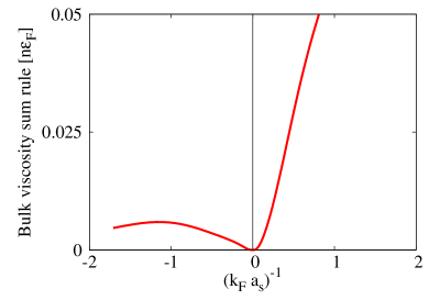
Figure 1: (Color online) The value of the bulk viscosity sum rule given by the right-hand side of Eq. (69) at $T=0$ in units of $n\epsilon_{F}$ through the BCS-BEC crossover.

We see from Eq. (69) that the bulk viscosity sum rule vanishes at unitarity:

$$\frac{1}{\pi}\int^{\infty}_{0}d\omega\;\zeta(\omega)=0\ \ \ \ (|a|=\infty).$$ (75)

We are using here the fact that $(\partial C/\partial a^{-1})_{s}$ is finite (i.e., non-infinite) at $x=1/(k_{F}a)=0$ at all temperatures. One can also see this using elementary arguments that do not involve the contact. From “universal thermodynamics” Ho04 , the only energy scales at unitarity are $\epsilon_{F}$ and the temperature, and we can directly show that $P-\varepsilon/9-\rho c_{s}^{2}/2=0$ (see Appendix E).

The vanishing sum rule, Eq. (75), together with the positivity condition $\zeta(\omega)\geq 0$ derived in Section IV, implies

$$\zeta(\omega)=0\ \ \ \forall\omega\ \ \ (|a|=\infty).$$ (76)

That the static bulk viscosity $\zeta(0)$ vanishes is a well-known consequence Son07 of scale or conformal invariance at unitarity Castin04 . Our result generalizes this to arbitrary frequencies. As discussed below in Section IX, our result actually has important implications for measuring the frequency dependent shear viscosity of a unitary Fermi gas using a density probe such as two-photon Bragg scattering.

Another general consequence of $\zeta(\omega)\geq 0$ is that its sum rule must be positive for all $x=1/(k_{F}a)$ and $T$. Equation (69) then implies that

$$\left(\frac{\partial C}{\partial a^{-1}}\right)_{{s}}\geq 0\;\;\;\;\forall a,$$ (77)

so that the contact must be a monotonically increasing function of $1/(k_{F}a)$ through the BCS-BEC crossover at fixed entropy per particle. We can understand this inequality intuitively as follows: the contact $C$, which is related to the probability of finding two particles of opposite spin close to each other, can only increase with increasing attraction $a^{-1}$.

In Fig. 1 we show the bulk viscosity sum rule in Eq. (69) at $T=0$ calculated using QMC data Astrakharchik04 for the energy density $\varepsilon$. The contact $C$ is obtained from $\varepsilon$ using Tan’s “adiabatic relation” Tan08

$$\left(\partial\varepsilon/\partial a^{-1}\right)_{s}=-C/(4\pi m),$$ (78)

where the derivative is taken at fixed entropy per particle $s\equiv S/N$. We fitted the QMC data and took numerical derivatives with respect to $a^{-1}$. Since the $\zeta$ sum rule involves the second derivative of QMC data for the energy density, the results may not be very accurate far from unitarity in either direction.

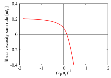
Figure 2: (Color online) The value of the finite shear viscosity sum rule, with the contribution from the high-frequency tail in Eq. (72) subtracted out, given by the right-hand side of Eq. (71) at $T=0$ in units of $n\epsilon_{F}$ through the BCS-BEC crossover.

Both the vanishing of the $\zeta$ sum rule at $x=1/(k_{F}a)=0$ and its positivity away from unitarity are apparent in Fig. 1. This is due to the $1/a^{2}$ dependence of the sum rule in the vicinity of unitarity. We emphasize the nontriviality of the result given by Eq. (69) in the unitarity region. In the form first derived in Eq. (68), the right hand side is $(P-\varepsilon/9-\rho c_{s}^{2}/2)$. Each term in this expression has both constant and order $x$ contributions, which must all cancel to give a final result which goes like $x^{2}$ at small $x$. In the BCS limit, the $\zeta$ sum rule vanishes as $2n\epsilon_{F}/(27\pi|x|$) since $C\to 4\pi^{2}n^{2}a^{2}_{s}$ Tan08 . In the BEC limit, the energy density is dominated by the negative molecular binding energy, $\varepsilon\approx nE_{b}/2$, with $E_{b}=-1/(ma^{2})$. Thus, $C\to 4\pi n/a$ and the sum rule grows as $n|E_{b}|/18$.

Next, in Fig. 2, we plot the shear viscosity sum rule given by Eq. (71) at $T=0$ again using the QMC data of Ref. Astrakharchik04 . Because of the $1/\sqrt{\omega}$ subtraction extending all the way down to $\omega=0$, the $\eta$ sum rule in Eq. (71) is not constrained to be positive. Using the above analytic result for the contact in the BCS limit, one finds that the $\eta$ sum rule asymptotes to $0.2n\epsilon_{F}$ in the BCS limit. At unitarity, $|a|=\infty$ and the $\eta$ sum rule is $\varepsilon/3\simeq 0.4\times(3n\epsilon_{F}/5)\times(1/3)=0.08n\epsilon_{F}$. On the BEC side of the resonance the sum rule changes sign, tending to $(17/30)nE_{b}$ in the BEC limit.

IX Dynamic Structure Factor

We now discuss the connection between viscosity and the density-density correlator or dynamic structure factor. This analysis leads to two interesting results for the two-component Fermi gas. First, we predict that a density probe such as two-photon Bragg spectroscopy Iacuppo can in principle be used to measure the frequency dependent $\eta(\omega)$ at unitarity:

$$\eta(\omega)=\lim_{q\to 0}\frac{3\omega^{3}}{4q^{4}}\;\mathrm{Im}\chi_{\rho\rho}({\bf q},\omega)\ \ \ \ \ (|a|=\infty).$$ (79)

Second, we derive the high-frequency tail Son10

$$\lim_{\omega\to\infty}\lim_{q\to 0}S({\bf q},\omega)=\frac{2q^{4}C}{15\pi^{2}m^{1/2}}\frac{1}{\omega^{7/2}},$$ (80)

a result that is valid for all $1/(k_{F}a)$ and all temperatures. As discussed below, such non-analytic tails are also known in other strongly interacting quantum fluids like ⁴He.

We start with the operator form of the continuity equation

$$i[\hat{\rho},\hat{H}]=m\partial_{\alpha}\hat{j}_{\alpha},$$ (81)

where $\hat{\rho}=m\hat{n}$ is the mass density operator, and take its matrix elements between exact many-body eigenstates. Using the spectral representation, Eq. (12), we relate the density correlator $\chi_{\rho\rho}$ to the the longitudinal current correlator [see Eq. (92)]. The latter is related to the viscosity as shown in Eq. (21), namely $\zeta(\omega)+4\eta(\omega)/3=\lim_{q\to 0}{m^{2}\omega}\mathrm{Im}\chi_{L}({\bf q},\omega)/{q^{2}}$. We thus obtain

$$\zeta(\omega)+{4\eta(\omega)}/{3}=\lim_{q\to 0}{\omega^{3}}\mathrm{Im}\chi_{\rho\rho}({\bf q},\omega)/{q^{4}}.$$ (82)

We discuss two situations where the contribution of $\zeta(\omega)$ vanishes and we can obtain interesting results connecting $\eta(\omega)$ and density correlations.

First, we focus on the unitary Fermi gas where $\zeta(\omega)$ vanishes at all $\omega$ (as shown in Section VIII) and Eq. (82) simplifies to Eq. (79). Thus, the frequency-dependent shear viscosity $\eta(\omega)$ in a unitary Fermi gas can in principle be measured using an experiment like Bragg scattering, which directly probes $\mathrm{Im}\chi_{\rho\rho}$.

Second, let us look at the high-frequency regime $\epsilon_{F}\ll\omega\lesssim 1/(mr_{0}^{2})$. The $\zeta$ sum rule in Eq. (68) is convergent in the $r_{0}\to 0$ limit, and thus $\zeta(\omega)$ must decay faster than $1/\omega$, while $\eta(\omega)\sim 1/\sqrt{\omega}$ (see Section VII). Thus, as $\omega\to\infty$, the bulk viscosity $\zeta(\omega)$ is much smaller than the shear viscosity $\eta(\omega)$ for all $1/(k_{F}a)$ and all $T/\epsilon_{F}$. Using Eq. (82) we thus find

$$\eta(\omega\to\infty) \simeq \lim_{\omega\to\infty}\lim_{q\to 0}\frac{3\omega^{3}}{4q^{4}}\mathrm{Im}\chi_{\rho\rho}({\bf q},\omega)$$ (83)

$$= \lim_{\omega\to\infty}\lim_{q\to 0}\frac{3\pi\omega^{3}}{4q^{4}}S({\bf q},\omega),$$

The dynamic structure factor $S({\bf q},\omega)$ is related to $\mathrm{Im}\chi_{\rho\rho}$ via the fluctuation-dissipation theorem

$$S({\bf q},\omega)=\frac{\mathrm{Im}\chi_{\rho\rho}({\bf q},\omega)}{\pi[1-\exp(-\beta\omega)]}.$$ (84)

Our final result, given by Eq. (80), for the high-frequency tail of $S({\bf q},\omega)$ is obtained by using the high-frequency tail, Eq. (72), of $\eta(\omega)$ in Eq. (83).

The high-frequency $\omega^{-7/2}$ tail of the dynamic structure factor result is a universal feature of short-range two-body interactions. Remarkably, such a tail was first noticed in deep inelastic neutron scattering studies of superfluid ⁴He Wong77 and was subsequently understood in terms of hard-sphere gases Kirkpatrick84 . The high-frequency neutron scattering experiments probe the short distance properties of the two-body pair distribution function. [In dilute Fermi gases, this is directly related to the contact $C$; see Eq. (59)]. It may seem surprising that such anomalous high-frequency tails arise even in dense systems like ⁴He. Recall that this behavior should be visible in a frequency range $n^{2/3}/m<\omega<1/mr^{2}_{0}$ in which the interaction “looks” short-range. Even in ⁴He, where $nr^{3}_{0}\lesssim 1$, such a frequency range can be found using deep inelastic neutron scattering, although the range is obviously much smaller than in dilute gases with $nr^{3}_{0}\ll 1$.

X Comparison with sum rules for Relativistic Field Theories

There has been a considerable effort in the high-energy literature to understand the properties of viscosity spectral functions and their sum rules; see, e.g., Refs. Teaney06 ; Romatschke09 ; Moore08 ). In addition to understanding the transport coefficients within the AdS/CFT framework, this work seems to be motivated in part by an interest in reliably extracting transport coefficients of the quark-gluon plasma from lattice QCD calculations of Euclidean correlation functions. We briefly discuss here some similarities and differences between the results for relativistic quantum field theories and those derived in this paper for non-relativistic Fermi gases: Eqs. (69) and (71).

There exist a number of Boltzmann calculations of the viscosity spectral functions in weak coupling QCD Teaney06 ; Schafer09 . For the shear viscosity, the authors of Ref. Schafer09 find the shear viscosity sum rule

$$\frac{1}{\pi}\int^{\omega_{c}}_{0}d\omega\eta(\omega)=\frac{\varepsilon+P}{5},$$ (85)

where $g^{4}T\ll\omega_{c}\ll g^{2}T$ is a cutoff that removes a diverging contribution from a high-frequency tail. For the ${\cal{N}}=4$ supersymmetric Yang-Mills theory (SYM), Romatschke and Son Romatschke09 derived the following shear viscosity sum rule:

$$\frac{1}{\pi}\int^{\infty}_{0}d\omega[\eta(\omega)-\eta_{T=0}(\omega)]=\frac{\varepsilon}{5}.$$ (86)

Here, a diverging vacuum contribution from a $T$-independent high-frequency tail has been subtracted out. We note that our $\eta$ sum rule in Eq. (71), though similar in structure, has one key difference. The high-frequency tail for the Fermi gas is in general $T$-dependent, because its coefficient is set by the contact $C=k_{F}^{4}{\cal C}[1/(k_{F}a),T/\epsilon_{F}]$.

A non-perturbative calculation of the bulk viscosity sum rule in ${\cal{N}}=4$ supersymmteric Yang-Mills theory and pure Yang-Mills theory (QCD with no quarks) has been given recently by Romatschke and Son Romatschke09 :

$$\frac{1}{\pi}\int^{\infty}_{0}d\omega[\zeta(\omega)-\zeta_{T=0}(\omega)]=$$ (87)

$$(3\varepsilon+P)(1-3c^{2})-4(\varepsilon-3P),$$

where $c\equiv\sqrt{\partial P/\partial\varepsilon}$ is the sound speed in relativistic hydrodynamics (with the speed of light equal to unity) LLFM . There are some differences and one very interesting similarity with our $\zeta$ sum rule in Eq. (69). In contrast to the Fermi gas spectral function $\zeta(\omega)$, there is a need to subtract out a divergent tail in Eq. 87 and this tail appears to be $T$-independent. The interesting similarity is that in the “conformal limit” $P=\varepsilon/3$, the right hand side of Eq. (87) vanishes, analogous to the unitary Fermi gas.

XI Conclusions

In this paper we have derived various exact, non-perturbative results for the shear and bulk viscosities of non-relativistic quantum fluids, focusing on the strongly interacting Fermi gas. Our main results were already summarized in the Introduction. To conclude, we discuss some open questions and how our results relate to them.

Most calculations Bruun05 ; Schafer07 of the viscosity in strongly interacting Fermi gases have so far been restricted to solving Boltzmann equations or using diagrammatic perturbation theory, in essence making a quasiparticle approximation. Such results are valid in the high and low temperature regimes, but not in the most interesting regime near and above $T_{c}$ where a quasiparticle approximation is questionable and the shear viscosity is known to be the smallest. It was recognized some time back Randeria-reviews that there is a breakdown of Fermi liquid theory in the normal (i.e., non-superfluid) state of the strongly interacting regime of the BCS-BEC crossover. It was shown that precursor pairing correlations lead to a pseudogap Randeria-reviews , which is a strong suppression of low-energy spectral weight in various response functions. It is likely that no sharp quasiparticle excitations exist in this regime near unitarity and just above $T_{c}$, but controlled calculations of dynamic quantities are very difficult.

Quantum Monte Carlo methods have played an important role in determining the equilibrium thermodynamic properties of the unitary Fermi gas. However, results for transport coefficients are much less common, since they require analytic continuation of imaginary time (Euclidean) data to the real axis Aarts02 . The sum rules we derive could serve as useful constraints on similar calculations for strongly interacting Fermi gases.

From an experimental point of view, the (static) shear viscosity for strongly interacting Fermi gases has been estimated from studies of the damping of collective oscillations Turlapov08 . We have shown above that, at unitarity, the full frequency dependence of the shear viscosity spectral function $\eta(\omega)$ can be obtained from two-photon Bragg spectroscopy. While it would be a challenging experiment (the density response being very small for small-$q$), this would give extremely important insights into the strongly interacting Fermi gas, analogous to optical conductivity measurements of solids.

Finally, we return to the conjectured bound Son-review on the shear viscosity, Eq. (1). Proving or disproving the existence of a bound bound for non-relativistic quantum fluids like the strongly interacting Fermi gas remains a challenging open problem. We hope that the spectral functions and sum rules derived here constitute a step in this direction, just as they have for other well known inequalities in quantum many-body physics.

Appendix A Modified stress correlator

In the main paper we discussed current correlator and stress correlator representations of the bulk and shear viscosities. Here, we describe a third correlation function using an explicitly defined operator $\widehat{\Pi}^{0}_{\alpha\beta}$ which has been used to calculate the static shear viscosity $\eta=\mathrm{Re}\;\eta(\omega=0)$. We note that $\widehat{\Pi}^{0}$, which does not include the diagonal terms of the full stress tensor, cannot be used to calculate the bulk viscosity.

Let us define

$$\hat{\Pi}^{0}_{\alpha\beta}({\bf r})=\frac{1}{2m}\sum_{i=1}^{N}\left\{\hat{{\bf p}}^{i}_{\alpha}\hat{{\bf p}}^{i}_{\beta},\delta({\bf r}-\hat{{\bf r}}_{i})\right\}$$ (88)

where $\hat{{\bf p}}^{i}_{\alpha}$ is the $\alpha$-component of the momentum operator for the $i$-th particle. We emphasize that this is only one piece – the kinetic part – of the full stress tensor operator, and omits other terms, such as the pressure. It is independent of the interaction potential unlike the full stress tensor. However, since the expectation value of the “off-diagonal” part of $\widehat{\Pi}^{0}$ is identical to the hydrodynamic stress tensor in Eq. (6), we expect that we can use $\widehat{\Pi}^{0}$ to compute the shear viscosity, at least in the low frequency limit.

We define the correlator $\chi^{xy,xy}_{\Pi^{0}}$ by choosing $\hat{A}=\hat{\Pi}^{0}_{\alpha\beta}({\bf q})$ and $\hat{B}=\hat{\Pi}^{0}_{\mu\nu}(-{\bf q})$ in Eq. (12), where

$$\hat{\Pi}^{0}_{\alpha\beta}({{\bf q}})=\frac{1}{4m}\sum_{{\bf k}\sigma}\hat{c}^{\dagger}_{{\bf k}\sigma}\hat{c}_{{\bf k}+{\bf q}\sigma}(2k_{\alpha}+q_{\alpha})(2k_{\beta}+q_{\beta}).$$ (89)

We can write the analog of Eq. (26) as

$$\eta_{0}(\omega)=\lim_{q\to 0}\mathrm{Im}\chi^{xy,xy}_{\Pi^{0}}/\omega.$$ (90)

This is the form used by several authors Bruun05 ; Peshier05 as a starting point for diagrammatic approximations.

The sum rule for the modified stress correlator, Eq. (89), simply follows from the Kramers-Kronig relation:

$$\frac{1}{\pi}\int^{\infty}_{0}d\omega\lim_{q\to 0}\frac{\mathrm{Im}\chi^{xy,xy}_{\Pi^{0}}({\bf q},\omega)}{\omega}=$$ (91)

$$\lim_{\omega\to 0}\lim_{q\to 0}\frac{1}{2}\mathrm{Re}\chi^{xy,xy}_{\Pi^{0}}({\bf q},\omega).$$

Ironically, it is seems harder to explicitly evaluate the right hand side here than it is to calculate the exact sum rule in Eq. (55), despite the simple operator $\widehat{\Pi}^{0}$ involved. The point is that $\hat{\Pi}^{0}$ does not satisfy the Euler equation, Eq. (22), and hence we cannot relate it to the current. Thus, in contrast to the sum rules given by Eqs. (47) and (48) which involve the first frequency moment of the current correlator, we must deal directly with an inverse frequency moment in Eq. (91). Such an inverse moment is a generalized “static susceptibility”, about which we do not seem to know much, at least in this case. Unlike positive moment sum rules, it cannot be written in terms of commutators.

Appendix B Hydrodynamics

In this Appendix, we review well-known hydrodynamic results for the current correlation functions Kadanoff63 ; Hohenberg65 . To keep the discussion as general as possible, we will use the full two-fluid hydrodynamic correlation functions that result from solving the linearized equations of two-fluid hydrodynamics LLFM ; ZNGbook . As written below, these correlation functions describe any superfluid with a two-component order parameter, including dilute two-component Fermi gases (see Ref. Taylor09 and references therein), and reduce to standard hydrodynamic expressions in the normal phase above $T_{c}$. We start by writing down a relation between the longitudinal current correlation function $\chi_{L}({\bf q},\omega)$ and the (mass) density response function $\chi_{\rho\rho}({\bf q},\omega)$. (Recall that our current correlation function is the number current correlation function and not the mass current correlation function generally used in the older literature Kadanoff63 ; Hohenberg65 . We will find it convenient in the analysis below to use the correlation function $\chi_{\rho\rho}$ for the mass density $\rho=mn$, however.) Analogous to the result given by Eq. (LABEL:Correlationrelation), the continuity equation $\partial_{t}n+{\bm{\nabla}}\cdot\bm{j}=0$ can be used to find

$$\omega^{2}\chi_{\rho\rho}({\bf q},\omega) = (mq)^{2}\chi_{L}({\bf q},\omega)-{\bf q}\cdot\langle[\hat{\bm{j}}_{{\bf q}},\hat{\rho}_{-{\bf q}}]\rangle$$ (92)

$$= (mq)^{2}\chi_{L}({\bf q},\omega)-\rho q^{2}.$$

We can now use the hydrodynamic expression for $\chi_{\rho\rho}({\bf q},\omega)$ to obtain an explicit hydrodynamic expression for $\chi_{L}({\bf q},\omega)$. In the hydrodynamic regime, the density response function is (see, e.g., Eq. (4.32) in Ref. Hohenberg65 ):

$$\frac{\chi_{\rho\rho}({\bf q},\omega)}{\rho q^{2}}=$$ (93)

$$\!\!\!\!\!\!\!\!\frac{-\omega^{2}+q^{2}\frac{\rho_{s}Ts^{2}}{\rho_{n}c_{v}}-iq^{2}\omega\Gamma}{(\omega^{2}-u^{2}_{1}q^{2}+iD_{1}q^{2}\omega)(\omega^{2}-u^{2}_{2}q^{2}+iD_{2}q^{2}\omega)}.$$

Here, $u_{1}$ and $u_{2}$ are the speeds of first and second sound, respectively. They can be shown to satisfy the following identity (see, e.g., Eq. (14.39) in Ref. ZNGbook ):

$$u^{2}_{1}+u^{2}_{2}=\frac{\rho_{s}Ts^{2}}{\rho_{n}c_{v}}+c^{2}_{s}\ \ \ {\rm with}\ \ \ c^{2}_{s}=\left({\partial P}/{\partial\rho}\right)_{s}.$$ (94)

Recall that $s\equiv S/N$ is the entropy per particle. $c_{v}\equiv T(\partial s/\partial T)_{\rho}$ is the specific heat per unit mass at constant volume. $\rho_{s}$ and $\rho_{n}$ are the superfluid and normal fluid densities. The damping coefficients $\Gamma$, $D_{1}$, and $D_{2}$ obey the following identities:

$$\Gamma\equiv\frac{\kappa}{\rho c_{v}}+\frac{\rho_{s}}{\rho_{n}}\left(\frac{4\eta/3+\zeta_{2}}{\rho}-2\zeta_{1}+\rho\zeta_{3}\right)$$ (95)

and

$$D_{1}+D_{2}=\Gamma+\frac{1}{\rho}\left(4\eta/3+\zeta_{2}\right).$$ (96)

Here, $\kappa$ is the thermal conductivity and $\zeta_{1}$, $\zeta_{2}$, and $\zeta_{3}$ are the bulk viscosities associated with the different types of motion that can arise in the superfluid phase LLFM . Above $T_{c}$, $\zeta_{2}$ reduces to the usual bulk viscosity $\zeta$ and the remaining bulk viscosities do not contribute.

After some straightforward but lengthy algebra, one can show from Eqs. (92) and (93) that

$$\lim_{\omega\to 0}\lim_{q\to 0}\frac{m^{2}\omega^{2}}{2q^{2}}\mathrm{Re}\chi_{L}({\bf q},\omega)\!=\!-\frac{\rho}{2}\left[u^{2}_{1}+u^{2}_{2}-\frac{\rho_{s}Ts^{2}}{\rho_{n}c_{v}}\right].$$

Using Eq. (94) in this expression gives the result in Eq. (LABEL:difference2).

The transverse current correlation function is given by (see Eq. (4.49) in Ref. Hohenberg65 )

$$m^{2}\chi_{T}({\bf q},\omega)=\frac{\eta q^{2}}{\eta q^{2}/\rho_{n}-i\omega}.$$ (98)

From Eq. (98), we see that the real part of the transverse current correlation function is proportional to $q^{4}$, leading to the result in Eq. (LABEL:difference2).

Appendix C Contact

This Appendix consists of two parts. In the first part, we briefly recall, for completeness, some basic properties of Tan’s contact; more details may be found in the original references Tan08 ; Braaten08 . In the second part, we use the same techniques, within a real-space formulation Zhang08 , to derive Eqs. (64) and (65) for $\overline{V}^{\prime}$ and $\overline{V}^{\prime\prime}$.

The contact $C$ can be defined by the large-$k$ tail of the momentum distribution function $\lim_{k\to\infty}n_{{\bf k}}={C}/{k^{4}}$. This leads to a kinetic energy density $\langle\hat{K}\rangle=2\int d^{3}{\bf k}\;(k^{2}/2m)\;n_{{\bf k}}$ with a linearly divergent piece that goes like $C\Lambda/(2\pi^{2}m)$, where $\Lambda\equiv 1/r_{0}$ is the ultraviolet cutoff. The potential energy density is given by Braaten08

$$\langle\hat{V}\rangle=\frac{C}{4\pi ma}-\frac{\Lambda C}{2\pi^{2}m},$$ (99)

so that the total energy density $\varepsilon=\langle\hat{K}\rangle+\langle\hat{V}\rangle$ is finite in the $\Lambda=1/r_{0}\to\infty$ limit. We will freely use these results, together with those obtained from the short-distance properties of two-body density matrix, to evaluate the quantities of interest for our sum rules.

At short distances, $r_{0}\lesssim r\ll k^{-1}_{F}$, the two-body density matrix for a two-component dilute Fermi gas has the structure Zhang08

$$\int\!\!d^{3}{\bf R}\Big{\langle}\hat{\psi}^{\dagger}_{\uparrow}({\bf R}\!+\!\frac{{\bf r}}{2})\hat{\psi}^{\dagger}_{\downarrow}({\bf R}\!-\!\frac{{\bf r}}{2})\hat{\psi}_{\downarrow}({\bf R}\!-\!\frac{{\bf r}}{2})\hat{\psi}_{\uparrow}({\bf R}\!+\!\frac{{\bf r}}{2})\Big{\rangle}$$

$$\equiv{\cal F}({\bf r})=\frac{C}{16\pi^{2}}\left(\frac{1}{r}-\frac{1}{a}\right)^{2}.$$ (100)

Let us use this to compute the interaction energy density

$$\langle\hat{V}\rangle=\frac{C}{4\pi}\int drV(r)\left(1-{r}/{a}\right)^{2}.$$ (101)

It is easy to see that for $r_{0}\to 0$, we may drop the $(r/a)^{2}$ term in the integrand as it gives a vanishingly small contribution. Using

$$X_{n}=\frac{C}{4\pi}\int drV(r)(r/a)^{n}\ \ \ \ (n=0,1)$$ (102)

we thus obtain

$$\langle\hat{V}\rangle=X_{0}-2X_{1}.$$ (103)

Similarly, Eqs. (60) and (61) may be written as

$$\overline{V}^{\prime}=-X_{0}+4X_{1}$$ (104)

and

$$\overline{V}^{\prime\prime}=2X_{0}-12X_{1}.$$ (105)

Next, we wish to determine the integrals $X_{0}$ and $X_{1}$ in the limit where the range of the potential vanishes: $r_{0}\to 0$. Comparing the results given by Eqs. (99) and (103) for $\langle\hat{V}\rangle$, it is evident that $X_{0}$ is linearly divergent in $\Lambda$ and $X_{1}$ is finite as $\Lambda=1/r_{0}\to\infty$. But there is no way to determine the finite part of $X_{0}$ from this comparison alone. We need one additional piece of information to determine $X_{0}$ and $X_{1}$. We get this from the relation

$$P={2}\varepsilon/3+\langle\hat{V}\rangle/{3}+\overline{V}^{\prime}/{3}.$$ (106)

for the pressure $P$ which is derived in Appendix D. Using Eqs. (103) and (104), we see that the divergent terms ($X_{0}$) cancel and the pressure

$$P={2}\varepsilon/{3}+{2}X_{1}/3$$ (107)

is finite as $r_{0}\to 0$. Comparing this with Tan08 $P=2\varepsilon/3+{C}/(12\pi ma)$ we obtain

$$X_{1}={C}/(8\pi ma).$$ (108)

Substituting this into Eq. (103) for $\langle\hat{V}\rangle$, and comparing with Eq. (99), we find

$$X_{0}=-C\Lambda/(2\pi^{2}m)-{C}/(2\pi ma).$$ (109)

Using these results for $X_{0}$ and $X_{1}$ in Eqs. (104) and (105) we obtain Eqs. (64) and (65) for $\overline{V}^{\prime}$ and $\overline{V}^{\prime\prime}$, respectively.

Appendix D Pressure

In the main text of this paper, we have suppressed factors of the volume $\Omega$ at all places by setting it equal to unity. In this Appendix, we re-introduce factors of $\Omega$ in order to use the thermodynamic relation $P=-(\partial F/\partial\Omega)_{T,N}$ to derive a microscopic expression for the pressure. To evaluate this, we use the Feynman-Hellmann formula $(\partial F/\partial\lambda)_{T,N}=\langle\partial\hat{H}/\partial\lambda\rangle$ treating the volume $\Omega$ as a parameter $\lambda$ in the Hamiltonian

$$\hat{H}=\sum_{{\bf k}\sigma}\varepsilon_{{\bf k}}\hat{c}^{\dagger}_{{\bf k}\sigma}\hat{c}_{{\bf k}\sigma}\!+\!\frac{1}{\Omega}\!\sum_{{\bf k}{\bf k}^{\prime}{\bf p}}V(p)\hat{c}^{\dagger}_{{\bf k}+{\bf p}\uparrow}\hat{c}^{\dagger}_{{\bf k}^{\prime}-{\bf p}\downarrow}\hat{c}_{{\bf k}^{\prime}\downarrow}\hat{c}_{{\bf k}\uparrow}.$$ (110)

The volume enters in two ways: (i) explicitly, though the $\Omega^{-1}$ factor in front of the interaction term, and (ii) implicitly, through the discrete wavevectors ${\bf k}=\left(2\pi/\Omega^{1/3}\right)(n_{x},n_{y},n_{z})$. One can replace the momentum sums by sums over the discrete indices $n_{\alpha}=0,1,...$, and the operators only depend on these indices. Thus, in addition to the explicit $\Omega^{-1}$ factor, the kinetic energy $\varepsilon_{{\bf k}}={\bf k}^{2}/2m$ and the two-body potential $V(p)$ also depend on the volume $\Omega$.

Using $3\Omega\left[\partial F({\bf k})/\partial\Omega\right]=-k_{\alpha}\left[\partial F({\bf k})/\partial k_{\alpha}\right]$ (with the summation convention) and the definition of $\overline{V}^{\prime}$ given in Eq. (54), we find the result

$$P=\frac{2}{3}\varepsilon+\frac{1}{3}\langle\hat{V}\rangle+\frac{1}{3}\overline{V}^{\prime}.$$ (111)

Appendix E Thermodynamics of the BCS-BEC Crossover

In this Appendix, we simplify the form of the bulk viscosity sum rule in Eq. (68) and derive the result given by Eq. (69) using thermodynamic scaling arguments Ho04 and the Tan relations Tan08 . We begin by writing the energy density of a two-component Fermi gas in the scaling form

$$\varepsilon=n\epsilon_{F}{\cal{E}}(x,s),$$ (112)

which is valid across the entire BCS-BEC crossover. Here, ${\cal{E}}$ is a dimensionless function of the interaction parameter $x=1/(k_{F}a)$ and the entropy per particle $s\equiv S/N$. We find it convenient to use $s$, rather then more familiar variable $T/\epsilon_{F}$, because we will need to evaluate adiabatic derivatives below. The density dependence of the Fermi energy and Fermi wavevector are given by $\epsilon_{F}=(3\pi^{2}n)^{2/3}/2m$ and $k_{F}=(3\pi^{2}n)^{1/3}$ respectively, and $a$ is the $s$-wave scattering length.

We first calculate the adiabatic sound speed which enters the right hand side of the $\zeta$ sum rule in Eq. (68). Using the definition $c_{s}^{2}=(\partial P/\partial\rho)_{s}$, where $\rho=mn$, together with Tan’s pressure relation, Eq. (63), we find

$$\frac{\rho c_{s}^{2}}{2}=\frac{n}{2}\left[\frac{2}{3}\left(\frac{\partial\varepsilon}{\partial n}\right)_{s}+\frac{1}{12\pi ma}\left(\frac{\partial C}{\partial n}\right)_{s}\right].$$ (113)

The derivatives at constant $s$ are evaluated as follows. The first term is $({\partial\varepsilon}/{\partial n})_{s}=(5\varepsilon/3n)-(\epsilon_{F}x/3)({\partial{\cal{E}}}/{\partial x})_{s}$. We compute $({\partial{\cal{E}}}/{\partial x})_{s}$ using Tan’s adiabatic relation, Eq. (78), and obtain $n({\partial\varepsilon}/{\partial n})_{s}=5\varepsilon/3-C/(12\pi ma)$. To calculate the second term in Eq. (113), we rewrite the contact in the scaling form

$$C=k^{4}_{F}\widetilde{C}(x,s)$$ (114)

where $\widetilde{C}$ is a dimensionless function on its arguments. After some simple algebra, we find $n({\partial C}/{\partial n})_{s}=4C/3-(3a)^{-1}({\partial C}/{\partial a^{-1}})_{s}$. Adding up all of the contributions to the bulk viscosity sum rule, we find

$$\frac{5\varepsilon}{9}+\frac{C}{12\pi ma}-\frac{\rho c_{s}^{2}}{2}=\frac{1}{72\pi ma^{2}}\left(\frac{\partial C}{\partial a^{-1}}\right)_{s}.$$ (115)

That the $\zeta$ sum rule vanishes at unitarity can also be seen directly from thermodynamic scaling arguments, without introducing the contact. Using Eq. (112), we see that $P=-(\partial(\varepsilon\Omega)/\partial\Omega)_{S,N}=2\varepsilon/3$ at unitarity [as anticipated by Eq. (63)] Thomas05 . Using this, we also find that the adiabatic sound speed at all temperatures is given by $c^{2}_{s}=(1/m)\left(\partial P/\partial n\right)_{s}=5P/3\rho$. Combining these results, one immediately obtains the result in Eq. (75) that the bulk viscosity sum rule vanishes there.

References

- (1) D. T. Son and A. O. Starinets, Ann. Rev. Nucl. Part. Sci. 57, 95 (2007) [arXiv:0704.0240].
- (2) For a recent review, see T. Schäfer and D. Teaney, Rep. Prog. Phys. 72, 126001 (2009).
- (3) P. K. Kovtun, D. T. Son, and A. O. Starinets, Phys. Rev. Lett. 94, 111601 (2005).
- (4) G. Policastro, D. T. Son, and A. O. Starinets, Phys. Rev. Lett. 87, 081601 (2001).
- (5) T. D. Cohen, Phys. Rev. Lett. 99, 021602 (2007); D. T. Son, Phys. Rev. Lett. 100, 029101 (2008).
- (6) M. Brigante, H. Liu, R. C. Myers, S. Shenker, and S. Yaida, Phys. Rev. Lett. 100, 191601 (2008).
- (7) Y. Kats and P. Petrov, JHEP01(2009)044.
- (8) A. Buchel, R. C. Myers, and A. Sinha, JHEP03(2009)084.
- (9) K. H. Ackermann et al. (STAR Collaboration), Phys. Rev. Lett. 86, 402 (2001).
- (10) D. Teaney, J. Lauret, and E. V. Shuryak, Phys. Rev. Lett. 86, 4783 (2001).
- (11) A. Turlapov, J. Kinast, B. Clancy, L. Luo, J. Joseph, and J. E. Thomas, Journ. Low Temp. Phys. 150, 567 (2008); J. E. Thomas, Nucl. Phys. A 830, 665c (2009).
- (12) B. A. Gelman, E. V. Shuryak, and I. Zahed, Phys. Rev. A 72, 043601 (2005).
- (13) S. Giorgini, L. P. Pitaevskii, and S. Stringari, Rev. Mod. Phys. 80, 1215 (2008).
- (14) S. Tan, Ann. Phys. 323, 2952 (2008); 323, 2971 (2008); 323, 2987 (2008).
- (15) D. T. Son, Phys. Rev. Lett. 98, 020604 (2007).
- (16) Dam Son has kindly informed us of his recent work where the same tail of the dynamic structure factor is derived using operator product expansions; D. T. Son and E. G. Thompson, arXiv:1002.0922.
- (17) L. D. Landau and E. M. Lifshitz, Fluid Mechanics (Elsevier, Oxford, 2004).
- (18) E. M. Lifshitz and L. P. Pitaevskii, Statistical Physics, Part 2 (Butterworth-Heinemann, Oxford, 2002).
- (19) For complicated expressions for the operator, which are hard to use, see, e.g., Eq. (4.6) of D. Forster, Hydrodynamics, Fluctuations, Broken Symmetry, and Correlation Functions (Perseus Books, Cambridge Massachusetts, 1990). A different, presumably equivalent, expression may be found in Eq. (B7) of Y. Nishida and D. T. Son, Phys. Rev. D 76, 086004 (2007). See, also, H. Mori, Phys. Rev. 111, 694 (1958) and M. J. Godfrey, Phys. Rev. B 37, 10176 (1988).
- (20) L. P. Kadanoff and P. C. Martin, Ann. Phys. 24, 419 (1963).
- (21) D. Pines and P. Nozières, The theory of quantum liquids, vol. I (Benjamin, New York, 1966).
- (22) G. Baym in Mathematical methods in solid state and superfluid theory, edited by R. C. Clark and G. H. Derrick (Oliver and Boyd, Edinburgh, 1969).
- (23) A Galilean shift such as that used to arrive at Eq. (8) is strictly only valid for a uniform velocity field . In this case, Eq. (8) gives the Hamiltonian in the rest frame of the “walls” bounding the system in accordance with the principle of Galilean relativity Baymbook . However, the fact that the velocity field is (necessarily) nonuniform means that translational symmetry is broken and there is no suitable reference frame in which the system can be in equilibrium. Nonetheless, in the long wavelength limit required to define the viscosity coefficients, Eq. (8) reduces to the Hamiltonian in the rest frame of the walls, meaning that it is suitable for defining equilibrium thermodynamic averages.
- (24) Consider, e.g., the induced current in the direction, and set . The transverse correlator is obtained by first taking the , followed by limit. Interchanging the order, one finds the longitudinal result.
- (25) G. M. Bruun and H. Smith, Phys. Rev. A 75, 043612 (2007).
- (26) A. Peshier and W. Cassing, Phys. Rev. Lett. 94, 172301 (2005).
- (27) See Chapters 4 and 6 of P. Nozières and D. Pines, The theory of quantum liquids, vol. II (Addison-Wesley, Redwood City, 1990).
- (28) See Section V of D. J. Scalapino, S. R. White and S. C. Zhang, Phys. Rev. B 47, 7995 (1993).
- (29) A lattice potential or a random potential that destroys continuous translational invariance leads to even at ; see A. Paramekanti, N. Trivedi, and M. Randeria, Phys. Rev. B 57, 11639 (1998).
- (30) We argue that . Otherwise, would have potentially divergent contributions. As discussed above, is analogous to the resistivity and does not have a piece. This is very different from superconductors which have a term in their frequency-dependent conductivity.
- (31) Note that the shear viscosity of a charge-neutral superfluid goes like as . The number of phonon excitations becomes vanishingly small (), but they have a diverging mean-free path (). Precisely at , there are no phonon excitations and vanishes. See, e.g., I. M. Khalatnikov, An Introduction to the Theory of Superfluidity (W. A. Benjamin, New York, 1965); Ch. 20.
- (32) P. M. Chaikin and T. C. Lubensky, Principles of condensed matter physics, (Cambridge, N.Y., 1995), Ch. 7.6.
- (33) See Ch. 7 in S. Stringari and L. P. Pitaevskii, Bose-Einstein Condensation (Oxford University Press, Oxford, 2003).
- (34) In the limit, the second commutator in Eq. (LABEL:chiJasymptote) diverges, leading to the non-analyticity in Eq. (72).
- (35) F. Dalfovo and S. Stringari, Phys. Rev. B 46, 13991 (1992).
- (36) R. D. Puff, Phys. Rev. 137, A406 (1965); N. Mihara and R. D. Puff, Phys. Rev. 174, 221 (1968).
- (37) S. Zhang and A. J. Leggett, Phys. Rev. A 79, 023601 (2009).
- (38) E. Braaten and L. Platter, Phys. Rev. Lett. 100, 205301 (2008).
- (39) Recall that in Eq. (62) comes from an ultraviolet cutoff imposed on the two-body -matrix. In the center-of-mass frame of the two-body scattering problem, this is equivalent to imposing an energy cutoff with reduced mass ; hence the cutoff in Eq. (70).
- (40) Z. Yu and G. Baym, Phys. Rev. A 73, 063601 (2006); M. Punk and W. Zwerger, Phys. Rev. Lett. 99, 170404 (2007); S. Zhang and A. J. Leggett, Phys. Rev. A 77, 033614 (2008).
- (41) W. Schneider, V. B. Shenoy, and M. Randeria, arXiv:0903.3006; W. Schneider and M. Randeria, Phys. Rev. A 81, 021601(R) (2010).
- (42) P. Pieri, A. Perali and G. C. Strinati, Nature Phys. 5, 736 (2009).
- (43) T.-L. Ho, Phys. Rev. Lett. 92, 090402 (2004).
- (44) Y. Castin, Comptes Rendus Physique 5, 407 (2004); F. Werner and Y. Castin, Phys. Rev. A 74, 053604 (2006).
- (45) G. E. Astrakharchik, J. Boronat, J. Casulleras, and S. Giorgini, Phys. Rev. Lett. 93, 200404 (2004).
- (46) I. Carusotto, J. Phys. B: At. Mol. Opt. Phys. 39, S211 (2006).
- (47) V. K. Wong, Phys. Lett. A 61, 455 (1977). See also, A. Griffin, Excitations in a Bose-condensed liquid (Cambridge University Press, Cambridge, 1993), Ch. 8.1.
- (48) T. R. Kirkpatrick, Phys. Rev. B 30, 1266 (1984).
- (49) P. Romatschke and D. T. Son, Phys. Rev. D 80, 065021 (2009).
- (50) D. Teaney, Phys. Rev. D 74, 045025 (2006).
- (51) G. D. Moore and O. Saremi, JHEP09(2008)015.
- (52) T. Schäfer, Phys. Rev. A 76, 063618 (2007).
- (53) M. Randeria, in Proceedings of the International School of Physics “Enrico Fermi” Course CXXXVI on High Temperature Superconductors edited by G. Iadonisi, J. R. Schrieffer, and M. L. Chiafalo, (IOS Press, 1998), p. 53 [cond-mat/9710223]; M. Randeria, N. Trivedi, A. Moreo, and R. T. Scalettar, Phys. Rev. Lett. 69, 2001, (1992), and N. Trivedi and M. Randeria, Phys. Rev. Lett. 75, 312 (1995).
- (54) For a lattice QCD calculation of the shear viscosity, see e.g., G. Aarts and J. Martinez Resco, JHEP04(2002)053.
- (55) For relativistic systems without a conserved density, is the natural quantity to look at. For non-relativistic systems, a more natural quantity to look at would be , where is the normal fluid density defined in Sec. III.
- (56) P. C. Hohenberg and P. C. Martin, Ann. Phys. (N.Y.) 34, 291 (1965).
- (57) A. Griffin, T. Nikuni and E. Zaremba, Bose-condensed gases at finite temperatures, (Cambridge, N.Y., 2009).
- (58) E. Taylor, H. Hu, X.-J. Liu, L. P. Pitaevskii, A. Griffin, and S. Stringari, Phys. Rev. A 80, 053601 (2009).
- (59) J. E. Thomas, J. Kinast, and A. Turlapov, Phys. Rev. Lett. 95, 120402 (2005).