Self-Excitation and Feedback Cooling of an Isolated Proton

Abstract

The first one-proton self-excited oscillator (SEO) and one-proton feedback cooling are demonstrated. In a Penning trap with a large magnetic gradient, the SEO frequency is resolved to the high precision needed to detect a one-proton spin flip. This is after undamped magnetron motion is sideband-cooled to a 14 mK theoretical limit, and despite random frequency shifts (typically larger than those from a spin flip) that take place every time sideband cooling is applied. The observations open a possible path towards a million-fold improved comparison of the $\overline{\rm{p}}$ and p magnetic moments.

The demonstration of a one-electron self-excited oscillator (SEO) SelfExcitedOscillator and one-electron feedback cooling FeedbackCoolingPRL eventually led to greatly improved measurements of the electron magnetic moment and the fine structure constant HarvardMagneticMoment2008 . An electron spin flip caused the SEO oscillation frequency to shift observably because of a magnetic gradient added to the Penning trap that held the electron.

This Letter reports the first one-proton SEO and the first one-proton feedback cooling. The SEO frequency is resolved at the very precise level needed to observe a spin flip of a single $\overline{\rm{p}}$ or p – opening a possible way to compare the $\overline{\rm{p}}$ and p magnetic moments SelfExcitedOscillator ; QuintAntiprotonAspirations a million times more precisely than current comparisons. To compensate for the $\overline{\rm{p}}$ and p moments being 650 times smaller than that of an electron, these observations took place in a smaller trap with a much larger gradient than sufficed for observing spin flips of free HarvardMagneticMoment2008 and bound MainzSummary2006 electrons. Feedback cooling promises to narrow the spin resonance linewidth and increase the transition rate.

Effective sideband cooling DehmeltMagneticBottle ; Review is essential for these measurements, to center the p or $\overline{\rm{p}}$ so that electric and magnetic anharmonicities do not mask the tiny frequency shifts that would signal spin flips. Sideband cooling is widely utilized not only in precision measurements of trapped particles, but also for the manipulation of qubits Entanglement2008 , the most precise clocks CompareAlAndHgIonClocks2008 , the cooling of neutral atoms in lattices SidebandCoolingOfNeutralAtoms1998 , and the cooling of mechanical resonators SidebandCoolingMechanicalResonator . The one-proton SEO and feedback cooling make it possible to directly investigate the outcome of sideband cooling to the low-temperature, theoretical limit WinelandFrequencyDivision ; Review , for a particle that has no internal degrees of freedom available for cooling. The observed distribution of proton magnetron states is at the 14 mK theoretical limit. Previous such investigations with an electron VanDyckMagnetronCoolingLimit ; Review reached only an energy 400 times higher than the desired low temperature limit, and investigations with an ion probed temperatures orders of magnitude higher QuintDoublePenningTrap ; OneIonTemperature . A complication due to the strong magnetic gradient required is that an application of sideband cooling randomly shifts the SEO frequency by an amount larger than the shift from a spin flip on average.

A single proton is suspended in a vertical $B=5.68$ Tesla field at the center of a cylindrically symmetric trap (Fig. 1) – stacked rings with a 3 mm inner radius. The electrodes and surrounding vacuum container are cooled to 4.2 K by a thermal connection to liquid helium. Cryopumping of the closed system made the vacuum better than $5\times 10^{-17}$ Torr in a similar system PbarMass , so collisions are not important. Appropriate potentials applied to copper electrodes (with an evaporated gold layer) in an open-access geometry OpenTrap make a very good electrostatic quadrupole near the trap center, while also maintaining an open access to the trap interior from either end.

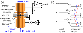
Figure 1: (a) Penning trap electrodes and radiofrequency schematic for feedback cooling and self-excitation of the proton axial motion. The feedback has gain $G$ and a phase shifted by $\phi$. (b) Energy levels and transitions (arrows) involved in axial sideband cooling of proton magnetron motion.

The proton’s circular cyclotron motion is perpendicular to B, with a frequency $\omega_{+}/(2\pi)=79.5$ MHz that is slightly modified by the electrostatic potential. The proton also oscillates parallel to B at $\omega_{z}/(2\pi)=\,553$ kHz. Because the potential is not a perfect quadrupole, this frequency depends slightly upon oscillation amplitude, $A$, with $\omega_{z}(A)\approx\omega_{z}$. The proton’s third motion is a circular magnetron motion, also perpendicular to B, at the much lower frequency, $\omega_{-}/(2\pi)=1.9$ kHz.

To couple the proton spin moment and the magnetron state that is the outcome of sideband cooling to the measurable $\omega_{z}(A)$, the trap’s central ring electrode is made of saturated iron (unlike the copper endcap and compensation electrodes above and below). The extremely large magnetic bottle gradient,

$$\Delta{\bf B}=\beta_{2}[(z^{2}-\rho^{2}/2){\bf\hat{z}}-z\rho\bm{\hat{\rho}}]$$ (1)

with $\beta_{2}=7.8\times 10^{4}$ T/m², is 51 and 8 times larger than what was used to measure free HarvardMagneticMoment2008 and bound QuintDoublePenningTrap ; MainzSummary2006 electron magnetic moments. The bottle reduces the field within the trap by $0.47$ T (8 %).

The axial frequency $\omega_{z}(A)$ depends primarily on the strength of the $z^{2}$ term in the electrostatic quadrupole. A magnetic moment $\mu\bf\hat{z}$ (from circular cyclotron or magnetron motions, or from spin) adds a term going as $\mu z^{2}$ to the trapping potential, shifting $\omega_{z}(A)$ by

$$\frac{\Delta\omega_{z}}{\omega_{z}}\approx\frac{\hbar\beta_{2}}{2m_{p}\omega_{-}|B|}\left(n+\frac{1}{2}+\frac{g_{p}m_{s}}{2}+\frac{\omega_{-}}{\omega_{+}}(\ell+\frac{1}{2})\right).$$ (2)

The magnetic moments from cyclotron and magnetron motion go as $n$ and $\ell$. The 553 kHz axial frequency shifts by $21$ mHz per cyclotron quantum ($200$ Hz per $\mu$m for our typical cyclotron radius), and by $0.5$ $\mu$Hz per magnetron quantum (40 mHz per $\mu m$ at our typical magnetron radius). A proton spin flip will cause a 60 mHz shift.

The frequency of the current induced to flow through $R$ in Fig. 1 by the axial oscillation is measured to determine $\omega_{z}(A)$. The voltage across $R=25~{}\rm{M}\Omega$ is Fourier transformed after an amplifier that uses a high electron mobility transistor (HEMT) with good thermal connection to 4.2 K. The $I^{2}R$ loss for the induced current going through $R$ gives an axial damping time $\gamma_{z}^{-1}=60$ ms.

$R$ represents losses in an LC tuned circuit resonant at $\omega_{z}$. The losses are minimized to maximize $R$, the observed signal and the damping rate. Varactors tune the circuit and its matching to the HEMT. A superconducting inductor with $L=2.5$ mH cancels the reactance of the trap capacitance, leaving $R=Q\omega_{z}L$. The circuit’s quality factor is tuned to $Q=3000$ with the trap electrodes attached. (With the amplifier connected only to the endcap, $Q=5000$. With a capacitor substituted for the trap electrodes, $Q\geq 20,000$.) The proton’s cyclotron and magnetron motions in this trap are not damped.

A nearly identical “precision trap” is just below the trap in Fig. 1. A detection circuit resonant at $\omega_{+}/(2\pi)=86.5$ MHz, attached across halves of a copper ring electrode, damps this motion in $\gamma_{+}^{-1}=10$ min. (This could be three times faster with better amplifier tuning.) An axial amplifier detects and damps the axial motion.

A single proton is isolated in the second trap using a relativistic method we developed earlier with antiprotons PbarMassPRL1ppb . An H atom is ionized in the trap by an $e^{-}$ beam from a sharp field emission point. Strong driving forces applied at the axial frequencies of unwanted ions keep them from loading. A strong pulse of cyclotron drive produces one-proton cyclotron resonances that differ in frequency because of differing cyclotron energies and relativistic mass shifts of $\omega_{+}$. The trap potential is temporarily reduced until the signal from only one proton remains. The cyclotron energy of the remaining proton damps until its radius is less than the $0.5$ $\mu m$ average for a 4.2 K distribution. After magnetron cooling, the proton is transferred into the trap of Fig. 1 by adjusting applied potentials to make an axial potential well that moves adiabatically from the lower to the upper trap.

The proton axial oscillation whose frequency is to be measured satisfies the equation of motion,

$$\ddot{z}+\gamma_{z}\dot{z}+[\omega_{z}(A)+\Delta\omega_{z}]^{2}z=F_{d}(t)/m.$$ (3)

A driving force $F_{d}(t)$ is added to the restoring force (from the electrostatic quadrupole and the magnetic bottle), and to the damping force $-m\gamma_{z}\dot{z}$ (from the loss in $R$).

With no feedback, $F_{d}$ is the Johnson noise from the resistor that is then amplified and detected. The proton’s axial oscillation shorts this noise ElectronCalorimeter , making a dip in the noise power spectrum (Fig. 2b) whose half width is $\gamma_{z}$.

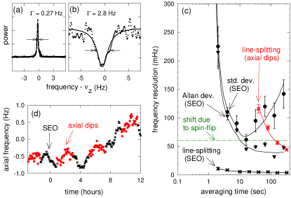
Figure 2: SEO peak (a) and noise dip (b) for 160 s of averaging. (c) Frequency resolution achieved with a single average of an SEO peak (black x) and noise dip (red x), with the standard deviation (black points) and Allan deviation (black triangles) of averaged SEO measurements. (d) Drift of 256 s averages over sixteen night time hours.

The axial frequency is determined to higher precision using the better signal-to-noise and narrower signal width of a one-proton SEO (Fig. 2a). The one-particle SEO, realized previously only with an electron SelfExcitedOscillator , is realized by adjusting the amplitude and phase of the amplified induced signal and feeding this back to the other side of the trap as a driving force on the proton. The feedback produces a force $F_{d}(t)\sim mG\gamma_{z}\dot{z}$ with feedback gain $G$. Self-excitation occurs, in principle, when the feedback cancels the damping at $G=1$. Noise causes amplitude diffusion and energy growth, however, and $G$ slightly different from unity will either decrease or increase $A$ exponentially. A stable and useful SEO thus requires limiting the amplitude to some value $A_{o}$. Here a digital signal processor (DSP) chip Fourier transforms the signal to determine $A$, and makes $G=1+a(A-A_{o})$ SelfExcitedOscillator .

An axial oscillation $z(t)=A\cos(\omega t)$ generates a feedback force $F_{d}(t)=-\omega AGm\gamma_{z}\sin(\omega t+\phi)$, when a phase shift $\phi$ is introduced (Fig. 1). Inserting in Eq. 3 yields

$$G\cos(\phi) = 1$$ (4)

$$G\,\omega\,\gamma_{z}\sin(\phi) = \omega^{2}-\left[\omega_{z}(A)\right]^{2}$$ (5)

For $(\gamma_{z}/\omega_{z})\tan(\phi)<<1$, the SEO thus depends on $\phi$ as

$$\omega(A,\phi)\approx\omega_{z}(A)+\frac{\gamma_{z}}{2}tan(\phi)\;.$$ (6)

With positive feedback, and a feedback phase adjusted to optimize the signal (Fig. 3a), the measured SEO frequency as a function of feedback phase fits well to Eq. 6 (Fig. 3b). The scatter in repeated frequency measurements (Fig. 3c) is reduced when the trapping potential is tuned to make the best possible electrostatic quadrupole.

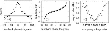
Figure 3: (a) SEO signal strength vs. feedback phase. (b) Measured axial frequency vs. feedback phase (points) fit to the expected Eq. 6. (c) Tuning for optimal SEO stability by adjusting trap anharmonicity.

Sideband cooling, a method to radially center the proton, is especially important given that the magnetic field changes significantly as a function of radial position. A sideband cooling drive at $\omega_{z}+\omega_{-}$, applied across the halves of a compensation electrode (Fig. 1) to produce an $zy$ potential gradient Review , makes the transitions between axial states $k$ and magnetron states $\ell$ indicated by arrows in Fig. 1b. The probability $P_{k,\ell}$ satisfies

$$0=-P_{k,\ell}\,(\Gamma_{+}+\Gamma_{-})+P_{k-1,\ell+1}\,\Gamma_{-}+P_{k+1,\ell-1}\,\Gamma_{+}.$$ (7)

This steady-state rate equation has rates that depend on axial and magnetron raising and lowering operators Review ,

$$\Gamma_{+} \sim |\!<\!k+1,\ell-1|a_{z}^{\dagger}\,a_{-}|k,\ell\!>\!|^{2}\sim(k+1)\ell$$ (8)

$$\Gamma_{-} \sim |\!<\!k-1,\ell+1|a_{z}\,a_{-}^{\dagger}|k,\ell\!>\!|^{2}\sim k(\ell+1).$$ (9)

The axial distribution remains a Boltzmann distribution due to its coupling to the detection resistor, a reservoir at temperature $T_{z}$, so that $P_{k,\ell}=p_{\ell}\,\exp{[-k\hbar\omega_{z}/(k_{B}T_{z})]}$. The solution to Eq. 7 is a magnetron distribution,

$$p_{\ell}\sim\exp{[-\ell\hbar\omega_{-}/(k_{B}T_{m})]},$$ (10)

where the effective magnetron temperature is $T_{m}=T_{z}\omega_{-}/\omega_{z}$. The theoretical cooling limit WinelandFrequencyDivision ; Review ,

$$k_{B}T_{m}=\langle-E_{mag}\rangle=\frac{\omega_{-}}{\omega_{z}}\langle E_{z}\rangle\,=\frac{\omega_{-}}{\omega_{z}}\,k_{B}T_{z},$$ (11)

comes from evaluating the average of the magnetron energy, $\langle E_{mag}\rangle\,=\sum_{\ell}p_{\ell}\,E_{\ell}$, with $E_{\ell}=-(\ell+1/2)\hbar\omega_{-}$. Decreasing $\ell$ increases the potential energy on a radial hill, while decreasing the much smaller kinetic energy, so $E_{\ell}$ is negative. Ref. Review extends the theoretical argument and limit to off-resonant sideband cooling drives.

The outcome of sideband cooling in the trap of Fig. 1a is investigated with a three-step sequence. First, the axial energy is either left in equilibrium with the detection resistor or modified using feedback. Second, a sideband cooling drive at $\omega_{z}+\omega_{-}$ is applied and then turned off. Third, the SEO is started and the axial frequency measured. Each application of sideband cooling produces a measurably different magnetron state and $\omega_{z}(A)$, so the sequence is repeated to make histograms of measured axial frequencies.

The gray histogram and Gaussian fit in Fig. 4a show the scatter for repeated measurements of $\omega_{z}(A)$ taken with no sideband cooling drive (i.e. no change in magnetron radius) and no feedback (i.e. no change in $T_{z}$).

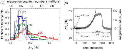
Figure 4: (a) Histograms of magnetron states after no sideband cooling (gray), and produced by sideband cooling using feedback cooling (blue), no feedback (green), and with feedback heating (red). Solid curves are convolutions of the gray Gaussian resolution function and Boltzmann distributions at the specified $T_{z}$. (b) The magnetron radius increase from a sideband drive at $\omega_{z}-\omega_{-}$ is fit to an exponential and extrapolated back to an initial magnetron radius.

Sideband cooling with no feedback broadens the gray into the green histogram (Fig. 4a). A convolution (green curve) of Eq. 10 with $T_{m}=30$ mK (corresponding to $T_{z}=8\pm 2$ K) and the gray Gaussian resolution function fits the measured histogram when Eq. 2 is used to convert magnetron energy to axial frequency shift. The axial temperature is reasonably higher than the $T_{z}=5.2$ K we realized with one electron in a 1.6 K apparatus FeedbackCoolingPRL .

Feedback changes the measured $T_{z}$ as predicted, from $T_{z0}$ at $G$=0 to $T_{z}(G)=(1-G)T_{z0}$ (Fig. 5b), increasing our confidence in this new way to measure the axial temperature. The corresponding damping widths also change just as predicted, from $\Gamma_{z0}$ to $\Gamma_{z}(G)=(1-G)\Gamma_{z0}$ (Fig. 5a). The ratios in Fig. 5c are constant, consistent with the fluctuation-dissipation theorem.

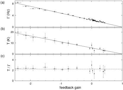
Figure 5: Measured damping widths (a), temperatures (b), and their ratios (c) as a function of the feedback gain, $G$.

Feedback cooling of the axial motion to $T_{z}=4$ K narrows the distribution of magnetron states (blue histogram in Fig. 4a) such that the effective magnetron temperature is $T_{m}=14$ mK. Feedback cooling from $T_{z}=8$ to $4$ K seems plausibly higher than the cooling from 5.2 to 0.85 K FeedbackCoolingPRL achieved with one electron in a 1.6 K apparatus. Feedback heating of the axial motion to $T_{z}=20$ K broadens the distribution (red histogram in Fig. 4a).

A check on the magnetron orbit size produced by sideband cooling comes from expanding the orbit size exponentially with a sideband heating drive at $\omega_{z}-\omega_{-}$ VanDyckMagnetronCoolingLimit ; Review . Each trial (e.g. Fig. 4b) is extrapolated to determine the radius at the start of the heating. Averaging the initial radii from 200 trials gives $11\pm 2~{}\mu\rm{m}$, consistent with $T_{z}=8\pm 2$ K from Fig. 4a, and hence with the theoretical cooling limit (Eq. 11). We do not understand the earlier electron observations VanDyckMagnetronCoolingLimit ; Review but note that progress has been made in the detection electronics that sets $T_{z}$.

Fig. 2c shows that for the first time in a strong magnetic gradient, the resolution achieved in measuring $\omega_{z}$ is comparable to the 60 mHz resolution needed to observe a proton spin flip (for a 16 s averaging time). The resolution is much better for a single SEO measurement (black x) than for a single dip measurement (red x). Repeated SEO frequency measurements have a standard deviation (black points) and an Allan deviation (black triangles) that is larger than the precision for a single measurement. Fluctuations in the trapping potential, mechanical vibrations, temperature variations, and fluctuating contact potentials are being investigated as possible sources of the scatter.

Sideband cooling is required to minimize the scatter and achieve the 60 mHz resolution. However, Fig. 4a demonstrates that an application of sideband cooling randomly selects a new magnetron radius and $\omega_{z}$ that is shifted by much more than this resolution on average. A solution starts with an initial sideband cooling period, after which $\omega_{z}$ is measured. An attempt to make a spin flip can be then made for several minutes, during which time unwanted magnetron heating shifts $\omega_{z}$ typically by about 0.3 Hz/hr (Fig. 2d). Measuring $\omega_{z}$ will thus reveal a shift larger or smaller than 60 mHz depending upon whether the spin has or has not flipped. The process can then be repeated, with cooling selecting a new $\omega_{z}$.

In conclusion, a one-proton self-excited oscillator and one-proton feedback cooling are realized for the first time. A very strong magnetic gradient is added to the Penning trap in which the proton is suspended to make it possible to observe sideband cooling distributions and to investigate the possibility of observing spin flips. Sideband cooling of the undamped proton magnetron motion to 14 mK is demonstrated, even though every application of sideband cooling shifts the monitored SEO oscillation frequency more than would a spin flip. As an application, the SEO oscillation frequency is resolved at the high precision needed to observe a spin flip of a single $\overline{\rm{p}}$ or p, opening a possible new path towards comparing the $\overline{\rm{p}}$ and p magnetic moments at a precision higher than current comparisons by six orders of magnitude or more.

Thanks to the NSF AMO program, the AFOSR, the NDSEG, and the Humboldt Foundation for support.

References

- (1) B. D’Urso, R. Van Handel, B. Odom, D. Hanneke, and G. Gabrielse, Phys. Rev. Lett. 94, 113002 (2005)
- (2) B. D’Urso, B. Odom, and G. Gabrielse, Phys. Rev. Lett. 90, 043001 (2003)
- (3) D. Hanneke, S. Fogwell, and G. Gabrielse, Phys. Rev. Lett. 100, 120801 (2008)
- (4) W. Quint, J. Alonso, S. Djekić, H.-J. Kluge, S. Stahl, T. Valenzuela, J. Verdú, M. Vogel, and G. Werth, Nucl. Inst. Meth. Phys. Res. B 214, 207 (2004)
- (5) G. Werth, J. Alonso, T. Beier, K. Blaum, S. Djekic, H. Häffner, N. Hermanspahn, W. Quint, S. Stahl, J. Verdú, T. Valenzuela, and M. Vogel, Int. J. Mass Spectrom. 251, 152 (2006)
- (6) R. Van Dyck, Jr., P. Ekstrom, and H. Dehmelt, Nature 262, 776 (1976)
- (7) L. S. Brown and G. Gabrielse, Rev. Mod. Phys. 58, 233 (1986)
- (8) R. Blatt and D. J. Wineland, Nature 453, 1008 (2008)
- (9) T. Rosenband, D. B. Hume, P. O. Schmidt, C. W. Chou, A. Brusch, L. Lorini, W. H. Oskay, R. E. Drullinger, T. M. Fortier, J. E. Stalnaker, S. A. Diddams, W. C. Swann, N. R. Newbury, W. M. Itano, D. J. Wineland, and J. C. Bergquist, Science 319, 1808 (2008)
- (10) H. Perrin, A. Kuhn, I. Bouchoule, and C. Salomon, Europhys. Lett. 42, 395 (1998)
- (11) T. Rocheleau, T. Ndukum, C. Macklin, J. B. Hertzberg, A. A. Clerk, and K. C. Schwab, Nature 463, 72 (2010)
- (12) D. J. Wineland, J. Appl. Phys. 50, 2528 (1979)
- (13) R. S. Van Dyck, Jr., P. B. Schwinberg, and H. G. Dehmelt, “New frontiers in high energy physics,” ((Plenum, New York), 1978) p. 159
- (14) H. Häffner, T. Beier, S. Djekić, N. Hermanspahn, H.-J. Kluge, W. Quint, S. Stahl, J. Verdú, T. Valenzuela, and G. Werth, Eur. Phys. J. D 22, 163 (2003)
- (15) S. Djekic, J. Alonso, H.-J. Kluge, W. Quint, S. Stahl, T. Valenzuela, J. Verdú, M. Vogel, and G. Werth, Eur. Phys. J. D. 31, 451 (2004)
- (16) G. Gabrielse, X. Fei, L. A. Orozco, R. L. Tjoelker, J. Haas, H. Kalinowsky, T. A. Trainor, and W. Kells, Phys. Rev. Lett. 65, 1317 (1990)
- (17) G. Gabrielse, L. Haarsma, and S. L. Rolston, Intl. J. of Mass Spec. and Ion Proc. 88, 319 (1989), ibid. 93, 121 (1989)
- (18) G. Gabrielse, D. Phillips, W. Quint, H. Kalinowsky, G. Rouleau, and W. Jhe, Phys. Rev. Lett. 74, 3544 (1995)
- (19) D. J. Wineland and H. G. Dehmelt, J. Appl. Phys. 46, 919 (1975)