What Lies Beneath: Using p(z) to Reduce Systematic Photometric Redshift Errors

Abstract

We use simulations to demonstrate that photometric redshift “errors” can be greatly reduced by using the photometric redshift probability distribution $p(z)$ rather than a one-point estimate such as the most likely redshift. In principle this involves tracking a large array of numbers rather than a single number for each galaxy. We introduce a very simple estimator that requires tracking only a single number for each galaxy, while retaining the systematic-error-reducing properties of using the full $p(z)$ and requiring only very minor modifications to existing photometric redshift codes. We find that using this redshift estimator (or using the full $p(z)$) can substantially reduce systematics in dark energy parameter estimation from weak lensing, at no cost to the survey.

1. Introduction

Photometric redshifts (Connolly et al. 1995, Hogg et al. 1998, Benitez 2000) are a key component of galaxy surveys. As surveys get larger, reducing statistical uncertainties, systematic errors become more important. Systematic errors in photometric redshifts are therefore a top concern for future large galaxy surveys, for example as highlighted by the Dark Energy Task Force (Albrecht et al. 2006).

Much of the concern has centered on “catastrophic outliers” which are galaxies for which the photometric redshift is very wrong, for example when mistaking the Lyman break at $z\sim 3$ for the 4000Å break at very low redshift. Even a small fraction of outliers can significantly impact the downstream science, and modeling this impact requires going beyond simple Gaussian models of photometric redshift errors.

In many cases, however, outliers are “catastrophic” only because they have a multimodal redshift probability $p(z)$, which cannot be accurately represented by a single number such as the most probable redshift. Fernandez-Soto et al. (2002) showed that after defining confidence intervals around the $p(z)$ peaks, 95% of galaxies in their sample had spectroscopic redshifts within the 95% confidence interval and 99% had spectroscopic redshifts within the 99% confidence interval. Yet the same data appear to contain catastrophic outliers on a plot where each galaxy is represented only by a point with symmetric errorbars.

There is a second motivation for using the full $p(z)$. The redshift ambiguities described above are due to color-space degeneracies. But even without these degeneracies, photometric redshift errors should be asymmetric about the most probable redshift due to the nonlinear mapping of redshift into color space. Avoiding biases from this effect also requires reference to $p(z)$. Indeed, Mandelbaum et al. (2008) showed that using $p(z)$ in Sloan Digital Sky Survey (SDSS) data (which are not deep enough to suffer serious degeneracies) substantially reduced systematic calibration errors for galaxy-galaxy weak lensing.

In this paper we demonstrate, using simple simulations, the reduction in systematic error that can result from using the full $p(z)$ in a deep survey with significant degeneracies. We also introduce a simple way to reduce the computational cost of doing so.

2. Simulations

We conducted simulations similar to those in Margoniner & Wittman (2008) and Wittman et al. (2007), which used the Bayesian Photometric Redshift (BPZ, Benitez 2000) code, including its set of six template galaxy spectral energy distributions (SEDs) and its set of priors on the joint magnitude-SED type-redshift distribution. We started with an actual R band catalog from the Deep Lens Survey (DLS, Wittman et al. 2002). For each galaxy, we used the $R$ magnitude to generate a mock type and redshift according to the priors, and then generated synthetic colors in the BVRz^′ filter set used by DLS. (The filter set is not central to the argument here, but one must be used for concreteness.) We then added photometry noise and zero-point errors representative of the DLS. The color distributions in the resulting mock catalog were similar to those of the actual catalog, indicating that the mock catalog is consistent with a real galaxy survey.

We then ran the mock catalog of 83,000 galaxies through BPZ, saving the full $p(z)$. In a post-processing stage, we can extract from the full $p(z)$ not only the most probable redshift (which had already been determined by BPZ and labeled $z_{B}$), but other candidate one-point estimates such as the mean and median of $p(z)$, as well as the summed $p(z)$ for any desired set of galaxies.

3. Results

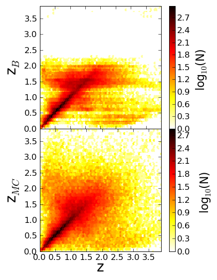
We first show one of the traditional one-point estimates to more clearly illustrate the problem. The left panel of Figure 1 shows the most probable redshift $z_{B}$ vs. true redshift $z$. To accurately render both the high- and low-density parts of this plot, we show it as a colormap rather than a scatterplot. The core is rather tight, requiring a logarithmic mapping between color and density to bring out the more subtle features in the wings. With this mapping, the systematics are clear: a tendency to put galaxies truly at $z\sim 2-3$ at very low redshift; a tendency to put galaxies truly at low redshift at $z_{B}\sim 1.4-2$; and asymmetric horizontal smearing in several different $z_{B}$ intervals, e.g. at $z_{B}\sim 1.5$. The specifics of the features depend on the filter set, but their general appearance is typical (but note that they will be difficult to see in plots based on spectroscopic followup of deep imaging surveys, as the brighter, spectroscopically accessible, galaxies form a much tighter relation). Corresponding plots are not shown for other one-point estimates such as the mean and median of $p(z)$, but they have similar to worse systematic deviations.

Which systematics are most important depends on the application. In this paper we consider two-point correlations of weak gravitational lensing (cosmic shear), which require that the photometric redshift distribution of a sample of galaxies be as close as possible to the true redshift distribution; errors on specific galaxies are not important. Also, accurate knowledge of the scatter is much more important than minimizing the amount of scatter. Thus, Figure 1 would ideally be symmetric about a line of unity slope, reflecting the fact that the photometric and true redshift distributions are identical. This is clearly not the case for the top panel of Figure 1.

Figure 1.— Top: each galaxy’s most probable photometric redshift ($z_{B}$) vs. spectroscopic redshift. Bottom: Monte Carlo sampling from each galaxy’s redshift probability distribution ($z_{MC}$) vs. spectroscopic redshift. Sampling the distribution cleans up many artifacts introduced by considering only the most probable photometric redshift.

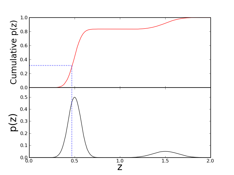
Ideally $p(z)$ contains the required information lacking in the single number $z_{B}$, but it is also more difficult to work with, requiring the storage and manipulation of an array of numbers for each galaxy. We simplify the computational bookkeeping by defining a single number which is by construction representative of the full $p(z)$. This estimate is simply a random number distributed according to the probability distribution $p(z)$ and is denoted by $z_{MC}$ because it is a Monte Carlo sample of the full $p(z)$. Specifically, for each galaxy, a random number $x$ is drawn uniformly from the interval $[0,1)$, and the Monte Carlo redshift $z_{MC}$ is defined such that $\int_{0}^{z_{MC}}p(z^{\prime})dz^{\prime}=x$. Figure 2 illustrates the process. The bottom panel shows $p(z)$ as usually plotted, while the top panel shows the cumulative $p(z)$, that is, the probability that the galaxy lies at redshift less than the value on the abscissa. A random number in the range 0-1 is drawn, in this case 0.32, and the redshift at which the cumulative $p(z)$ has a value of 0.32 (dotted line) is recorded as $z_{MC}$, in this case 0.47. This results in a single number for each galaxy, which remains unbiased even if $p(z)$ is multimodal and/or asymmetric. Of course, some precision is lost in this process; it should be avoided when studying a small number of galaxies in great detail, but for large samples of galaxies it must converge to the $p(z)$ of the sample. Furthermore, it requires only a minor modification to most photometric redshift codes.

Figure 2.— Construction of the $z_{MC}$ estimator for an example galaxy. The bottom panel shows $p(z)$ as usually plotted. The top panel shows the cumulative $p(z)$, that is, the probability that the galaxy lies at redshift less than the value on the abscissa. A random number in the range 0-1 is drawn, in this case 0.32, and the redshift at which the cumulative $p(z)$ has a value of 0.32 is recorded as the Monte Carlo estimate $z_{MC}$.

The bottom panel of Figure 1 shows $z_{MC}$ vs. $z_{B}$. Clearly, the systematics are vastly improved. Even with the logarithmic scaling, it is difficult to see departures from symmetry about a line of unity slope. We therefore compare one-dimensional histograms in what follows. A typical use of photometric redshifts in a galaxy survey will be to bin the galaxies by redshift, for example to compute shear correlations in redshift shells. Because the true redshifts will not be known, the galaxies must be binned by some photometric redshift criterion. For simplicity, we choose $z_{B}$.

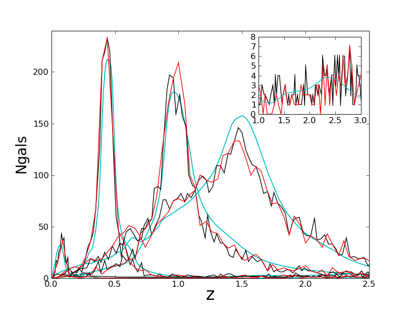
Figure 3 (upper panel) shows true and inferred redshift distributions of galaxies in four $z_{B}$ bins: 0-0.1, 0.4-0.5, 0.9-1.1, and 1.4-1.6. The true distributions is shown in black, the distribution inferred from $z_{MC}$ is shown in red, and the distribution inferred from summing the galaxies’ $p(z)$ is shown in blue. The asymmetry and the wings of the true redshift distribution are well captured by $z_{MC}$ or by summing $p(z)$. By comparison, using each galaxy’s most probable redshift $z_{B}$ to infer the redshift distributions would have resulted in four vertical-sided bins, which would become roughly Gaussian after convolving with the typical galaxy’s $z_{B}$ uncertainty. It is clear that this would not capture the true redshift distribution nearly as well as the $p(z)$ method does. For example, the inset in Figure 3 shows a small high-redshift ($z\sim 2.5$) bump in the 0.4-0.5 bin which is captured by $z_{MC}$ or by summing $p(z)$. Looking only at the most probable redshift $z_{B}$ would result in these galaxies being considered catastrophic outliers.

Figure 3.— Black: true redshift distributions of photometric redshift cuts $z_{B}<0.1$, 0.4-0.5, 0.9-1.1, and 1.4-1.6 in the simulation. Red: distributions of the $z_{MC}$ estimator for the same sets of galaxies. Blue: summed $p(z)$ for the same sets of galaxies. The simple estimator $z_{MC}$ does as well as tracking the full $p(z)$. Using each galaxy’s most probable redshift $z_{B}$ to infer the redshift distributions would result in four vertical-sided bins. Inset: a high-redshift bump in the true redshift distribution of galaxies with $0.4<z_{B}<0.5$ is captured by the summed $p(z)$ or by $z_{MC}$, but would be considered “catastrophic outliers” if $z_{B}$ were used.

Another way to reduce “catastrophic outliers” and related systematics might be to discard galaxies whose $p(z)$ is multimodal, not sharply peaked, or otherwise fails some test. This may be effective, but it greatly reduces the number of galaxies available to work with. The $z_{MC}$ and full $p(z)$ methods accurately reflect the true redshift distributions without requiring any reduction in galaxy sample size. This is important for applications such as lensing, for which galaxy shot noise will always be an issue.

Having demonstrated that using $p(z)$ (whether by sampling or by using the full distribution) greatly reduces photometric redshift systematics, two questions naturally arise. How much better is it in terms of a science-based metric? And what are the remaining errors or limitations? Because $z_{MC}$ and the full $p(z)$ give very similar results, references to using $p(z)$ in the remainder of the paper should be understood to include either implementation.

4. Effect on Dark Energy Parameter Estimation

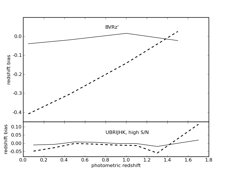
For each of the four $z_{B}$ bins shown in Fig. 3, we compute the redshift bias (inferred minus true mean redshift) for the full $p(z)$ and $z_{B}$ approaches. These are shown in Fig. 4 as the solid and dotted lines respectively (the results for $z_{MC}$ are nearly indistinguishable from those for the full $p(z)$ and are not shown). For the DLS filter set and noise model, the bias is within a few hundredths of a unit redshift when using $p(z)$, but only within several tenths when using the most probable redshift $z_{B}$. For lensing applications, the $z_{B}$ bias at low redshift is exaggerated somewhat, because it results from a small outlying bump at high redshift, as shown in the inset of Fig. 3. In a real survey, these high-redshift interlopers would be smaller and fainter than the galaxies that really belong in the low-redshift bin, and therefore have less precise shape measurements and smaller weight on the shear statistics. We account for this effect by assigning a lensing weight to each mock galaxy based on its magnitude and drawn from the actual distribution of weights as a function of magnitude in the DLS. This reduces the bias of the lowest-redshift bin to 0.02 for $p(z)$ and 0.24 for $z_{B}$, and has a progressively smaller effect on higher-redshift bins.

Figure 4.— Redshift bias (inferred minus true mean redshift) for the four bins shown in Fig. 3, when using the full $p(z)$ (solid) and when using the most probable redshift $z_{B}$ for each galaxy (dotted). The results for $z_{MC}$ are nearly indistinguishable from those for the full $p(z)$ and are not shown. Top panel: BVRz^′ filter set and DLS noise model. Bottom panel: UBRIJHK filter set and optimistic noise model with photometric signal-to-noise of 10 in each filter, regardless of redshift or magnitude.

Fig. 7 of Ma et al. (2006) shows the degradation in dark energy parameters for a wide and very deep weak lensing survey, as a function of the tightness of priors that can be put on the redshift bias and scatter in photometric redshift bins. It shows that loose priors of order 0.2 result in 80-85% degradation in $w_{0}$ estimates (with respect to a survey with absolutely no redshift errors). If, on the other hand, one need only allow for a $\sim 0.02$ bias as with the $p(z)$ approach, the degradation decreases to 50-60%. For estimating $w_{a}$, the degradation decreases from a factor of six to a factor of about 2.5 by employing $p(z)$.

These are only rough estimates, for a number of reasons. Future surveys as deep as those contemplated by Ma et al. (2006) will use more extensive filter sets, which will probably improve the $z_{B}$ performance somewhat with respect to the $p(z)$ performance. And nearer-term, shallower surveys have looser redshift requirements because their shear measurements are not as precise. But it is clear that using $p(z)$ greatly improves the survey at essentially no cost. We also conducted simulations using a more extensive filter set, to check the generality

5. Remaining Errors and Limits of this Work

The simulations are simplistic in that the same six SED templates (and priors) used to infer $p(z)$ are used to generate the mock catalogs. In real photometric redshift catalogs, $p(z)$ will be less perfect because galaxy SEDs are more varied and priors are imperfectly known. Smaller effects of the same nature include uncertainties in real-life filter and throughput curves, which are artificially reduced to zero here. However, these errors also affect the most probable redshift. Therefore, although the simulated results presented here are optimistic overall (given this filter set), the performance of $p(z)$ relative to using the most probable redshift may not be. More sophisticated simulations beyond the scope of this paper will be required to determine the limits of $p(z)$ accuracy for any given filter set and survey depth.

The remaining redshift bias is not trivial, 0.01-0.02. This is an order of magnitude larger than required to keep the $w_{0}$ degradation within 10% of an ideal survey (for the deepest surveys; requirements are less stringent for shallower surveys). However, a few factors are actually pessimistic here compared to future large surveys: the limited filter set, and relatively large zeropoint errors ($\sim 0.03$ mag here vs 0.01 mag for SDSS and future large surveys). A more extensive filter set will improve both the $p(z)$ and the $z_{B}$ etimates, but will probably improve the $z_{B}$ estimate more as it eliminates some degeneracies. Again, survey-specific simulations will be required to make more specific conclusions.

Finally, there is a source of bias not simulated here: Eddington (1913) bias. The type and redshift priors are based on magnitude, but at the faint end magnitudes are biased due to the asymmetry between the large number of faint galaxies that noise can scatter to brighter magnitudes, versus the smaller number of moderately bright galaxies that noise can scatter to fainter magnitudes. Surveys wishing to derive photometric redshifts for galaxies detected at, say, 10$\sigma$ or fainter, must use the Hogg & Turner (1998) prescription for removing Eddington bias from each galaxy’s flux measurements if they are to avoid nontrivial systematic errors.

6. Summary

We have shown that using the photometric redshift probability distribution $p(z)$ greatly reduces photometric redshift systematic errors, as compared to using a simple one-point estimate such as the most probable redshift or the mean or median of $p(z)$. Various authors have made similar points previously, particularly Fernandez-Soto et al. (2002), who wrote that “this information [p(z)] can and must be used in the calculation of any observable quantity that makes use of the redshift.” However, adoption of this practice has been slow to nonexistent, even among authors who are aware of the point, because it is cumbersome to track a full $p(z)$ for each galaxy. We have shown that a very simple modification to photometric redshift codes, namely choosing a Monte Carlo sample from the $p(z)$, produces a single number for each galaxy which greatly reduces the systematic errors compared to using any other one-point estimate such as the mean, median, or mode of $p(z)$. In contrast to approaches which simply reject galaxies which could be outliers, this method can make use of every galaxy in a survey. We have shown that this method results in substantial improvements in a flagship application, estimating dark energy parameters from weak lensing, at no cost to the survey.

References

- Albrecht et al. (2006) Albrecht, A., et al. 2006, arXiv:astro-ph/0609591
- (2) Benitez, N. 2000, ApJ, 536, 571
- Connolly et al. (1995) Connolly, A. J., Csabai, I., Szalay, A. S., Koo, D. C., Kron, R. G., & Munn, J. A. 1995, AJ, 110, 2655
- Eddington (1913) Eddington, A. S. 1913, MNRAS, 73, 359
- Fernández-Soto et al. (2002) Fernández-Soto, A., Lanzetta, K. M., Chen, H.-W., Levine, B., & Yahata, N. 2002, MNRAS, 330, 889
- Hogg & Turner (1998) Hogg, D. W., & Turner, E. L. 1998, PASP, 110, 727
- Hogg et al. (1998) Hogg, D. W., et al. 1998, AJ, 115, 1418
- Huterer et al. (2006) Huterer, D., Takada, M., Bernstein, G., & Jain, B. 2006, MNRAS, 366, 101
- Ma et al. (2006) Ma, Z., Hu, W., & Huterer, D. 2006, ApJ, 636, 21
- Mandelbaum et al. (2008) Mandelbaum, R., et al. 2008, MNRAS, 386, 781
- Margoniner & Wittman (2008) Margoniner, V. E., & Wittman, D. M. 2008, ApJ, 679, 31
- Wittman et al. (2002) Wittman, D. M., et al. 2002, Proc. SPIE, 4836, 73
- Wittman et al. (2007) Wittman, D., Riechers, P., & Margoniner, V. E. 2007, ApJ, 671, L109