Lyapunov stability of Vlasov Equilibria using Fourier-Hermite modes
Abstract
We propose an efficient method to compute Lyapunov exponents and Lyapunov eigenvectors of long-range interacting many-particle systems, whose dynamics is described by the Vlasov equation. We show that an expansion of a distribution function using Hermite modes (in momentum variable) and Fourier modes (in configuration variable) converges fast if an appropriate scaling parameter is introduced and identified with the inverse of the system temperature. As a consequence, dynamics and linear stability properties of many-particle states, both in the close-to and in the far-from equilibrium regimes can be predicted using a small number of expansion coefficients. As an example of a long-range interacting system we investigate stability properties of stationary states of the Hamiltonian mean-field model.
pacs:
52.65.Ff,05.10.-a,02.70.DhI Introduction
Neglecting particle correlations, the collective dynamics of many-particle systems interacting via long-range forces obeys the Vlasov equation jeans1915mnras ; vlasov1961 ; bohm1949 ; balescu1997 :
| (1) |
Here is the single-particle density function, while and are, respectively, the particle configuration and momentum coordinates. The long-range force is generated by the self-field
| (2) |
where is the particle interaction potential, and is the particle density.
There is growing evidence that the evolution of many-particle systems with long-range interactions lends itself to interpretation in terms of trajectories that trace a finite repertoire of collective patterns with abrupt transitions between them, thus corroborating the claim, stating that only a few effectively active degrees of freedom partake in dynamics of such systems, despite the huge dimensionality of the many-particle state space.
Presence of transitions indicates also the relevance of nonlinear dynamical effects: instabilities, which have the capacity to strongly alter the state of a system, even before a gradual thermalization of the particles. Analysis of a dynamical system in terms of the properties of its invariant structures (equilibria, manifolds, invariant orbits) has been established as a fruitful approach to gaining insights into the nonlinear evolution of a system poincare . In particular, the stable equilibria can be identified with relevant collective patterns, the hyperbolic manifolds of the unstable equilibria with pathways of transitions. With the information about the Lyapunov spectrum and Lyapunov eigenvectors of such collective patters, control of the systems is feasible.
Effective representation of the equilibria and of their local Lyapunov stability properties are one of the main challenges addressed in this Paper. Focusing on one-dimensional systems represented by density functions with Gaussian-like tails in the momentum variable and spatially periodic boundary conditions in the configuration variable, we demonstrate that a Fourier-Hermite expansion of can reproduce both the Lyapunov spectrum and Lyapunov eigenvectors with a small number of expansion coefficients. We also show that introduction of an appropriate scaling parameter, to be identified with the inverse of the system temperature, allows to improve the convergence of an expansion.
As a test model, we investigate Lyapunov stability properties of stationary states of the Hamiltonian mean-field (HMF) model longrangebook2002 ; inagaki1993 ; antoni1995 ; yamaguchi2004 ; morita2006 ; barre2006physa ; antoniazzi2007pre ; latora1999 ; yamaguchi2007 ; antoniazzi2007prl1 ; chavanis2007epj . Prior studies of the HMF model have revealed non-trivial collective oscillations morita2006 and thermodynamical properties that pertain to a large class of long-range interacting systems yamaguchi2004 ; barre2006physa ; antoniazzi2007pre ; latora1999 ; yamaguchi2007 ; antoniazzi2007prl1 .
The plan of the Paper is as follows. In Sec. II we introduce the Fourier-Hermite expansion of a density function and discuss the scaling parameter. The spectral equation, the Lyapunov spectrum and Lyapunov eigenvectors are introduced in Sec. III. Relevant facts about the HMF model are summarized in Sec. IV. Results, obtained from the application of our method to the HMF model, are presented in Sec. V. Finally, in Sec. VI, we draw conclusions.
II The Fourier-Hermite expansion
In the following, we focus on one dimensional systems. Collective properties of many-particle dynamical systems are typically more evident when the system states are represented in terms of density functions. Further discretization of a density function in terms of a finite set of coefficients provides an alternative representation of the system with, hopefully, few couplings among different s. The latter step can be formalized, stating that the density function is a linear map of the coefficients , given by
| (3) |
A Galerkin projection fornberg1995 of a density function to a set of coefficients is an example of such a map. For the Vlasov equation, discretization in momentum variable commands careful analysis. Therefore we first consider a partial projection of :
| (4a) | ||||
| (4b) | ||||
Here are basis functions, and are basis weights. They constitute complete, normalized, adjoint bases, i.e. . We have introduced a free scaling function , which will be determined later. The parameter will be fixed by requiring that .
In the following, we make use of the so-called asymmetrically weighted Hermite expansion schumer1998 ; armstrong1967 ; grant1967 (as opposed to the symmetrically weighted Hermite expansion, discussed in schumer1998 ), defined by
| (5a) | ||||
| (5b) | ||||
Analysis of the Vlasov equation based on Hermite expansions in momentum variable has been introduced in armstrong1967 ; grant1967 , with the emphasis on the accuracy of numerical solvers.
Advantages of Hermite polynomials include facts that the basis functions decay as for large , i.e. in accordance with typical physical boundary conditions, and that the recursion relations, relevant to the Vlasov equation, are simple:
| (6a) | ||||
| (6b) | ||||
In general, the density can be expressed as , where , . In the asymmetrically weighted Hermite expansion . Looking at (2), one can see that in this way the couplings between different momentum modes are minimal. This fact motivates the choice of the asymmetrically weighted expansion, whose recursion coefficients are , , , , .
Using the expansion (4), the Vlasov equation (1) is cast as
| (7) |
where are defined as
| (8) |
and
| (9) |
Here .
The Vlasov dynamics typically proceeds as an interplay between two mechanisms, the advection and the convection, and associated with them there are two scales of spatial variations. The convection, represented by the nonlinear term in (1), determines the evolution of the width of the distribution function in momentum variable. It is related to the (time-dependent) system temperature :
| (10) |
On this scale, transitions between different macroscopic states can be observed. The advection term drives the filamentation process independently. It is characterized by ever-thinning of inhomogeneities (filaments) of , down to the scale of fluctuations in the underlying discrete many-particle system.
In order to represent large-scale variations of efficiently, we focus on the former, the temperature scale. The parameter in the expansion (4) can be tuned to maximize the content of the lowest order mode , assumed to be nonzero. Using (4), one can show that the previous condition is equivalent to
| (11) |
which in turn corresponds to . In this way becomes a dynamical variable, whose evolution is defined by enforcing (11). However, for the Lyapunov exponents of a stationary state, derivatives of , and the two last terms in (7), can be neglected.
In the rest of this paper we will study the Lyapunov spectrum of smooth distributions with periodic boundary conditions in , therefore a Fourier decomposition of is adequate:
| (12) |
With expansions (4) and (12), the system evolution is determined by the complex coefficients , where . The Vlasov matrix can be extended to include the expansion in , by noting that the derivative , acting on , is a diagonal operator: .
For calculations, we use a finite truncation in complex coefficients, and let and .
III Local Lyapunov Exponents
The local Lyapunov spectrum and the corresponding Lyapunov vectors of a stationary state are defined by all solutions (,) of the spectral equation
| (13) |
Here is the fundamental matrix, defined by
| (14) |
On a short time scale, the evolution of a perturbed state (where is a small arbitrary parameter and an arbitrary vector) can be written as , to the first order in . The vector evolves according to the following equation:
| (15) |
Here is the adjoint basis to , satisfying . If for some , , the corresponding eigenvector is amplified exponentially in time. It is therefore referred to as an expanding eigenvector. The expansion rate is called the local Lyapunov exponent. The small number of local Lyapunov exponents is, as a rule, a signature of effective low-dimensionality. The leading local Lyapunov exponent is defined by
| (16) |
It controls the rate of exponential divergence in time of initially proximate states. The divergence is approximated by
| (17) |
where and are the expanding eigenvector and its adjoint, respectively, corresponding to the spectral eigenvalue with . If all are real, the state is said to be spectrally stable.
The rate of exponential divergence between two distribution functions is computed by monitoring the evolution of their difference. This requires the introduction of the concept of the distance between two distribution functions. We define the distance as
| (18) |
IV The HMF model
IV.1 Equations of Motion
The Hamiltonian mean-field (HMF) model longrangebook2002 ; inagaki1993 ; antoni1995 is a continuous time model of a one-dimensional “gas” of globally coupled particles on a circle, with coordinates , momenta and the “magnetization” . The mean magnetization is defined by , where . The HMF Hamiltonian is
| (19) |
It determines the particle evolution by
| (20) |

In the limit , fixed energy per particle ,
| (21) |
correlations between particles yield to collective phenomena. In this, collisionless limit, the Vlasov equation for the HMF assumes the form
| (22) |
where is the single-particle distribution function. The mean-field magnetization is defined by .
IV.2 Homogeneous Stationary States
We consider a two-parameter family of homogeneous () distributions , given by
| (23) |
This distribution is a special case of a class of distributions, defined by , shown to be important in the statistical treatment of the “violent relaxation” processes lynden-bell1967 . Their relevance to the HMF model has been discussed in antoniazzi2007pre .
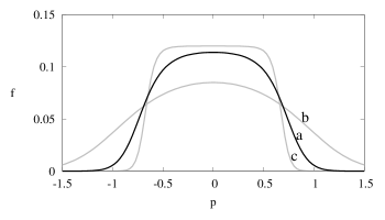
Assuming that is normalized, , the parameters , are related to , by the self-consistency conditions chavanis2007epj : , . Three examples of with different values of are shown in Fig. 1.
The effective temperature , determined by (11), is
| (24) |
where
are the standard Fermi-Dirac integrals.

In Ref. chavanis2007epj , it has been demonstrated that, in the parameter plane (, ), the stable and the unstable stationary states (23) are separated by the boundary curve . Defining for and by
| (25) |
we express as
| (26) |
In Ref. chavanis2007epj it has also been demonstrated that for a fixed value of , . This defines the limiting boundary curve . Note that approaching corresponds to taking the asymptotic limit of of the distribution function (23). In this limit tends to the “water-bag” distribution, defined by , where is the Heaviside function. Close to this boundary, differentiability properties of deteriorate, and the convergence of the coefficient expansion is slower.


In the following we will compare our calculations of Lyapunov exponents with results on phase transitions for the HMF model, discussed in Ref. antoniazzi2007pre ; chavanis2007epj .
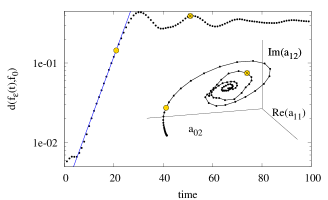
Figure 2 shows the divergence from an equilibrium of a perturbed homogeneous stationary state, corresponding to the curve (a) in Fig. 1. The evolution has been obtained by integrating (20). The initial exponential divergence is clearly displayed, together with the subsequent saturation to a quasi stationary state, characterized by low-frequency oscillations. The inset of Fig. 2 shows the system dynamics, projected in coefficients (,,). As it can be seen, the stretch of the (almost linear) initial trajectory, slightly bending towards the attractor just before the reference point at , shows the qualitative features of the long-term dynamics.
V Results and Discussion
Linearization of the Vlasov Equation (1) around the family of distributions (23) shows that the Lyapunov spectrum comprises a continuum of real eigenvalues, associated with spectrally stable modes, as well as a finite number of imaginary eigenvalues, to be associated with unstable collective modes. In the case of homogeneous distributions, Lyapunov exponents of the collective modes can be expressed succinctly, using the plasma dispersion function , as an equation bohm1949 ; balescu1997 . The plasma dispersion function for the HMF model has been derived in antoni1995 :
| (27) |
where is given by (23). The boundary between stable and unstable stationary states is determined by . The result is the curve , given by (26).
The local (real and positive) Lyapunov exponent is found as a solution of . We define this solution as the Lyapunov map:
| (28) |
where is the inverse of (given by (25)) with respect to the variable , while and are expressed in terms of and using the self-consistency conditions.
For non-homogeneous stationary distributions, the dispersion relation does not have a closed form, such as (27), and solving (13) is the only direct way to obtain the Lyapunov spectrum. Equation (13) specialized for the HMF model reads
| (29) |

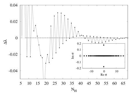
Figure 3 shows the difference between the Lyapunov exponent (16), and the exact value, given by (28), as a function of the truncation order in Hermite polynomials. The number of Fourier modes is fixed at . Two cases are shown, corresponding to the unstable state (a) (exact value ) and to the stable state (b) (), in Fig. 1. As it can be seen, allows to predict real Lyapunov spectrum of the stationary state (b), and to predict a positive Lyapunov exponent of the unstable stationary state (a) qualitatively. Given that the sources of errors include both the finite truncation error, and errors in the approximation of the coefficients (computed using Monte-Carlo integration), the convergence to the exact value can be considered as satisfactory. The inset of Fig. 3 shows the complete Lyapunov spectrum of the unstable state (a), including a single local Lyapunov exponent. All remaining eigenvalues have a vanishing imaginary part and tend to cover the real axis densely.
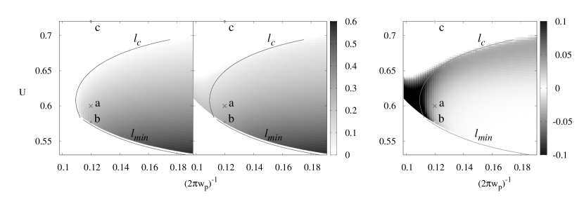
In Fig. 4 we display the Lyapunov map . The exact map (28), the approximation computed via (29), and their difference are shown in the left, center and right panels, respectively. The center panel was computed by averaging the largest Lyapunov exponent over the order of truncation, , between and , and with the fixed . The agreement is fully satisfactory for the high-energy stable stationary states. Indeed, consistently with what is reported in Fig. 3, we have verified that for the computed by (29) Lyapunov spectrum in this region is always real, and therefore predictions of spectral stability are unambiguous. Similarly, apart from the region close to the intersection between and , one can see that also the unstable states are predicted unambiguously. The largest Lyapunov exponent converges to the exact value as the truncation size is increased. As for the error in the intersection region, analysis, similar to the one shown in Fig. 3, demonstrates that close to the prediction of is more sensitive to errors in the coefficients . Moreover, deterioration of results computed with a fixed truncation order close to can be anticipated because of differentiability properties of .

For comparison, the exact Lyapunov exponent for the state (a) . Simulation of one million particles (see Fig. 2) gives . The convergence to of the calculation based on Fourier-Hermite expansion is displayed in Fig. 3. On can see that our method is in good agreement with both the -particle simulation and the exact calculation.
The full solution of (13) provides detailed information about local directionality of transitions associated to each eigenvalue. In the presence of a single positive local Lyapunov exponent, or if one local Lyapunov exponent is larger than the remaining ones, this directionality is expressed by (17). To test accuracy of our method with respect to calculation of expanding eigenvectors, in Fig. 5 we explore the temporal divergence of a perturbed stationary state (a). The distribution function, obtained by directly integrating (20) up to , to near the breakdown of the regime of exponential divergence (see Fig. 2), is displayed in the left panel of Fig. 6. Subtraction of the initial state from the latter is shown in the central panel. A direct comparison with the unstable expanding mode, calculated using truncated (29) with , (see the right panel), demonstrates that also Lyapunov eigenvectors are predicted accurately.
As a final step, we tested the ability of the method to predict the distribution function after the exponential regime, i.e. outside the limit of validity of (29). Results are summarized in Fig. 6. Considering again the perturbed stationary state (a), the distribution function at is shown in the left panel of Fig. 6 (indicated by a thick crossed circle in Fig. 2.) The effective temperature of the distribution is . The difference between a representation using fixed low-order truncation (, ) is shown in the center panel with , and in the right panel with . As it can be seen, the case in which is tuned at the inverse of the system temperature results in smaller errors of the approximation. The agreement using a detuned can be improved by increasing the order of the Hermite expansion.
VI Conclusions
We have proposed an efficient method to compute Lyapunov exponents and Lyapunov eigenvectors of collective states in long-range interacting many-particle systems, whose dynamics is described by the Vlasov equation. The method is based on expanding the distribution function in a Fourier-Hermite basis, with a scaled momentum variable. Having tuned the scaling parameter to maximize the content of the lowest order coefficient of the expansion, we have demonstrated that the Lyapunov exponent and Lyapunov eigenvectors converge fast to the values predicted by direct many-particle simulations and by the exact analytical formula. In the last part of the paper, the ability of the method to predict the evolution of the distribution function in the far-from-equilibrium regime has been demonstrated. As an example of a long-range interacting system, the Hamiltonian mean-field model has been considered. In this context, stability properties of a two-parameter family of homogeneous distributions over a wide range of dynamical conditions has been investigated. Our conclusion is that linear stability properties and collective aspects of dynamics of the HMF model can be represented and computed using a small number of modes, and thus a small numerical effort.
References
- (1) J. H. Jeans. On the theory of star-streaming and the structure of the universe. Mon. Not. R. Astron. Soc., 76(1):70–84, 1915.
- (2) A. Vlasov. Many-particle theory and its application to plasma. Gordon and Breach, New York, 1961.
- (3) D. Bohm and E. P. Gross. Theory of plasma oscillations. A. Origin of medium-like behavior. Phys. Rev., 75(12):1851–1864, 1949.
- (4) R. Balescu. Statistical dynamics: matter out of equilibrium. Imperial College Press, London, 1997.
- (5) H. Poincaré. New Methods of Celestial Mechanics, Part 3. American Institute of Physics, N.Y., 1993.
- (6) T. Dauxois, S. Ruffo, E. Arimondo, and M. Wilkens, editors. Dynamics and Thermodynamics of Systems with Long-Range Interactions: An Introduction, volume 602 of Lecture Notes in Physics. Springer, Berlin/Heidelberg, 2002.
- (7) S. Inagaki. Thermodynamic stability of modified Konishi-Kaneko system. Prog. Theor. Phys., 90(3):577–584, 1993.
- (8) M. Antoni and S. Ruffo. Clustering and relaxation in Hamiltonian long-range dynamics. Phys. Rev. E, 52(3):2361–2374, 1995.
- (9) Y. Y. Yamaguchi, J. Barré, F. Bouchet, T. Dauxois, and S. Ruffo. Stability criteria of the Vlasov equation and quasi-stationary states of the HMF model. Physica A, 337(1–2):36–66, 2004.
- (10) H. Morita and K. Kaneko. Collective oscillation in a Hamiltonian system. Phys. Rev. Lett., 96(5):050602, 2006.
- (11) J. Barré, F. Bouchet, T. Dauxois, S. Ruffo, and Y. Y. Yamaguchi. The Vlasov equation and the Hamiltonian mean-field model. Physica A, 365(1):177–183, 2006.
- (12) A. Antoniazzi, D. Fanelli, J. Barré, P.H. Chavanis, T. Dauxois, and S. Ruffo. Maximum entropy principle explains quasistationary states in systems with long-range interactions: the example of the Hamiltonian mean-field model. Phys. Rev. E, 75(1):11112–1, 2007.
- (13) V. Latora, A. Rapisarda, and S. Ruffo. Chaos and statistical mechanics in the Hamiltonian mean field model. Physica D, 131(1–4):38–54, 1999.
- (14) Y. Y. Yamaguchi, F. Bouchet, and T. Dauxois. Algebraic correlation function and anomalous diffusion in the Hamiltonian mean field model. J. Stat. Mech., pages P01020+14, 2007.
- (15) A. Antoniazzi, F. Califano, D. Fanelli, and S. Ruffo. Exploring the thermodynamic limit of Hamiltonian models: Convergence to the Vlasov equation. Phys. Rev. Lett., 98(15), 2007.
- (16) P. H. Chavanis. Lynden-Bell and Tsallis distributions for the HMF model. Eur. Phys. J. B, 53(4):487–501, 2006.
- (17) B. Fornberg. A Practical Guide to Pseudospectral Methods. Number 1 in Cambridge Monographs on Applied and Computational Mathematics. University Press, Cambridge, 1995.
- (18) J. W. Schumer and J. P. Holloway. Vlasov simulations using velocity-scaled Hermite representations. J. Comp. Phys., 144:626–661, 1998.
- (19) T. P. Armstrong. Numerical studies of the nonlinear Vlasov equation. Phys. Fluids, 10(6):1269–1280, 1967.
- (20) F. C. Grant and M. R. Feix. Fourier-Hermite solutions of the Vlasov equations in the linearized limit. Phys. Fluids, 10(4):697–702, 1967.
- (21) D. Lynden-Bell. Statistical mechanics of violent relaxation in stellar systems. Mon. Not. R. Astron. Soc., 136:101–121, 1967.