Plane overpartitions and cylindric partitions

Sylvie Corteel, Cyrille Savelief and Mirjana Vuletić CNRS, LIAFA, Case 7014, Université Paris-Diderot, 75205 Paris Cedex 13, France corteel@liafa.jussieu.fr CNRS, LRI, Université Paris-Sud, 91405 Orsay Cedex, France csavelief@gmail.com Department of Mathematics, Brown University, Providence, RI 02912, USA vuletic@math.brown.edu
Abstract.

Generating functions for plane overpartitions are obtained using various methods such as nonintersecting paths, RSK type algorithms and symmetric functions. We extend some of the generating functions to cylindric partitions. Also, we show that plane overpartitions correspond to certain domino tilings and we give some basic properties of this correspondence.

The first author was partially supported by the grant ANR-08-JCJC-0011

1. Introduction

The goal of the first part of this paper is to introduce a new object called plane overpartitions, and to give several enumeration formulas for these plane overpartitions. A plane overpartition is a plane partition where (1) in each row the last occurrence of an integer can be overlined or not and all the other occurrences of this integer are not overlined and (2) in each column the first occurrence of an integer can be overlined or not and all the other occurrences of this integer are overlined. An example of a plane overpartition is

444¯3¯4¯333¯4¯3¯344¯4¯3¯433¯3¯4¯3missing-subexpressionmissing-subexpression3missing-subexpressionmissing-subexpressionmissing-subexpression\begin{array}[]{llll}4&4&\bar{4}&\bar{3}\\ \bar{4}&3&{3}&\bar{3}\\ \bar{4}&\bar{3}&&\\ {3}&&&\\ \end{array}

This paper takes its place in the series of papers on overpartitions started by Corteel and Lovejoy [CL]. The motivation is to show that the generating function for plane overpartitions is:

(1.1) n1(1+qn1qn)n.subscriptproduct𝑛1superscript1superscript𝑞𝑛1superscript𝑞𝑛𝑛\prod_{n\geq 1}\left(\frac{1+q^{n}}{1-q^{n}}\right)^{n}.

In this paper, we give several proofs of this result and several refinements and generalizations. Namely, we prove the following results.

Result 1.

The hook–content formula for the generating function for plane overpartitions of a given shape, see Theorem 3.

Result 2.

The hook formula for the generating function for reverse plane overpartitions, see Theorem 5.

Result 3.

The generating function formula for plane overpartitions with bounded parts, see Theorem 6.

The goal of the second part of this paper is to extend the generating function formula for cylindric partitions due to Borodin [Bo] and the following 1-parameter generalized MacMahon’s formula due to the third author of this paper [V2]:

(1.2) Π is aplane partitionAΠ(t)q|Π|=n=1(1tqn1qn)n,subscriptΠ is aplane partitionsubscript𝐴Π𝑡superscript𝑞Πsuperscriptsubscriptproduct𝑛1superscript1𝑡superscript𝑞𝑛1superscript𝑞𝑛𝑛\sum_{\begin{subarray}{c}\Pi\text{ is a}\\ \text{plane partition}\end{subarray}}A_{\Pi}(t)q^{|\Pi|}=\prod_{n=1}^{\infty}\left(\frac{1-tq^{n}}{1-q^{n}}\right)^{n},

where the weight AΠ(t)subscript𝐴Π𝑡A_{\Pi}(t) is a polynomial in t𝑡t that we describe below.

Given a plane partition ΠΠ\Pi (a Ferrers diagram filled with positive integers that form nonincreasing rows and columns), a connected component of ΠΠ\Pi is the set of all connected boxes of its Ferrers diagram that are filled with a same number. If a box (i,j)𝑖𝑗(i,j) belongs to a connected component C𝐶C then we define its level h(i,j)𝑖𝑗h(i,j) as the smallest positive integer such that (i+h,j+h)𝑖𝑗(i+h,j+h) does not belong to C𝐶C. A border component of level i𝑖i is a connected subset of a connected component whose all boxes have level i𝑖i, see Figure 1. We associate to each border component of level i𝑖i, the weight (1ti)1superscript𝑡𝑖(1-t^{i}). The polynomial AΠ(t)subscript𝐴Π𝑡A_{\Pi}(t) is the product of the weights of its border components. For the plane partition from Figure 1 it is (1t10)(1t2)2(1t3)21superscript𝑡10superscript1superscript𝑡22superscript1superscript𝑡32(1-t^{10})(1-t^{2})^{2}(1-t^{3})^{2}.

Refer to caption
Figure 1. A plane partition: border components

We give a new proof of the 1-parameter generalized MacMahon’s formula. We also extend this formula to two more general objects: skew plane partitions and cylindric partitions. Namely, we prove the following results.

Result 4.

1-parameter generalized formula for the generating function for skew plane partitions, see Theorem 7.

Result 5.

1-parameter generalized formula for the generating function for cylindric partitions, see Theorem 8.

In the rest of this section we give definitions and explain our results in more detail.

A partition λ𝜆\lambda is a nonincreasing sequence of positive integers (λ1,,λk)subscript𝜆1subscript𝜆𝑘(\lambda_{1},\ldots,\lambda_{k}). Each λisubscript𝜆𝑖\lambda_{i} is a part of the partition and the number of parts is denoted by (λ)𝜆\ell(\lambda). The weight |λ|𝜆|\lambda| of λ𝜆\lambda is the sum of its parts. A partition λ𝜆\lambda can be graphically represented by the Ferrers diagram that is a diagram formed of (λ)𝜆\ell(\lambda) left justified rows, where the ithsuperscript𝑖𝑡i^{th} row consists of λisubscript𝜆𝑖\lambda_{i} cells (or boxes). The conjugate of a partition λ𝜆\lambda, denoted by λsuperscript𝜆\lambda^{\prime}, is a partition that has the Ferrers diagram equal to the transpose of the Ferrers diagram of λ𝜆\lambda. For a cell (i,j)𝑖𝑗(i,j) of the Ferrers diagram of λ𝜆\lambda the hook length of this cell is hi,j=λi+λjij+1subscript𝑖𝑗subscript𝜆𝑖subscriptsuperscript𝜆𝑗𝑖𝑗1h_{i,j}=\lambda_{i}+\lambda^{\prime}_{j}-i-j+1 and the content is ci,j=jisubscript𝑐𝑖𝑗𝑗𝑖c_{i,j}=j-i. It is well known that the generating function for partitions that have at most n𝑛n parts is 1/(q)n1subscript𝑞𝑛1/(q)_{n}, where (a)n:=(a;q)n=i=0n1(1aqi)assignsubscript𝑎𝑛subscript𝑎𝑞𝑛superscriptsubscriptproduct𝑖0𝑛11𝑎superscript𝑞𝑖(a)_{n}:=(a;q)_{n}=\prod_{i=0}^{n-1}(1-aq^{i}). More definitions on partitions can be found, for example, in [A] or [Mac].

An overpartition is a partition where the last occurrence of an integer can be overlined [CL]. Last occurrences in an overpartition are in one–to–one correspondence with corners of the Ferrers diagram and overlined parts can be represented by marking the corresponding corners. The generating function for overpartitions that have at most n𝑛n parts is (q)n/(q)nsubscript𝑞𝑛subscript𝑞𝑛(-q)_{n}/{(q)_{n}}.

Let λ𝜆\lambda be a partition. A plane partition of shape λ𝜆\lambda is a filling of cells of the Ferrers diagram of λ𝜆\lambda with positive integers that form a nonincreasing sequence along each row and each column. We denote the shape of a plane partition ΠΠ\Pi by sh(Π)shΠ\text{sh}(\Pi) and the sum of all entries by |Π|Π|\Pi|, called the weight of ΠΠ\Pi. It is well known, under the name of MacMahon’s formula, that the generating function for plane partitions is

(1.3) Π is aplane partitionq|Π|=i=1(11qi)i.subscriptΠ is aplane partitionsuperscript𝑞Πsuperscriptsubscriptproduct𝑖1superscript11superscript𝑞𝑖𝑖\sum_{\begin{subarray}{c}\Pi\text{ is a}\\ \text{plane partition}\end{subarray}}q^{|\Pi|}=\prod_{i=1}^{\infty}\left(\frac{1}{1-q^{i}}\right)^{i}.

One way to prove this is to construct a bijection between plane partitions and pairs of semi-standard Young tableaux of the same shape and to use the RSK correspondence between these Young tableaux and certain matrices [BK].

Recall that a plane overpartition is a plane partition where in each row the last occurrence of an integer can be overlined or not and in each column the first occurrence of an integer can be overlined or not and all the others are overlined. This definition implies that the entries strictly decrease along diagonals, i.e. all connected components are also border components. Therefore, a plane overpartition is a diagonally strict plane partition where some entries are overlined. More precisely, it is easy to check that inside a border component only one entry can be chosen to be overlined or not and this entry is the upper right entry.

Plane overpartitions are therefore in bijection with diagonally strict plane partitions where each border component can be overlined or not (or weighted by 2). Recently, those weighted diagonally strict plane partitions were studied in [FW1, FW2, V1, V2]. The first result obtained was the shifted MacMahon’s formula that says that the generating function for plane overpartitions is indeed equation (1.1). This was obtained as a limiting case of the generating function formula for plane overpartitions which fit into an r×c𝑟𝑐r\times c box, i.e. whose shapes are contained in the rectangular shape with r𝑟r rows and c𝑐c columns.

Theorem 1.

[FW1, V1] The generating function for plane overpartitions which fit in an r×c𝑟𝑐r\times c box is

i=1rj=1c1+qi+j11qi+j1.superscriptsubscriptproduct𝑖1𝑟superscriptsubscriptproduct𝑗1𝑐1superscript𝑞𝑖𝑗11superscript𝑞𝑖𝑗1\prod_{i=1}^{r}\prod_{j=1}^{c}\frac{1+q^{i+j-1}}{1-q^{i+j-1}}.

This theorem was proved in [FW1, V1] using Schur P𝑃P and Q𝑄Q symmetric functions and a suitable Fock space. In [V2] the theorem was proved in a bijective way where an RSK–type algorithm (due to Sagan [Sag], see also Chapter XIII of [HH]) was used to construct a bijection between plane overpartitions and matrices of nonnegative integers where positive entries can be overlined.

In Section 2, we give a mostly combinatorial proof of the generalized MacMahon formula [V2]. Namely, we prove:

Theorem 2.

[V2]

(1.4) Π𝒫(r,c)AΠ(t)q|Π|=i=1rj=1c1tqi+j11qi+j1.subscriptΠ𝒫𝑟𝑐subscript𝐴Π𝑡superscript𝑞Πsuperscriptsubscriptproduct𝑖1𝑟superscriptsubscriptproduct𝑗1𝑐1𝑡superscript𝑞𝑖𝑗11superscript𝑞𝑖𝑗1\sum_{\Pi\in{\mathcal{P}}(r,c)}A_{\Pi}(t)q^{|\Pi|}=\prod_{i=1}^{r}\prod_{j=1}^{c}\frac{1-tq^{i+j-1}}{1-q^{i+j-1}}.

In the above formula, 𝒫(r,c)𝒫𝑟𝑐{\mathcal{P}}(r,c) is the set of plane partitions with at most r𝑟r rows and c𝑐c columns. When we set t=1𝑡1t=-1, only the border components of level 111 have a non–zero weight and we get back Theorem 1.

The main result of Section 3 is a hook–content formula for the generating function for plane overpartitions of a given shape. More generally, we give a weighted generating function where overlined parts are weighted by some parameter a𝑎a.

Let 𝒮(λ)𝒮𝜆\mathcal{S}(\lambda) be the set of all plane overpartitions of shape λ𝜆\lambda. The number of overlined parts of a plane overpartition ΠΠ\Pi is denoted by o(Π)𝑜Πo(\Pi). For example, Π=444¯3¯4¯333¯4¯3¯Π44¯4¯3¯433¯3¯4¯3missing-subexpressionmissing-subexpression\Pi=\begin{array}[]{llll}4&4&\bar{4}&\bar{3}\\ \bar{4}&3&{3}&\bar{3}\\ \bar{4}&\bar{3}&&\\ \end{array} is a plane overpartition of shape (4,4,2)442(4,4,2), with |Π|=35Π35|\Pi|=35 and o(Π)=6𝑜Π6o(\Pi)=6.

Theorem 3.

Let λ𝜆\lambda be a partition. The weighted generating function for plane overpartitions of shape λ𝜆\lambda is

(1.5) Π𝒮(λ)ao(Π)q|Π|=qiiλi(i,j)λ1+aqci,j1qhi,j.subscriptΠ𝒮𝜆superscript𝑎𝑜Πsuperscript𝑞Πsuperscript𝑞subscript𝑖𝑖subscript𝜆𝑖subscriptproduct𝑖𝑗𝜆1𝑎superscript𝑞subscript𝑐𝑖𝑗1superscript𝑞subscript𝑖𝑗\sum_{\Pi\in\mathcal{S}(\lambda)}a^{o(\Pi)}q^{|\Pi|}=q^{\sum_{i}i\lambda_{i}}\prod_{(i,j)\in\lambda}\frac{1+aq^{c_{i,j}}}{1-q^{h_{i,j}}}.

We prove this theorem using using a correspondence between plane overpartitions and sets of nonintersecting paths that use three kinds of steps. (The work of Brenti used similar paths to compute super Schur functions [Br].) Another way to prove this result is to show that plane overpartitions of shape λ𝜆\lambda are in bijection with super semistandard tableaux of shape λ𝜆\lambda. This is presented in a remark in Section 3.

We also give the weighted generating function formula for plane overpartitions “bounded” by λ𝜆\lambda, where by that we mean plane overpartitions such that the ithsuperscript𝑖𝑡i^{th} row of the plane overpartition is an overpartition that has at most λisubscript𝜆𝑖\lambda_{i} parts and at least λi+1subscript𝜆𝑖1\lambda_{i+1} parts. Let (λ)𝜆\mathcal{B}(\lambda) be the set of all such plane overpartitions.

Theorem 4.

Let λ𝜆\lambda be a partition. The weighted generating function for plane overpartitions such that the ithsuperscript𝑖𝑡i^{th} row of the plane overpartition is an overpartition that has at most λisubscript𝜆𝑖\lambda_{i} parts and at least λi+1subscript𝜆𝑖1\lambda_{i+1} parts is

(1.6) Π(λ)ao(Π)q|Π|=qi(i1)λi(i,j)λ1+aqci,j+11qhi,j.subscriptΠ𝜆superscript𝑎𝑜Πsuperscript𝑞Πsuperscript𝑞subscript𝑖𝑖1subscript𝜆𝑖subscriptproduct𝑖𝑗𝜆1𝑎superscript𝑞subscript𝑐𝑖𝑗11superscript𝑞subscript𝑖𝑗\sum_{\Pi\in\mathcal{B}(\lambda)}a^{o(\Pi)}q^{|\Pi|}=q^{\sum_{i}(i-1)\lambda_{i}}\prod_{(i,j)\in\lambda}\frac{1+aq^{c_{i,j}+1}}{1-q^{h_{i,j}}}.

Note that it is enough to assign weights to overlined (or nonoverlined) parts only because generating functions where overlined and nonoverlined parts are weighted by a𝑎a and b𝑏b, respectively, follow trivially from the above formulas.

The number of nonintersecting paths is given by a determinantal formula (Lemma 1 of [Li]). This result was anticipated by Lindström [Li] and Karlin and McGregor [KM1, KM2], but Gessel and Viennot were first to use it for enumerative purpose of various classes of plane partitions [GV1, GV2]. Applying the result and evaluating the determinants we obtain hook–content formulas. We use a simple involution to show that the Stanley hook–content formula (Theorem 7.21.2 of [Sta]) follows from our formula.

From the symmetric function point of view, these formulas are given by Schur functions in a difference of two alphabets, as explained in Section 3.

The end of Section 3 is devoted to reverse plane overpartitions. A reverse plane partition of shape λ𝜆\lambda is a filling of cells of the Ferrers diagram of λ𝜆\lambda with nonnegative integers that form a nondecreasing sequence along each row and each column. A reverse plane overpartition is a reverse plane partition where (1) only positive entries can be overlined, (2) in each row the last occurrence of an integer can be overlined or not and (3) in each column the first occurrence of a positive integer can be overlined or not and all others (if positive) are overlined. An example of a reverse plane overpartition is

003444¯0044¯13¯33¯00344¯4004¯4missing-subexpressionmissing-subexpression1¯3missing-subexpressionmissing-subexpressionmissing-subexpressionmissing-subexpression3¯3missing-subexpressionmissing-subexpressionmissing-subexpressionmissing-subexpression\begin{array}[]{llllll}0&0&3&4&4&\bar{4}\\ 0&0&4&\bar{4}&&\\ 1&\bar{3}&&&&\\ {3}&\bar{3}&&&\\ \end{array}

It was proved by Gansner [G] that the generating function for reverse plane partitions of a given shape λ𝜆\lambda is

(1.7) (i,j)λ11qhi,j.subscriptproduct𝑖𝑗𝜆11superscript𝑞subscript𝑖𝑗\prod_{(i,j)\in\lambda}\frac{1}{1-q^{h_{i,j}}}.

Let 𝒮R(λ)superscript𝒮𝑅𝜆\mathcal{S}^{R}(\lambda) be the set of all reverse plane overpartitions of shape λ𝜆\lambda. The generating function for reverse plane overpartitions is given by the following hook formula.

Theorem 5.

Let λ𝜆\lambda be a partition. The generating function for reverse plane overpartitions of shape λ𝜆\lambda is

Π𝒮R(λ)q|Π|=(i,j)λ1+qhi,j1qhi,j.subscriptΠsuperscript𝒮𝑅𝜆superscript𝑞Πsubscriptproduct𝑖𝑗𝜆1superscript𝑞subscript𝑖𝑗1superscript𝑞subscript𝑖𝑗\sum_{\Pi\in\mathcal{S}^{R}(\lambda)}q^{|\Pi|}=\prod_{(i,j)\in\lambda}\frac{1+q^{h_{i,j}}}{1-q^{h_{i,j}}}.

We construct a bijection between reverse plane overpartitions of a given shape and sets of nonintersecting paths whose endpoints are not fixed. Using results of [Ste] we obtain a Pfaffian formula for the generating function for reverse plane partitions of a given shape. Subsequently, we evaluate the Pfaffian and obtain a proof of the hook formula. When λ𝜆\lambda is the partition with r𝑟r parts equal to c𝑐c, this result is the generating function formula for plane overpartitions fitting in an r×c𝑟𝑐r\times c, box namely Theorem 1.

In Section 4 we make a connection between plane overpartitions and domino tilings. We give some basic properties of this correspondence, such as how a removal of a box or an overline changes the corresponding tiling. This correspondence connects a measure on strict plane partitions studied in [V2] to a measure on domino tilings. This connection was expected by similarities in correlation kernels, limit shapes and some other features of these measures, but the connection was not established before.

In Section 5 we propose a bijection between matrices and pairs of plane overpartitions based on ideas of Berele and Remmel [BeR]. We give another stronger version of the shifted MacMahon’s formula, as we give a weighted generating function for plane overpartitions with bounded entries. Let (n)𝑛\mathcal{L}(n) be the set of all plane overpartitions with the largest entry at most n𝑛n.

Theorem 6.

The weighted generating functions for plane overpartitions where the largest entry is at most n𝑛n is

Π(n)ao(Π)q|Π|=j=1ni=0n(1+aqi+j)i=1j(1qi+j1)(1a2qi+j).subscriptΠ𝑛superscript𝑎𝑜Πsuperscript𝑞Πsuperscriptsubscriptproduct𝑗1𝑛superscriptsubscriptproduct𝑖0𝑛1𝑎superscript𝑞𝑖𝑗superscriptsubscriptproduct𝑖1𝑗1superscript𝑞𝑖𝑗11superscript𝑎2superscript𝑞𝑖𝑗\sum_{\Pi\in\mathcal{L}(n)}a^{o(\Pi)}q^{|\Pi|}=\prod_{j=1}^{n}\frac{\prod_{i=0}^{n}(1+aq^{i+j})}{\prod_{i=1}^{j}(1-q^{i+j-1})(1-a^{2}q^{i+j})}.

In Section 6 we study interlacing sequences and cylindric partitions. We say that a sequence of partitions Λ=(λ1,,λT)Λsuperscript𝜆1superscript𝜆𝑇\Lambda=(\lambda^{1},\dots,\lambda^{T}) is interlacing if λi/λi+1superscript𝜆𝑖superscript𝜆𝑖1\lambda^{i}/\lambda^{i+1} or λi+1/λisuperscript𝜆𝑖1superscript𝜆𝑖\lambda^{i+1}/\lambda^{i} is a horizontal strip, i.e. a skew shape having at most one cell in each column. Let A=(A1,,AT1)𝐴subscript𝐴1subscript𝐴𝑇1A=(A_{1},\dots,A_{T-1}) be a sequence of 0’s and 1’s. We say that an interlacing sequence Λ=(λ1,,λT)Λsuperscript𝜆1superscript𝜆𝑇\Lambda=(\lambda^{1},\dots,\lambda^{T}) has profile A𝐴A if when Ai=1subscript𝐴𝑖1A_{i}=1, respectively Ai=0subscript𝐴𝑖0A_{i}=0, then λi/λi+1superscript𝜆𝑖superscript𝜆𝑖1\lambda^{i}/\lambda^{i+1}, respectively λi+1/λisuperscript𝜆𝑖1superscript𝜆𝑖\lambda^{i+1}/\lambda^{i} is a horizontal strip. Interlacing sequences are generalizations of plane partitions. Indeed plane partitions are interlacing sequences with profile A=(0,,0,1,,1)𝐴0011A=(0,\ldots,0,1,\ldots,1).

Refer to caption
Figure 2. The diagram of an interlacing sequence

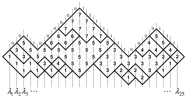
We now define the diagram of an interlacing sequence. See Figure 2. We start with a square grid; we denote the two directions defined by the grid lines with 0 and 1. A profile A=(A1,,AT1)𝐴subscript𝐴1subscript𝐴𝑇1A=(A_{1},\dots,A_{T-1}) is represented by a path of length T+1𝑇1T+1 on this grid where the path consists of grid edges whose directions are given by 0,A1,A2,,AT1,10subscript𝐴1subscript𝐴2subscript𝐴𝑇110,A_{1},A_{2},\dots,A_{T-1},1. This path forms the (upper) border of the diagram. Excluding the endpoints of the path we draw the diagonal rays (which form 45superscript4545^{\circ} angles with grid lines) starting at the vertices of the path and we index them (from left to right) with integers from 111 to T𝑇T. A diagram is a connected subset of boxes of a square grid whose (upper) border is given by the profile path and along the ithsuperscript𝑖𝑡i^{th} diagonal ray there are (λi)superscript𝜆𝑖\ell(\lambda^{i}) boxes. The filling numbers on the ithsuperscript𝑖𝑡i^{th} diagonal ray are parts of λisuperscript𝜆𝑖\lambda^{i} with the largest part at the top. Observe that by the definition of interlacing sequences we obtain monotone sequences of numbers in the direction of grid lines.

A (skew) plane partition and cylindric partition are examples of interlacing sequences. A plane partition can be written as Λ=(,λ1,,λT,)Λsuperscript𝜆1superscript𝜆𝑇\Lambda=(\emptyset,\lambda^{1},\dots,\lambda^{T},\emptyset) with profile A=(0,0,,0,1,,1,1)𝐴000111A=(0,0,\dots,0,1,\dots,1,1) and λisuperscript𝜆𝑖\lambda^{i}s are diagonals of the plane partition. A skew plane partition is an interlacing sequence Λ=(,λ1,,λT,)Λsuperscript𝜆1superscript𝜆𝑇\Lambda=(\emptyset,\lambda^{1},\dots,\lambda^{T},\emptyset) with a profile A=(0,A1,,AT1,1)𝐴0subscript𝐴1subscript𝐴𝑇11A=(0,A_{1},\dots,A_{T-1},1). A cylindric partition is an interlacing sequence Λ=(λ0,λ1,,λT)Λsuperscript𝜆0superscript𝜆1superscript𝜆𝑇\Lambda=(\lambda^{0},\lambda^{1},\dots,\lambda^{T}) where λ0=λTsuperscript𝜆0superscript𝜆𝑇\lambda^{0}=\lambda^{T}, and T𝑇T is called the period of ΛΛ\Lambda. A cylindric partition can be represented by the cylindric diagram that is obtained from the ordinary diagram by identification of the first and last diagonal.

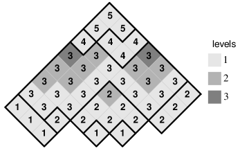
A connected component of an interlacing sequence ΛΛ\Lambda is the set of rookwise connected boxes of its diagram that are filled with a same number. We denote the number of connected components of ΛΛ\Lambda with k(Λ)𝑘Λk(\Lambda). For the example from Figure 2 we have k(Λ)=18𝑘Λ18k(\Lambda)=18 and its connected components are shown in Figure 2 (bold lines represent boundaries of these components).

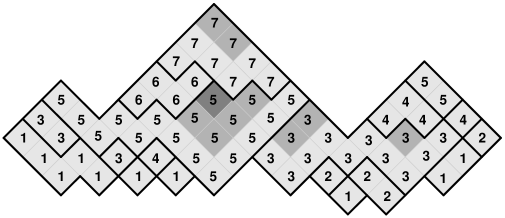
If a box (i,j)𝑖𝑗(i,j) belongs to a connected component C𝐶C then we define its level (i,j)𝑖𝑗\ell(i,j) as the smallest positive integer such that (i+,j+)𝑖𝑗(i+\ell,j+\ell) does not belong to C𝐶C. In other words, a level represents the distance from the “rim”, distance being measured diagonally. A border component is a rookwise connected subset of a connected component where all boxes have the same level. We also say that this border component is of this level. For the example from Figure 2, border components and their levels are shown in Figure 3 (different levels are represented by different colors).
Refer to caption
Figure 3. Border components with levels

Let (n1,n2,)subscript𝑛1subscript𝑛2(n_{1},n_{2},\dots) be a sequence of nonnegative integers where nisubscript𝑛𝑖n_{i} is the number of i𝑖i–level border components of ΛΛ\Lambda. We set

(1.8) AΛ(t)=i1(1ti)ni.subscript𝐴Λ𝑡subscriptproduct𝑖1superscript1superscript𝑡𝑖subscript𝑛𝑖A_{\Lambda}(t)=\prod_{i\geq 1}(1-t^{i})^{n_{i}}.

For the example above AΛ(t)=(1t)18(1t2)4(1t3)subscript𝐴Λ𝑡superscript1𝑡18superscript1superscript𝑡241superscript𝑡3A_{\Lambda}(t)=(1-t)^{18}(1-t^{2})^{4}(1-t^{3}).

For a cylindric partition ΠΠ\Pi, we define cylindric connected components and cylindric border components in the same way but connectedness is understood on the cylinder, i.e. boxes are connected if they are rookwise connected in the cylindric diagram. We define

AΠcyl(t)=i1(1ti)nicyl,superscriptsubscript𝐴Πcyl𝑡subscriptproduct𝑖1superscript1superscript𝑡𝑖subscriptsuperscript𝑛cyl𝑖A_{\Pi}^{\text{cyl}}(t)=\prod_{i\geq 1}(1-t^{i})^{n^{\text{cyl}}_{i}},

where nicylsubscriptsuperscript𝑛cyl𝑖n^{\text{cyl}}_{i} is the number of cylindric border components of level i𝑖i.

In Section 6 we give a generating function formula for skew plane partitions. Let Skew(T,A)Skew𝑇𝐴\text{Skew}(T,A) be the set of all skew plane partitions Λ=(,λ1,,λT,)Λsuperscript𝜆1superscript𝜆𝑇\Lambda=(\emptyset,\lambda^{1},\dots,\lambda^{T},\emptyset) with profile A=(A0,A1,,AT1,AT)𝐴subscript𝐴0subscript𝐴1subscript𝐴𝑇1subscript𝐴𝑇A=(A_{0},A_{1},\dots,A_{T-1},A_{T}), where A0=0subscript𝐴00A_{0}=0 and AT=1subscript𝐴𝑇1A_{T}=1.

Theorem 7.

(Generalized MacMahon’s formula for skew plane partitions; Hall-Littlewood case)

ΠSkew(T,A)AΠ(t)q|Π|=0i<jTAi=0,Aj=11tqji1qji.subscriptΠSkew𝑇𝐴subscript𝐴Π𝑡superscript𝑞Πsubscriptproduct0𝑖𝑗𝑇formulae-sequencesubscript𝐴𝑖0subscript𝐴𝑗11𝑡superscript𝑞𝑗𝑖1superscript𝑞𝑗𝑖\sum_{\Pi\in\text{Skew}(T,A)}A_{\Pi}(t)q^{|\Pi|}=\prod_{\begin{subarray}{c}0\leq i<j\leq T\\ A_{i}=0,\,A_{j}=1\end{subarray}}\frac{1-tq^{j-i}}{1-q^{j-i}}.

Note that as profiles are words in {0,1}01\{0,1\}, a profile A=(A0,,AT)𝐴subscript𝐴0subscript𝐴𝑇A=(A_{0},\dots,A_{T}) encodes the border of a Ferrers diagram λ𝜆\lambda. Skew plane partitions of profile A𝐴A are in one–to–one correspondence with reverse plane partitions of shape λ𝜆\lambda. Moreover, one can check that

0i<jTAi=0,Aj=11tqji1qji=(i,j)λ1tqhi,j1qhi,j.subscriptproduct0𝑖𝑗𝑇formulae-sequencesubscript𝐴𝑖0subscript𝐴𝑗11𝑡superscript𝑞𝑗𝑖1superscript𝑞𝑗𝑖subscriptproduct𝑖𝑗𝜆1𝑡superscript𝑞subscript𝑖𝑗1superscript𝑞subscript𝑖𝑗\prod_{\begin{subarray}{c}0\leq i<j\leq T\\ A_{i}=0,\,A_{j}=1\end{subarray}}\frac{1-tq^{j-i}}{1-q^{j-i}}=\prod_{(i,j)\in\lambda}\frac{1-tq^{h_{i,j}}}{1-q^{h_{i,j}}}.

Therefore the theorem of Gansner (equation (1.7)) is Theorem 7 with t=0𝑡0t=0 and our Theorem 5 on reverse plane overpartitions is Theorem 7 with t=1𝑡1t=-1.

This theorem is also a generalization of results of Vuletić [V2]. In [V2] a 2–parameter generalization of MacMahon’s formula related to Macdonald symmetric functions was given and the formula is especially simple in the Hall-Littlewood case. In the Hall-Littlewood case, this is a generating function formula for plane partitions weighted by AΠ(t)subscript𝐴Π𝑡A_{\Pi}(t). Theorem 7 can be naturally generalized to the Macdonald case, but we do not pursue this here.

Let Cyl(T,A)Cyl𝑇𝐴\text{Cyl}(T,A) be the set of all cylindric partitions with period T𝑇T and profile A=(A1,,AT)𝐴subscript𝐴1subscript𝐴𝑇A=(A_{1},\dots,A_{T}). The main result of Section 6 is:

Theorem 8.

(Generalized MacMahon’s formula for cylindric partitions; Hall-Littlewood case)

ΠCyl(T,A)AΠcyl(t)q|Π|=n=111qnT1i,jTAi=0,Aj=11tq(ji)(T)+(n1)T1q(ji)(T)+(n1)T,subscriptΠCyl𝑇𝐴subscriptsuperscript𝐴cylΠ𝑡superscript𝑞Πsuperscriptsubscriptproduct𝑛111superscript𝑞𝑛𝑇subscriptproductformulae-sequence1𝑖𝑗𝑇formulae-sequencesubscript𝐴𝑖0subscript𝐴𝑗11𝑡superscript𝑞subscript𝑗𝑖𝑇𝑛1𝑇1superscript𝑞subscript𝑗𝑖𝑇𝑛1𝑇\sum_{\Pi\in\text{Cyl}(T,A)}A^{\text{cyl}}_{\Pi}(t)q^{|\Pi|}=\prod_{n=1}^{\infty}\frac{1}{1-q^{nT}}\prod_{\begin{subarray}{c}1\leq i,j\leq T\\ A_{i}=0,\,A_{j}=1\end{subarray}}\frac{1-tq^{(j-i)_{(T)}+(n-1)T}}{1-q^{(j-i)_{(T)}+(n-1)T}},

where i(T)subscript𝑖𝑇i_{(T)} is the smallest positive integer such that ii(T) mod T𝑖subscript𝑖𝑇 mod 𝑇i\equiv i_{(T)}\text{ mod }T.

The case t=0𝑡0t=0 is due to Borodin and represents a generating function formula for cylindric partitions. Cylindric partitions were introduced and enumerated by Gessel and Krattenthaler [GK]. The result of Borodin could be also proven using Theorem 5 of [GK] and the SU(r)SU𝑟{\rm SU}(r)-extension of Bailey’s ψ66subscriptsubscript𝜓66{}_{6}\psi_{6} summation due to Gustafson (equation (7.9) in [GK]) [Kr3]. Again Theorem 8 can be naturally generalized to the Macdonald case. The trace generating function of those cylindric partitions could also be easily derived from our proof, as done by Okada [O] for the reverse plane partitions case.

The paper is organized as follows. In Section 2 we give a mostly combinatorial proof of the generalized MacMahon formula. In Section 3 we use nonintersecting paths and obtain the hook–length formulas for plane overpartitions and reverse plane partitions of a given shape. In Section 4 we make the connection between tilings and plane overpartitions. In Section 5 we construct a bijection between matrices and pairs of plane overpartitions and obtain a generating function formula for plane overpartitions with bounded part size. In Section 6 we give the hook formula for reverse plane partitions contained in a given shape and the 1–parameter generalization of the generating function formula for cylindric partitions. Section 7 contains some concluding remarks.

Acknowledgment. The authors want to thank Alexei Borodin, the advisor of the third author, for help and guidance and Cédric Boutillier, Dominique Gouyou-Beauchamps, Richard Kenyon and Jeremy Lovejoy for useful discussions. The authors also want to thank one of the anonymous referee for his long list of constructive comments.

2. Plane partitions and Hall–Littlewood functions

In this section, we give an alternative proof of the generalization of MacMahon’s formula due to the third author [V2]. Our proof is mostly combinatorial as it uses a bijection between plane partitions and pairs of strict plane partitions of the same shape and the combinatorial description of Hall–Littlewood functions ([Mac], Chapter III, Equation (5.11)).

Let 𝒫(r,c)𝒫𝑟𝑐{\mathcal{P}}(r,c) be the set of plane partitions with at most r𝑟r rows and c𝑐c columns. Given a plane partition ΠΠ\Pi, let AΠ(t)subscript𝐴Π𝑡A_{\Pi}(t) be the polynomial defined in (1.8), as AΠ(t)=rbordercomponent(1tlevel(r))subscript𝐴Π𝑡subscriptproduct𝑟bordercomponent1superscript𝑡level𝑟A_{\Pi}(t)=\prod_{r\ {\rm border}\ {\rm component}}(1-t^{{\rm level}(r)}).

Recall that Theorem 1.4 states that

Π𝒫(r,c)AΠ(t)q|Π|=i=1rj=1c1tqi+j11qi+j1.subscriptΠ𝒫𝑟𝑐subscript𝐴Π𝑡superscript𝑞Πsuperscriptsubscriptproduct𝑖1𝑟superscriptsubscriptproduct𝑗1𝑐1𝑡superscript𝑞𝑖𝑗11superscript𝑞𝑖𝑗1\sum_{\Pi\in{\mathcal{P}}(r,c)}A_{\Pi}(t)q^{|\Pi|}=\prod_{i=1}^{r}\prod_{j=1}^{c}\frac{1-tq^{i+j-1}}{1-q^{i+j-1}}.

Any plane partition ΠΠ\Pi is in bijection with a sequence of partitions (π(1),π(2),)superscript𝜋1superscript𝜋2(\pi^{(1)},\pi^{(2)},\ldots). This sequence is such that π(i)superscript𝜋𝑖\pi^{(i)} is the shape of the entries greater than or equal to i𝑖i in ΠΠ\Pi for all i𝑖i. For example if

Π=443333321,Π443333321\Pi=\begin{array}[]{l}4433\\ 3332\\ 1\end{array},

the corresponding sequence is ((4,4,1),(4,4),(4,3),(2))44144432((4,4,1),(4,4),(4,3),(2)).

Note that the plane partition ΠΠ\Pi is column strict if and only if π(i)/π(i+1)superscript𝜋𝑖superscript𝜋𝑖1\pi^{(i)}/\pi^{(i+1)} is a horizontal strip for all i𝑖i.

We use a bijection between pairs of column strict plane partitions (Σ,Λ)ΣΛ(\Sigma,\Lambda) and plane partitions ΠΠ\Pi due to Bender and Knuth [BK]. We suppose that (Σ,Λ)ΣΛ(\Sigma,\Lambda) are of the same shape λ𝜆\lambda and that the corresponding sequences are (σ(1),σ(2),)superscript𝜎1superscript𝜎2(\sigma^{(1)},\sigma^{(2)},\ldots) and (λ(1),λ(2),)superscript𝜆1superscript𝜆2(\lambda^{(1)},\lambda^{(2)},\ldots)

Given a plane partition Π=(Πi,j)ΠsubscriptΠ𝑖𝑗\Pi=(\Pi_{i,j}), we define the entries of diagonal x𝑥x to be the partition (Πi,j)subscriptΠ𝑖𝑗(\Pi_{i,j}) with i,j1𝑖𝑗1i,j\geq 1 and ji=x𝑗𝑖𝑥j-i=x. The bijection is such that the entries of diagonal x𝑥x of ΠΠ\Pi are σ(x+1)superscript𝜎𝑥1\sigma^{(x+1)} if x0𝑥0x\geq 0 and λ(x1)superscript𝜆𝑥1\lambda^{(-x-1)} otherwise. Note that as ΛΛ\Lambda and ΣΣ\Sigma have the same shape, the entries of the main diagonal (x=0𝑥0x=0) are σ(1)=λ(1)superscript𝜎1superscript𝜆1\sigma^{(1)}=\lambda^{(1)}.

For example, start with

Σ=44442221111 and Λ=44333322111,Σ44442221111 and Λ44333322111\Sigma=\begin{array}[]{l}4444\\ 2221\\ 111\end{array}\text{ and }\Lambda=\begin{array}[]{l}4433\\ 3322\\ 111\end{array},

whose sequences are ((4,4,3),(4,3),(4),(4))4434344((4,4,3),(4,3),(4),(4)) and ((4,4,3),(4,4),(4,2),(2))44344422((4,4,3),(4,4),(4,2),(2)), respectively and get

Π=444444344322.Π444444344322\Pi=\begin{array}[]{l}4444\\ 443\\ 443\\ 22\end{array}.

This construction implies that:

|Π|Π\displaystyle|\Pi| =\displaystyle= |Σ|+|Λ||λ|ΣΛ𝜆\displaystyle|\Sigma|+|\Lambda|-|\lambda|
AΠ(t)subscript𝐴Π𝑡\displaystyle A_{\Pi}(t) =\displaystyle= φΣ(t)φΛ(t)bλ(t).subscript𝜑Σ𝑡subscript𝜑Λ𝑡subscript𝑏𝜆𝑡\displaystyle\frac{\varphi_{\Sigma}(t)\varphi_{\Lambda}(t)}{b_{\lambda}(t)}.

Here we have

bλ(t)=i1φmi(λ)(t),φr(t)=j=1r(1tj),formulae-sequencesubscript𝑏𝜆𝑡subscriptproduct𝑖1subscript𝜑subscript𝑚𝑖𝜆𝑡subscript𝜑𝑟𝑡superscriptsubscriptproduct𝑗1𝑟1superscript𝑡𝑗b_{\lambda}(t)=\prod_{i\geq 1}\varphi_{m_{i}(\lambda)}(t),\ \ \ \varphi_{r}(t)=\prod_{j=1}^{r}(1-t^{j}),

and

φΛ(t)=i1φλ(i)/λ(i+1)(t).subscript𝜑Λ𝑡subscriptproduct𝑖1subscript𝜑superscript𝜆𝑖superscript𝜆𝑖1𝑡\varphi_{\Lambda}(t)=\prod_{i\geq 1}\varphi_{\lambda^{(i)}/\lambda^{(i+1)}}(t).

Moreover

φθ(t)=iI(1tmi(λ)),subscript𝜑𝜃𝑡subscriptproduct𝑖𝐼1superscript𝑡subscript𝑚𝑖𝜆\varphi_{\theta}(t)=\prod_{i\in I}(1-t^{m_{i}(\lambda)}),

where θ𝜃\theta is a horizontal strip λ/μ𝜆𝜇\lambda/\mu,mi(λ)subscript𝑚𝑖𝜆m_{i}(\lambda) is the multiplicity of i𝑖i in λ𝜆\lambda and I𝐼I is the set of integers such that θi=1subscriptsuperscript𝜃𝑖1\theta^{\prime}_{i}=1 and θi+1=0subscriptsuperscript𝜃𝑖10\theta^{\prime}_{i+1}=0. See [Mac], Chapter III Sections 2 and 5.

Indeed, the following statements are true.

  • Each factor (1ti)1superscript𝑡𝑖(1-t^{i}) in bλ(t)subscript𝑏𝜆𝑡b_{\lambda}(t) is in one-to-one correspondence with a border component of level i𝑖i that goes through the main diagonal of ΠΠ\Pi.

  • Each factor (1ti)1superscript𝑡𝑖(1-t^{i}) in φΣ(t)subscript𝜑Σ𝑡\varphi_{\Sigma}(t) is in one-to-one correspondence with a border component of level i𝑖i that ends in a non-negative diagonal.

  • Each factor (1ti)1superscript𝑡𝑖(1-t^{i}) in φΛ(t)subscript𝜑Λ𝑡\varphi_{\Lambda}(t) is in one-to-one correspondence with a border component of level i𝑖i that starts in a non-positive diagonal.

Continuing with our example, we have

φΣ(t)=(1t)2(1t2),φΛ(t)=(1t)3(1t2),bλ(t)=(1t)2(1t2),formulae-sequencesubscript𝜑Σ𝑡superscript1𝑡21superscript𝑡2formulae-sequencesubscript𝜑Λ𝑡superscript1𝑡31superscript𝑡2subscript𝑏𝜆𝑡superscript1𝑡21superscript𝑡2\varphi_{\Sigma}(t)=(1-t)^{2}(1-t^{2}),\ \ \ \varphi_{\Lambda}(t)=(1-t)^{3}(1-t^{2}),\ \ \ b_{\lambda}(t)=(1-t)^{2}(1-t^{2}),

and

AΠ(t)=(1t)3(1t2)=(1t)2(1t2)(1t)3(1t2)(1t)2(1t2).subscript𝐴Π𝑡superscript1𝑡31superscript𝑡2superscript1𝑡21superscript𝑡2superscript1𝑡31superscript𝑡2superscript1𝑡21superscript𝑡2A_{\Pi}(t)=(1-t)^{3}(1-t^{2})=\frac{(1-t)^{2}(1-t^{2})(1-t)^{3}(1-t^{2})}{(1-t)^{2}(1-t^{2})}.

We recall the combinatorial definition of the Hall–Littlewood functions following Macdonald [Mac]. The Hall-Littlewood function Qλ(x;t)subscript𝑄𝜆𝑥𝑡Q_{\lambda}(x;t) can be defined as

Qλ(x;t)=Λsh(Λ)=λφΛ(t)xΛ;subscript𝑄𝜆𝑥𝑡subscriptΛshΛ𝜆subscript𝜑Λ𝑡superscript𝑥ΛQ_{\lambda}(x;t)=\sum_{\begin{subarray}{c}\Lambda\\ {\rm sh}(\Lambda)=\lambda\end{subarray}}\varphi_{\Lambda}(t)x^{\Lambda};

where xΛ=x1α1x2α2superscript𝑥Λsuperscriptsubscript𝑥1subscript𝛼1superscriptsubscript𝑥2subscript𝛼2x^{\Lambda}=x_{1}^{\alpha_{1}}x_{2}^{\alpha_{2}}\ldots and αisubscript𝛼𝑖\alpha_{i} is the number of entries equal to i𝑖i in ΛΛ\Lambda. See [Mac] Chapter III, equation (5.11).

A direct consequence of the preceding bijection is that the entries of ΣΣ\Sigma are less than or equal to c𝑐c, and the entries of ΛΛ\Lambda are less than or equal to r𝑟r if and only if ΠΠ\Pi is in 𝒫(r,c)𝒫𝑟𝑐{\mathcal{P}}(r,c). Therefore :

Π𝒫(r,c)AΠ(t)q|Π|=λQλ(q,,qr,0,;t)Qλ(q0,,qc1,0,;t)bλ(t).subscriptΠ𝒫𝑟𝑐subscript𝐴Π𝑡superscript𝑞Πsubscript𝜆subscript𝑄𝜆𝑞superscript𝑞𝑟0𝑡subscript𝑄𝜆superscript𝑞0superscript𝑞𝑐10𝑡subscript𝑏𝜆𝑡\sum_{\Pi\in{\mathcal{P}}(r,c)}A_{\Pi}(t)q^{|\Pi|}=\sum_{\lambda}\frac{Q_{\lambda}(q,\ldots,q^{r},0,\ldots;t)Q_{\lambda}(q^{0},\ldots,q^{c-1},0,\ldots;t)}{b_{\lambda}(t)}.

Finally, we need equation (4.4) in Chapter III of [Mac].

(2.1) λQλ(x;t)Qλ(y;t)bλ(t)=i,j1txiyj1xiyj;subscript𝜆subscript𝑄𝜆𝑥𝑡subscript𝑄𝜆𝑦𝑡subscript𝑏𝜆𝑡subscriptproduct𝑖𝑗1𝑡subscript𝑥𝑖subscript𝑦𝑗1subscript𝑥𝑖subscript𝑦𝑗\sum_{\lambda}\frac{Q_{\lambda}(x;t)Q_{\lambda}(y;t)}{b_{\lambda}(t)}=\prod_{i,j}\frac{1-tx_{i}y_{j}}{1-x_{i}y_{j}};

With the substitutions xi=qisubscript𝑥𝑖superscript𝑞𝑖x_{i}=q^{i} for 1ir1𝑖𝑟1\leq i\leq r and 00 otherwise and yj=qj1subscript𝑦𝑗superscript𝑞𝑗1y_{j}=q^{j-1} for 1jc1𝑗𝑐1\leq j\leq c and 00 otherwise, we get the result.

3. Nonintersecting paths

3.1. Plane overpartitions of a given shape

In this section we represent plane overpartitions as nonintersecting paths. We use the determinantal formula for the number of nonintersecting paths (see [GV2, KM1, KM2, Li] ). Evaluating these determinants we obtain the hook–content formulas from Theorems 3 and 4. A similar approach was used for example in [Br] to compute super Schur functions.

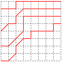
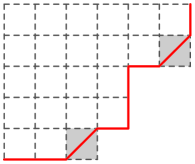
We construct a bijection between the set of paths from (0,0)00(0,0) to (x,k)𝑥𝑘(x,k) and the set of overpartitions with at most k𝑘k parts and the largest part at most x𝑥x. Given an overpartition the corresponding path consists of North and East edges that form the border of the Ferrers diagram of the overpartition except for corners containing an overlined entry where we substitute a pair of North and East edges with an North–East edge. For example, the path corresponding to the overpartition (6,6¯,4,4,3¯)6¯644¯3(6,\bar{6},4,4,\bar{3}) is shown in Figure 4. Note that this construction appears also in Proposition 2.2 of [Br].
Refer to caption
Figure 4. Paths and overpartitions

To each overpartition λ𝜆\lambda we associate a weight equal to ao(λ)q|λ|superscript𝑎𝑜𝜆superscript𝑞𝜆a^{o(\lambda)}q^{|\lambda|}, where o(λ)𝑜𝜆o(\lambda) is the number of overlined parts. To have the same weight on the corresponding path we introduce the following weights on edges. We assign weight 1 to East edges, qisuperscript𝑞𝑖q^{i} to North edges on (vertical) level i𝑖i and weight aqi+1𝑎superscript𝑞𝑖1aq^{i+1} to North-East edges joining vertical levels i𝑖i and i+1𝑖1i+1. The weight of the path is equal to the product of weights of its edges.

We will need the following lemma.

Lemma 1.

[CL] The generating function for overpartitions with at most k𝑘k parts is given by

(3.1) l(λ)kao(λ)q|λ|=(aq)k(q)ksubscript𝑙𝜆𝑘superscript𝑎𝑜𝜆superscript𝑞𝜆subscript𝑎𝑞𝑘subscript𝑞𝑘\sum_{l(\lambda)\leq k}{a^{o(\lambda)}q^{|\lambda|}}=\frac{(-aq)_{k}}{(q)_{k}}

and the generating function for overpartitions with exactly k𝑘k parts is given by

(3.2) l(λ)=kao(λ)q|λ|=qk(a)k(q)k.subscript𝑙𝜆𝑘superscript𝑎𝑜𝜆superscript𝑞𝜆superscript𝑞𝑘subscript𝑎𝑘subscript𝑞𝑘\sum_{l(\lambda)=k}{a^{o(\lambda)}q^{|\lambda|}}=q^{k}\frac{(-a)_{k}}{(q)_{k}}.

For a plane overpartition ΠΠ\Pi of shape λ𝜆\lambda we construct a set of nonintersecting paths using paths from row overpartitions where the starting point of the path corresponding to the i𝑖ith row is shifted upwards by λ1λi+i1subscript𝜆1subscript𝜆𝑖𝑖1\lambda_{1}-\lambda_{i}+i-1 so that the starting point is (0,λ1λi+i1)0subscript𝜆1subscript𝜆𝑖𝑖1(0,\lambda_{1}-\lambda_{i}+i-1). In that way, we obtain a bijection between the set of nonintersecting paths from (0,λ1λi+i1)0subscript𝜆1subscript𝜆𝑖𝑖1(0,\lambda_{1}-\lambda_{i}+i-1) to (x,λ1+i1),𝑥subscript𝜆1𝑖1(x,\lambda_{1}+i-1), where i𝑖i runs from 1 to (λ)𝜆\ell(\lambda), and the set of plane overpartitions whose i𝑖ith row has at most λisubscript𝜆𝑖\lambda_{i} parts and at least λi1subscript𝜆𝑖1\lambda_{i-1} parts with x𝑥x greater or equal to the largest part. The weights of this set of nonintersecting paths (the product of weights of its paths) is equal to ao(Π)q|Π|superscript𝑎𝑜Πsuperscript𝑞Πa^{o(\Pi)}q^{|\Pi|}. Figure 5 (see also Figure 8) shows the corresponding set of nonintersecting paths for x=8𝑥8x=8 and the plane overpartition

743¯22¯333¯2¯3¯21¯2.74¯32¯233¯3¯2missing-subexpression¯32¯1missing-subexpressionmissing-subexpression2missing-subexpressionmissing-subexpressionmissing-subexpressionmissing-subexpression\begin{array}[]{lllll}7&4&\bar{3}&2&\bar{2}\\ 3&3&\bar{3}&\bar{2}\\ \bar{3}&2&\bar{1}&&\\ 2&&&&\end{array}.
Refer to caption
Figure 5. Nonintersecting paths
Definition 1.

For a partition λ𝜆\lambda we define Mλ(a;q)subscript𝑀𝜆𝑎𝑞M_{\lambda}(a;q) to be the (λ)×(λ)𝜆𝜆\ell(\lambda)\times\ell(\lambda) matrix whose (i,j)𝑖𝑗(i,j)th entry is given by

(a)λj+ij(q)λj+ij.subscript𝑎subscript𝜆𝑗𝑖𝑗subscript𝑞subscript𝜆𝑗𝑖𝑗\frac{(-a)_{\lambda_{j}+i-j}}{(q)_{\lambda_{j}+i-j}}.

For a partition λ𝜆\lambda let (λ)𝜆\mathcal{B}(\lambda) and 𝒮(λ)𝒮𝜆\mathcal{S}(\lambda) be as in the introduction, i.e. the sets of all plane overpartitions bounded by shape λ𝜆\lambda and of the shape λ𝜆\lambda, respectively.

Proposition 1.

Let λ𝜆\lambda be a partition. The weighted generating function for plane overpartitions whose ithsuperscript𝑖𝑡i^{th} row is an overpartition that has at most λisubscript𝜆𝑖\lambda_{i} parts and at least λi+1subscript𝜆𝑖1\lambda_{i+1} parts is given by

Π(λ)ao(Π)q|Π|=detMλ(aq;q).subscriptΠ𝜆superscript𝑎𝑜Πsuperscript𝑞Πsubscript𝑀𝜆𝑎𝑞𝑞\sum_{\Pi\in\mathcal{B}(\lambda)}a^{o(\Pi)}q^{|\Pi|}=\det M_{\lambda}(aq;q).
Proof.

From (3.1) we have that the limit when x𝑥x runs to infinity of the number of paths from (0,0)00(0,0) to (x,k)𝑥𝑘(x,k) is (aq)k/(q)ksubscript𝑎𝑞𝑘subscript𝑞𝑘(-aq)_{k}/(q)_{k}. Using Lemma 1 of [Li] we have that detMλ(aq;q)subscript𝑀𝜆𝑎𝑞𝑞\det M_{\lambda}(aq;q) is the limit when x𝑥x goes to infinity of the generating function for (λ)𝜆\ell(\lambda) nonintersecting paths going from (0,λ1+i1λi)0subscript𝜆1𝑖1subscript𝜆𝑖(0,\lambda_{1}+i-1-\lambda_{i}) to (x,λ1+i1)𝑥subscript𝜆1𝑖1(x,\lambda_{1}+i-1). Thanks to the bijection between paths and overpartitions this is also the generating function for overpartitions whose i𝑖ith row overpartition has at most λisubscript𝜆𝑖\lambda_{i} and at least λi+1subscript𝜆𝑖1\lambda_{i+1} parts. ∎

Proposition 2.

Let λ𝜆\lambda be a partition. The weighted generating function for plane overpartitions of shape λ𝜆\lambda is given by

Π𝒮(λ)ao(Π)q|Π|=q|λ|detMλ(a;q).subscriptΠ𝒮𝜆superscript𝑎𝑜Πsuperscript𝑞Πsuperscript𝑞𝜆subscript𝑀𝜆𝑎𝑞\sum_{\Pi\in\mathcal{S}(\lambda)}a^{o(\Pi)}q^{|\Pi|}=q^{|\lambda|}\det M_{\lambda}(a;q).
Proof.

The proof is the same as the proof of Proposition 1. Here we just use (3.2) instead of (3.1). ∎

The determinant of Mλ(a;q)subscript𝑀𝜆𝑎𝑞M_{\lambda}(a;q) is given by the following formula:

(3.3) detMλ(a;q)=qi(i1)λi(i,j)λ1+aqci,j1qhi,j.subscript𝑀𝜆𝑎𝑞superscript𝑞subscript𝑖𝑖1subscript𝜆𝑖subscriptproduct𝑖𝑗𝜆1𝑎superscript𝑞subscript𝑐𝑖𝑗1superscript𝑞subscript𝑖𝑗\det M_{\lambda}(a;q)=q^{\sum_{i}(i-1)\lambda_{i}}\prod_{(i,j)\in\lambda}\frac{1+aq^{c_{i,j}}}{1-q^{h_{i,j}}}.

For the proof see for example pages 16–17 of [GV2] or Theorem 26 (3.11) of [Kr2].

Using (3.3) we obtain the product formulas for the generating functions from Propositions 1 and 2. Those are the hook–content formulas given in Theorems 3 and 4.

Remark 1. We give a bijective proof of formula (3.3). Indeed Krattenthaler [Kr1] showed that the weighted generating function of super semistandard Young tableaux of shape λ𝜆\lambda is

qi(i1)λi(i,j)λ1+aqci,j1qhi,j,superscript𝑞subscript𝑖𝑖1subscript𝜆𝑖subscriptproduct𝑖𝑗𝜆1𝑎superscript𝑞subscript𝑐𝑖𝑗1superscript𝑞subscript𝑖𝑗q^{\sum_{i}(i-1)\lambda_{i}}\prod_{(i,j)\in\lambda}\frac{1+aq^{c_{i,j}}}{1-q^{h_{i,j}}},

where each tableau is weighted by ao(T)q|T|superscript𝑎𝑜𝑇superscript𝑞𝑇a^{o(T)}q^{|T|}. A super semistandard tableau [Kr1] of shape λ𝜆\lambda is a filling of cells of the Ferrers diagram of λ𝜆\lambda with entries from the ordered alphabet 1<2<3<<1¯<2¯<3¯<123¯1¯2¯31<2<3<\ldots<\bar{1}<\bar{2}<\bar{3}<\ldots such that

  • the nonoverlined entries form a column-strict reverse plane partition of some shape ν𝜈\nu, where ν𝜈\nu is a partition contained in λ𝜆\lambda,

  • the overlined entries form a row-strict reverse plane partition of shape λ/ν𝜆𝜈\lambda/\nu.

We give here a bijection from super semistandard Young tableaux to plane overpartitions. We starting with a super semistandard Young tableau where the nonoverlined (resp. overlined) entries are less than or equal to k𝑘k (resp. \ell). First, change all the entries equal to a𝑎a by k+1a𝑘1𝑎k+1-a and all the entries equal to a¯¯𝑎\bar{a} to +1a¯¯1𝑎\overline{\ell+1-a}.

For example, starting with the super semistandard Young tableau with k=5𝑘5k=5 and =44\ell=4

134552¯4¯2451¯2¯3¯4¯352¯3¯4¯41¯3¯3¯we obtain532113¯1¯4214¯3¯2¯1¯313¯2¯1¯24¯2¯2¯.13455¯2¯4245¯1¯2¯3¯435¯2¯3¯44¯1¯3¯3we obtain53211¯3¯1421¯4¯3¯2¯131¯3¯2¯12¯4¯2¯2\begin{array}[]{l}13455\bar{2}\bar{4}\\ 245\bar{1}\bar{2}\bar{3}\bar{4}\\ 35\bar{2}\bar{3}\bar{4}\\ 4\bar{1}\bar{3}\\ \bar{3}\end{array}\quad\textrm{we obtain}\quad\begin{array}[]{l}53211\bar{3}\bar{1}\\ 421\bar{4}\bar{3}\bar{2}\bar{1}\\ 31\bar{3}\bar{2}\bar{1}\\ 2\bar{4}\bar{2}\\ \bar{2}\end{array}.

Now we use the order 0<1¯<1<2¯<2<3¯<3<0¯11¯22¯330<\bar{1}<1<\bar{2}<2<\bar{3}<3<\ldots and we suppose that the cells outside of the shape λ𝜆\lambda are filled with 0. At first all the nonoverlined entries are active. While there is an active part, we choose the smallest active part. If there are more than one, we choose the rightmost one. We swap it with its east or south neighbor, choosing the larger of the two. If they are equal then we choose the east one. We proceed in this way until this part is greater than or equal to both of its neighbors. When we reach this, we declare the part inactive.

Continuing with the preceding example and applying the algorithm to the smallest (and rightmost) active part until it becomes inactive we obtain:

𝟓𝟑𝟐𝟏𝟏3¯1¯𝟒𝟐𝟏4¯3¯2¯1¯𝟑𝟏3¯2¯1¯𝟐4¯2¯2¯𝟓𝟑𝟐𝟏3¯𝟏1¯𝟒𝟐𝟏4¯3¯2¯1¯𝟑𝟏3¯2¯1¯𝟐4¯2¯2¯𝟓𝟑𝟐𝟏3¯2¯1¯𝟒𝟐𝟏4¯3¯𝟏1¯𝟑𝟏3¯2¯1¯𝟐4¯2¯2¯53211¯3¯1421¯4¯3¯2¯131¯3¯2¯12¯4¯2¯25321¯31¯1421¯4¯3¯2¯131¯3¯2¯12¯4¯2¯25321¯3¯2¯1421¯4¯31¯131¯3¯2¯12¯4¯2¯2\begin{array}[]{l}{\bf 5321}{\bf 1}\bar{3}\bar{1}\\ {\bf 421}\bar{4}\bar{3}\bar{2}\bar{1}\\ {\bf 31}\bar{3}\bar{2}\bar{1}\\ {\bf 2}\bar{4}\bar{2}\\ \bar{2}\end{array}\ \ \ \begin{array}[]{l}{\bf 5321}\bar{3}{\bf 1}\bar{1}\\ {\bf 421}\bar{4}\bar{3}\bar{2}\bar{1}\\ {\bf 31}\bar{3}\bar{2}\bar{1}\\ {\bf 2}\bar{4}\bar{2}\\ \bar{2}\end{array}\ \ \ \begin{array}[]{l}{\bf 5321}\bar{3}\bar{2}\bar{1}\\ {\bf 421}\bar{4}\bar{3}{\bf 1}\bar{1}\\ {\bf 31}\bar{3}\bar{2}\bar{1}\\ {\bf 2}\bar{4}\bar{2}\\ \bar{2}\end{array}

Then we move the rest of the active parts.

𝟓𝟑𝟐4¯3¯2¯1¯𝟒𝟐𝟏3¯111¯𝟑𝟏3¯2¯1¯𝟐4¯2¯2¯𝟓𝟑𝟐4¯3¯2¯1¯𝟒𝟐3¯2¯111¯𝟑𝟏3¯11¯𝟐4¯2¯2¯𝟓𝟑𝟐4¯3¯2¯1¯𝟒𝟐3¯2¯111¯𝟑4¯3¯11¯𝟐2¯𝟏2¯𝟓𝟑𝟐4¯3¯2¯1¯𝟒𝟐3¯2¯111¯𝟑4¯3¯11¯𝟐2¯12¯𝟓𝟑4¯3¯22¯1¯𝟒𝟐3¯2¯111¯𝟑4¯3¯11¯𝟐2¯12¯532¯4¯3¯2¯1421¯311¯131¯3¯2¯12¯4¯2¯2532¯4¯3¯2¯142¯3¯211¯131¯31¯12¯4¯2¯2532¯4¯3¯2¯142¯3¯211¯13¯4¯31¯12¯21¯2532¯4¯3¯2¯142¯3¯211¯13¯4¯31¯12¯21¯253¯4¯32¯2¯142¯3¯211¯13¯4¯31¯12¯21¯2\begin{array}[]{l}{\bf 532}\bar{4}\bar{3}\bar{2}\bar{1}\\ {\bf 421}\bar{3}1{1}\bar{1}\\ {\bf 31}\bar{3}\bar{2}\bar{1}\\ {\bf 2}\bar{4}\bar{2}\\ \bar{2}\end{array}\ \ \ \begin{array}[]{l}{\bf 532}\bar{4}\bar{3}\bar{2}\bar{1}\\ {\bf 42}\bar{3}\bar{2}11\bar{1}\\ {\bf 31}\bar{3}{1}\bar{1}\\ {\bf 2}\bar{4}\bar{2}\\ \bar{2}\end{array}\ \ \ \begin{array}[]{l}{\bf 532}\bar{4}\bar{3}\bar{2}\bar{1}\\ {\bf 42}\bar{3}\bar{2}11\bar{1}\\ {\bf 3}\bar{4}\bar{3}{1}\bar{1}\\ {\bf 2}\bar{2}{\bf 1}\\ \bar{2}\end{array}\ \ \ \begin{array}[]{l}{\bf 532}\bar{4}\bar{3}\bar{2}\bar{1}\\ {\bf 42}\bar{3}\bar{2}11\bar{1}\\ {\bf 3}\bar{4}\bar{3}{1}\bar{1}\\ {\bf 2}\bar{2}{1}\\ \bar{2}\end{array}\ \ \ \begin{array}[]{l}{\bf 53}\bar{4}\bar{3}2\bar{2}\bar{1}\\ {\bf 42}\bar{3}\bar{2}11\bar{1}\\ {\bf 3}\bar{4}\bar{3}{1}\bar{1}\\ {\bf 2}\bar{2}{1}\\ \bar{2}\end{array}
𝟓𝟑4¯3¯22¯1¯𝟒4¯3¯2¯111¯𝟑3¯211¯𝟐2¯12¯𝟓𝟑4¯3¯22¯1¯𝟒4¯3¯2¯111¯𝟑3¯211¯2¯212¯𝟓4¯33¯22¯1¯𝟒4¯3¯2¯111¯𝟑3¯211¯2¯212¯𝟓4¯33¯22¯1¯𝟒4¯3¯2¯111¯33¯211¯2¯212¯𝟓4¯33¯22¯1¯44¯3¯2¯111¯33¯211¯2¯212¯53¯4¯32¯2¯14¯4¯3¯211¯13¯321¯12¯21¯253¯4¯32¯2¯14¯4¯3¯211¯13¯321¯1¯221¯25¯43¯32¯2¯14¯4¯3¯211¯13¯321¯1¯221¯25¯43¯32¯2¯14¯4¯3¯211¯13¯321¯1¯221¯25¯43¯32¯2¯14¯4¯3¯211¯13¯321¯1¯221¯2\begin{array}[]{l}{\bf 53}\bar{4}\bar{3}2\bar{2}\bar{1}\\ {\bf 4}\bar{4}\bar{3}\bar{2}11\bar{1}\\ {\bf 3}\bar{3}2{1}\bar{1}\\ {\bf 2}\bar{2}{1}\\ \bar{2}\end{array}\ \ \ \begin{array}[]{l}{\bf 53}\bar{4}\bar{3}2\bar{2}\bar{1}\\ {\bf 4}\bar{4}\bar{3}\bar{2}11\bar{1}\\ {\bf 3}\bar{3}2{1}\bar{1}\\ \bar{2}2{1}\\ \bar{2}\end{array}\ \ \ \begin{array}[]{l}{\bf 5}\bar{4}3\bar{3}2\bar{2}\bar{1}\\ {\bf 4}\bar{4}\bar{3}\bar{2}11\bar{1}\\ {\bf 3}\bar{3}2{1}\bar{1}\\ \bar{2}2{1}\\ \bar{2}\end{array}\ \ \ \begin{array}[]{l}{\bf 5}\bar{4}3\bar{3}2\bar{2}\bar{1}\\ {\bf 4}\bar{4}\bar{3}\bar{2}11\bar{1}\\ {3}\bar{3}2{1}\bar{1}\\ \bar{2}2{1}\\ \bar{2}\end{array}\ \ \ \begin{array}[]{l}{\bf 5}\bar{4}3\bar{3}2\bar{2}\bar{1}\\ {4}\bar{4}\bar{3}\bar{2}11\bar{1}\\ {3}\bar{3}2{1}\bar{1}\\ \bar{2}2{1}\\ \bar{2}\end{array}

Remark 2. Stanley’s hook–content formula states that the generating function of semistandard Young tableaux of shape λ𝜆\lambda where the entries are less than or equal to n𝑛n is

(3.4) q(i1)λi(i,j)λ1qn+ci,j1qhi,j.superscript𝑞𝑖1subscript𝜆𝑖subscriptproduct𝑖𝑗𝜆1superscript𝑞𝑛subscript𝑐𝑖𝑗1superscript𝑞subscript𝑖𝑗q^{\sum(i-1)\lambda_{i}}\prod_{(i,j)\in\lambda}\frac{1-q^{n+c_{i,j}}}{1-q^{h_{i,j}}}.

See Theorem 7.21.2 of [Sta]. Formula (3.3) is equivalent to Stanley’s hook formula by Examples I.2.5 and I.3.3 of [Mac]. Again we can give a bijective argument.

Formula (3.4) is the weighted generating function of super semistandard tableaux of shape λ𝜆\lambda with a=qn𝑎superscript𝑞𝑛a=-q^{n}. Start with a super semistandard Young tableau T𝑇T of shape λ𝜆\lambda and add n𝑛n to all the overlined entries. Now transform the tableau into a reverse plane overpartition with the above algorithm using the order 1>1¯>2>2¯>3>1¯12¯231>\bar{1}>2>\bar{2}>3>\ldots. This shows that super semistandard Young tableaux T𝑇T of shape λ𝜆\lambda with weight (qn)o(T)q|T|superscriptsuperscript𝑞𝑛𝑜𝑇superscript𝑞𝑇(-q^{n})^{o(T)}q^{|T|} are in bijection with reverse plane overpartitions ΠΠ\Pi of the same shape where the overlined entries are greater than n𝑛n with weight (1)o(Π)q|Π|superscript1𝑜Πsuperscript𝑞Π(-1)^{o(\Pi)}q^{|\Pi|}.

Now we define a sign reversing involution on these reverse plane overpartitions. Given such a reverse plane overpartition, if there is at least one part greater than n𝑛n, we choose the uppermost and rightmost part greater than n𝑛n. If this part is overlined, then we take off the overline, otherwise we overline the part. Note that in this case the parity of the number of overlined parts is changed and therefore the weight of the reverse plane overpartition is multiplied by 11-1. If no such part exists, the given reverse plane partition is a semistandard Young tableau of shape λ𝜆\lambda where the entries are less than or equal to n𝑛n.

Now, we give a generating formula for plane overpartitions with at most r𝑟r rows and c𝑐c columns.

Proposition 3.

The weighted generating function for plane overpartitions with at most r𝑟r rows and c𝑐c columns is given by

cλ1λ(r1)/20detM(c,λ1,λ1,,λ(r1)/2,λ(r1)/2)(aq;q)subscript𝑐subscript𝜆1subscript𝜆𝑟120subscript𝑀𝑐subscript𝜆1subscript𝜆1subscript𝜆𝑟12subscript𝜆𝑟12𝑎𝑞𝑞\sum_{c\geq\lambda_{1}\geq\ldots\geq\lambda_{(r-1)/2}\geq 0}\det M_{(c,\lambda_{1},\lambda_{1},\ldots,\lambda_{(r-1)/2},\lambda_{(r-1)/2})}(aq;q)

if r𝑟r is odd, and by

cλ1λr/20detM(λ1,λ1,,λr/2,λr/2)(aq;q)subscript𝑐subscript𝜆1subscript𝜆𝑟20subscript𝑀subscript𝜆1subscript𝜆1subscript𝜆𝑟2subscript𝜆𝑟2𝑎𝑞𝑞\sum_{c\geq\lambda_{1}\geq\ldots\geq\lambda_{r/2}\geq 0}\det M_{(\lambda_{1},\lambda_{1},\ldots,\lambda_{r/2},\lambda_{r/2})}(aq;q)

if r𝑟r is even.

In particular, the weighted generating function for all overpartitions is:

λ1λkdetM(λ1,λ1,,λk,λk)(aq;q).subscriptsubscript𝜆1subscript𝜆𝑘subscript𝑀subscript𝜆1subscript𝜆1subscript𝜆𝑘subscript𝜆𝑘𝑎𝑞𝑞\sum_{\lambda_{1}\geq\ldots\geq\lambda_{k}}\det M_{(\lambda_{1},\lambda_{1},\ldots,\lambda_{k},\lambda_{k})}(aq;q).
Proof.

This is a direct consequence of Proposition 1. ∎

We will use this result to get another “symmetric function” proof of the shifted MacMahon’s formula ([FW1, V1, V2]):

Π is a planeoverpartitionq|Π|=n=1(1+qn1qn)n.subscriptΠ is a planeoverpartitionsuperscript𝑞Πsuperscriptsubscriptproduct𝑛1superscript1superscript𝑞𝑛1superscript𝑞𝑛𝑛\sum_{\begin{subarray}{c}\Pi\text{ is a plane}\\ \text{overpartition}\end{subarray}}q^{|\Pi|}=\prod_{n=1}^{\infty}\left(\frac{1+q^{n}}{1-q^{n}}\right)^{n}.

3.2. The weighted shifted MacMahon formula

In this section we give the weighted generalization of the shifted MacMahon formula. We use a symmetric function identity to compute the last sum in Proposition 3 since detMλ(a;q)subscript𝑀𝜆𝑎𝑞\det M_{\lambda}(a;q), as we will soon see, has an interpretation in terms of symmetric functions.

A symmetric function of an alphabet (set of indeterminates, also called letters) 𝔸𝔸\mathbb{A} is a function of letters which is invariant under any permutation of 𝔸𝔸\mathbb{A}. Recall three standard bases for the algebra of symmetric functions: Schur functions s𝑠s, complete symmetric functions hh and elementary symmetric functions e𝑒e (see [Mac]). The latter two are conveniently given by their generating functions:

Ht(𝔸)=aA11taandEt(𝔸)=aA(1+ta).formulae-sequencesubscript𝐻𝑡𝔸subscriptproduct𝑎𝐴11𝑡𝑎andsubscript𝐸𝑡𝔸subscriptproduct𝑎𝐴1𝑡𝑎H_{t}(\mathbb{A})=\prod_{a\in A}\frac{1}{1-ta}\quad\text{and}\quad E_{t}(\mathbb{A})=\prod_{a\in A}(1+ta).

Algebraic operations on alphabets, such as addition, subtraction and multiplication, can be defined using λ𝜆\lambda-rings framework, see Chapters I and II of [La]. In this framework symmetric functions are seen as ring operators. The addition of two alphabets 𝔸𝔸\mathbb{A} and 𝔹𝔹\mathbb{B} is defined naturally as their disjoint union and is denoted by 𝔸+𝔹𝔸𝔹\mathbb{A}+\mathbb{B}. Obviously,

Ht(𝔸+𝔹)=Ht(𝔸)Ht(𝔹).subscript𝐻𝑡𝔸𝔹subscript𝐻𝑡𝔸subscript𝐻𝑡𝔹H_{t}(\mathbb{A}+\mathbb{B})=H_{t}(\mathbb{A})H_{t}(\mathbb{B}).

Subtraction and multiplication are defined by

Ht(𝔸𝔹)=Ht(𝔸)Ht(𝔹),Ht(c𝔸)=(Ht(𝔸))c,c.formulae-sequencesubscript𝐻𝑡𝔸𝔹subscript𝐻𝑡𝔸subscript𝐻𝑡𝔹formulae-sequencesubscript𝐻𝑡𝑐𝔸superscriptsubscript𝐻𝑡𝔸𝑐𝑐H_{t}(\mathbb{A}-\mathbb{B})=\frac{H_{t}(\mathbb{A})}{H_{t}(\mathbb{B})},\quad\quad H_{t}(c\mathbb{A})=(H_{t}(\mathbb{A}))^{c},\quad c\in\mathbb{C}.

Analogous relations hold for elementary symmetric functions since Et(𝔸)=Ht(𝔸)subscript𝐸𝑡𝔸subscript𝐻𝑡𝔸E_{t}(\mathbb{A})=H_{-t}(-\mathbb{A}).

A specialization is an algebra homomorphism between the algebra of symmetric functions and \mathbb{C}. If ρ𝜌\rho is a specialization and f𝑓f is a symmetric function we denote its image by f|ρevaluated-at𝑓𝜌f|_{\rho}.

Let ρ(a)𝜌𝑎\rho(a) be a specialization given by

hn|ρ(a)=(a)n(q)n.evaluated-atsubscript𝑛𝜌𝑎subscript𝑎𝑛subscript𝑞𝑛h_{n}|_{\rho(a)}=\frac{(-a)_{n}}{(q)_{n}}.

Since, for λ=(λ1,λ2,,λk)𝜆subscript𝜆1subscript𝜆2subscript𝜆𝑘\lambda={(\lambda_{1},\lambda_{2},\dots,\lambda_{k})}

sλ=det(hλii+j)subscript𝑠𝜆subscriptsubscript𝜆𝑖𝑖𝑗s_{\lambda}=\det(h_{\lambda_{i}-i+j})

we have from Definition 1 that

(3.5) sλ|ρ(a)=detMλ(a;q).evaluated-atsubscript𝑠𝜆𝜌𝑎subscript𝑀𝜆𝑎𝑞s_{\lambda}|_{\rho(a)}=\det M_{\lambda}(a;q).

In the λ𝜆\lambda–ring framework, the q𝑞q-binomial theorem (see (2.21) of [A])

n=0(a)n(q)ntn=(at)(t)superscriptsubscript𝑛0subscript𝑎𝑛subscript𝑞𝑛superscript𝑡𝑛subscript𝑎𝑡subscript𝑡\sum_{n=0}^{\infty}\frac{(-a)_{n}}{(q)_{n}}t^{n}=\frac{(-at)_{\infty}}{(t)_{\infty}}

shows that the specialization ρ(a)𝜌𝑎\rho(a) is equivalent to considering symmetric functions in the difference of two alphabets 1+q+q2+1𝑞superscript𝑞21+q+q^{2}+\cdots and aaqaq2𝑎𝑎𝑞𝑎superscript𝑞2-a-aq-aq^{2}-\cdots. Thus,

sλ|ρ(a)=sλ((1+q+q2+)(aaqaq2aq3)).evaluated-atsubscript𝑠𝜆𝜌𝑎subscript𝑠𝜆1𝑞superscript𝑞2𝑎𝑎𝑞𝑎superscript𝑞2𝑎superscript𝑞3s_{\lambda}|_{\rho(a)}=s_{\lambda}((1+q+q^{2}+\cdots)-(-a-aq-aq^{2}-aq^{3}-\cdots)).

The weighted shifted MacMahon formula can be obtained from (3.5) and Proposition 3. We have

Π is a planeoverpartitionao(π)q|Π|=λ1λ2λks(λ1,λ1,λ2,λ2,,λk,λk)|ρ(aq)=λ evensλ|ρ(aq),subscriptΠ is a planeoverpartitionsuperscript𝑎𝑜𝜋superscript𝑞Πevaluated-atsubscriptsubscript𝜆1subscript𝜆2subscript𝜆𝑘subscript𝑠subscript𝜆1subscript𝜆1subscript𝜆2subscript𝜆2subscript𝜆𝑘subscript𝜆𝑘𝜌𝑎𝑞evaluated-atsubscriptsuperscript𝜆 evensubscript𝑠𝜆𝜌𝑎𝑞\sum_{\begin{subarray}{c}\Pi\text{ is a plane}\\ \text{overpartition}\end{subarray}}a^{o(\pi)}q^{|\Pi|}=\sum_{\lambda_{1}\geq\lambda_{2}\geq\cdots\geq\lambda_{k}}s_{(\lambda_{1},\lambda_{1},\lambda_{2},\lambda_{2},\dots,\lambda_{k},\lambda_{k})}|_{\rho(aq)}=\sum_{\lambda^{\prime}\text{ even}}s_{\lambda}|_{\rho(aq)},

where λsuperscript𝜆\lambda^{\prime} is the transpose of λ𝜆\lambda and a partition is even if it has even parts.

By Ex. 10 b) on p. 79 of [Mac] we have

λ evensλ(𝔸)t|λ|/2=Ht(e2(𝔸)).subscriptsuperscript𝜆 evensubscript𝑠𝜆𝔸superscript𝑡𝜆2subscript𝐻𝑡subscript𝑒2𝔸\sum_{\lambda^{\prime}\text{ even}}s_{\lambda}(\mathbb{A})t^{|\lambda|/2}=H_{t}(e_{2}(\mathbb{A})).

If instead of 𝔸𝔸\mathbb{A} we insert a difference of alphabets 𝔸=x1+x2+𝔸subscript𝑥1subscript𝑥2\mathbb{A}=x_{1}+x_{2}+\dots and 𝔹=y1+y2+𝔹subscript𝑦1subscript𝑦2\mathbb{B}=y_{1}+y_{2}+\dots then we obtain the following product formula:

λ evensλ(𝔸𝔹)t|λ|/2subscriptsuperscript𝜆 evensubscript𝑠𝜆𝔸𝔹superscript𝑡𝜆2\displaystyle\sum_{\lambda^{\prime}\text{ even}}s_{\lambda}(\mathbb{A}-\mathbb{B})t^{|\lambda|/2} =\displaystyle= Ht(e2(𝔸𝔹))subscript𝐻𝑡subscript𝑒2𝔸𝔹\displaystyle H_{t}(e_{2}(\mathbb{A}-\mathbb{B}))
=\displaystyle= Ht(1i<jxixj+1ijyiyj1i,jxiyj)subscript𝐻𝑡subscript1𝑖𝑗subscript𝑥𝑖subscript𝑥𝑗subscript1𝑖𝑗subscript𝑦𝑖subscript𝑦𝑗subscript1𝑖𝑗subscript𝑥𝑖subscript𝑦𝑗\displaystyle H_{t}\Big{(}\sum_{1\leq i<j}x_{i}x_{j}+\sum_{1\leq i\leq j}y_{i}y_{j}-\sum_{1\leq i,j}x_{i}y_{j}\Big{)}
=\displaystyle= 1i<j11xixjt1ij11yiyjt1i,j(1xiyjt).subscriptproduct1𝑖𝑗11subscript𝑥𝑖subscript𝑥𝑗𝑡subscriptproduct1𝑖𝑗11subscript𝑦𝑖subscript𝑦𝑗𝑡subscriptproduct1𝑖𝑗1subscript𝑥𝑖subscript𝑦𝑗𝑡\displaystyle\prod_{1\leq i<j}\frac{1}{1-x_{i}x_{j}t}\prod_{1\leq i\leq j}\frac{1}{1-y_{i}y_{j}t}\prod_{1\leq i,j}(1-x_{i}y_{j}t).

This gives us the weighted shifted MacMahon formula:

Proposition 4.

The weighted generating formula for plane overpartitions is

Π is a planeoverpartitionao(Π)q|Π|=i=1(1+aqi)i(1qi)i/2(1a2qi)i/2.subscriptΠ is a planeoverpartitionsuperscript𝑎𝑜Πsuperscript𝑞Πsuperscriptsubscriptproduct𝑖1superscript1𝑎superscript𝑞𝑖𝑖superscript1superscript𝑞𝑖𝑖2superscript1superscript𝑎2superscript𝑞𝑖𝑖2\sum_{\begin{subarray}{c}\Pi\text{ is a plane}\\ \text{overpartition}\end{subarray}}a^{o(\Pi)}q^{|\Pi|}=\prod_{i=1}^{\infty}\frac{(1+aq^{i})^{i}}{(1-q^{i})^{\lceil i/2\rceil}(1-a^{2}q^{i})^{\lfloor i/2\rfloor}}.
Proof.

Substituting xi=qi1subscript𝑥𝑖superscript𝑞𝑖1x_{i}=q^{i-1} and yi=aqisubscript𝑦𝑖𝑎superscript𝑞𝑖y_{i}=-aq^{i} in the preceding product formula, we get

0i<j11qi+j1ij11a2qi+j1i,j(1+aqi+j1).subscriptproduct0𝑖𝑗11superscript𝑞𝑖𝑗subscriptproduct1𝑖𝑗11superscript𝑎2superscript𝑞𝑖𝑗subscriptproduct1𝑖𝑗1𝑎superscript𝑞𝑖𝑗1\prod_{0\leq i<j}\frac{1}{1-q^{i+j}}\prod_{1\leq i\leq j}\frac{1}{1-a^{2}q^{i+j}}\prod_{1\leq i,j}(1+aq^{i+j-1}).

Remark. This proof was suggested to the authors by one of the anonymous referees.

3.3. Reverse plane overpartitions

In this section, we construct a bijection between the set of all reverse plane overpartitions and sets of nonintersecting paths whose endpoints are not fixed. We use this bijection and Stembridge’s results [Ste] to obtain a Pfaffian formula for the generating function for reverse plane overpartitions of a given shape. Evaluating the Pfaffian we obtain the hook formula for reverse plane overpartitions due to Okada [O]. Let 𝒮R(λ)superscript𝒮𝑅𝜆\mathcal{S}^{R}(\lambda) be the set of all reverse plane partitions of shape λ𝜆\lambda.

Theorem 9.

The generating function for reverse plane overpartitions of shape λ𝜆\lambda is

Π𝒮R(λ)q|Π|=(i,j)λ1+qhi,j1qhi,j.subscriptΠsuperscript𝒮𝑅𝜆superscript𝑞Πsubscriptproduct𝑖𝑗𝜆1superscript𝑞subscript𝑖𝑗1superscript𝑞subscript𝑖𝑗\sum_{\Pi\in\mathcal{S}^{R}(\lambda)}q^{|\Pi|}=\prod_{(i,j)\in\lambda}\frac{1+q^{h_{i,j}}}{1-q^{h_{i,j}}}.

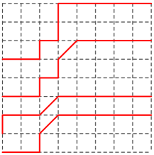
We construct a weight preserving bijection between reverse plane overpartitions and sets of nonintersecting paths on a triangular lattice in a similar fashion as in Section 3.1. The lattice consists of East, North and North–East edges. East edges have weight 111, North edges on (vertical) level i𝑖i have weight qi+1superscript𝑞𝑖1q^{i+1} and North–East edges joining vertical levels i𝑖i and i+1𝑖1i+1 have weight qi+1superscript𝑞𝑖1q^{i+1}. The weight of a set of nonintersecting paths p𝑝p is the product of the weights of their edges and is denoted by w(p)𝑤𝑝w(p). Let ΠΠ\Pi be a reverse plane overpartition whose positive entries form a skew shape λ/μ𝜆𝜇\lambda/\mu and let =(λ)𝜆\ell=\ell(\lambda). Then ΠΠ\Pi can be represented by a set of n𝑛n nonintersecting lattice paths such that

  • the departure points are (0,μi+i)0subscript𝜇𝑖𝑖(0,\mu_{i}+\ell-i) and

  • the arrivals points are (x,λi+i)𝑥subscript𝜆𝑖𝑖(x,\lambda_{i}+\ell-i),

for a large enough x𝑥x and i=1,,𝑖1i=1,\dots,\ell. For example let x=8𝑥8x=8, λ=(5,4,2,2)𝜆5422\lambda=(5,4,2,2) and μ=(2,1)𝜇21\mu=(2,1). Figure 6 shows the corresponding set of nonintersecting paths for the reverse plane overpartition of shape λ/μ𝜆𝜇\lambda/\mu
344344¯13¯33¯.missing-subexpressionmissing-subexpression344missing-subexpressionmissing-subexpression34¯4missing-subexpressionmissing-subexpression1¯3missing-subexpressionmissing-subexpressionmissing-subexpressionmissing-subexpression3¯3missing-subexpressionmissing-subexpressionmissing-subexpressionmissing-subexpression\begin{array}[]{llllll}&&{3}&4&4&\\ &3&{4}&\bar{4}&\\ 1&\bar{3}&&&&\\ 3&\bar{3}&&&\end{array}.
Refer to caption
Figure 6. Nonintersecting paths and reverse plane overpartitions

This implies that all reverse plane overpartitions of shape λ=(λ1,,λ)𝜆subscript𝜆1subscript𝜆\lambda=(\lambda_{1},\ldots,\lambda_{\ell}) can be represented by nonintersecting lattice paths such that

  • the departure points are an \ell–element subset of {(0,i)|i0}conditional-set0𝑖𝑖0\{(0,i)\ |i\geq 0\} and

  • the arrivals points are (x,λi+i),𝑥subscript𝜆𝑖𝑖(x,\lambda_{i}+\ell-i),

with x𝑥x\rightarrow\infty.

Now, for r1>r2>>r0subscript𝑟1subscript𝑟2subscript𝑟0r_{1}>r_{2}>\dots>r_{\ell}\geq 0 we define

W(r1,r2,,r)=limxpP(x;r1,,r)w(p),𝑊subscript𝑟1subscript𝑟2subscript𝑟subscript𝑥subscript𝑝𝑃𝑥subscript𝑟1subscript𝑟𝑤𝑝W(r_{1},r_{2},\dots,r_{\ell})=\lim_{x\to\infty}\sum_{p\in P(x;r_{1},\dots,r_{\ell})}w(p),

where P(x;r1,r2,,r)𝑃𝑥subscript𝑟1subscript𝑟2subscript𝑟P(x;r_{1},r_{2},\dots,r_{\ell}) is the set of all nonintersecting paths joining an \ell-element subset of {(0,i)|i0}conditional-set0𝑖𝑖0\{(0,i)|i\geq 0\} with {(x,r1),,(x,r)}𝑥subscript𝑟1𝑥subscript𝑟\{(x,r_{1}),\dots,(x,r_{\ell})\}. Note that for r1>r2>>r>0subscript𝑟1subscript𝑟2subscript𝑟0r_{1}>r_{2}>\dots>r_{\ell}>0 we have

(3.6) W(r1,,r,0)=W(r11,,r1).𝑊subscript𝑟1subscript𝑟0𝑊subscript𝑟11subscript𝑟1W(r_{1},\dots,r_{\ell},0)=W(r_{1}-1,\dots,r_{\ell}-1).

By Stembridge’s Pfaffian formula for the sum of the weights of nonintersecting paths where departure points are not fixed (Theorem 3.1 of [Ste]) we obtain

W(r1,r2,,r)=Pf(D),𝑊subscript𝑟1subscript𝑟2subscript𝑟Pf𝐷W(r_{1},r_{2},\dots,r_{\ell})=\text{Pf}(D),

where if \ell is even D𝐷D is the ×\ell\times\ell skew–symmetric matrix defined by Di,j=W(ri,rj)subscript𝐷𝑖𝑗𝑊subscript𝑟𝑖subscript𝑟𝑗D_{i,j}=W(r_{i},r_{j}) for 1i<j1𝑖𝑗1\leq i<j\leq\ell and if \ell is odd D𝐷D is the (+1)×(+1)11(\ell+1)\times(\ell+1) skew–symmetric matrix defined by Di,j=W(ri,rj)subscript𝐷𝑖𝑗𝑊subscript𝑟𝑖subscript𝑟𝑗D_{i,j}=W(r_{i},r_{j}) for 1i<j1𝑖𝑗1\leq i<j\leq\ell and Di,+1=W(ri)subscript𝐷𝑖1𝑊subscript𝑟𝑖D_{i,\ell+1}=W(r_{i}) for 1i1𝑖1\leq i\leq\ell.

Lemma 2.

Let r>s0𝑟𝑠0r>s\geq 0. Then

(3.7) W(s)𝑊𝑠\displaystyle W(s) =\displaystyle= (q)s(q)s,subscript𝑞𝑠subscript𝑞𝑠\displaystyle\frac{(-q)_{s}}{(q)_{s}},
(3.8) W(r,s)𝑊𝑟𝑠\displaystyle W(r,s) =\displaystyle= (q)r(q)r(q)s(q)s1qrs1+qrs.subscript𝑞𝑟subscript𝑞𝑟subscript𝑞𝑠subscript𝑞𝑠1superscript𝑞𝑟𝑠1superscript𝑞𝑟𝑠\displaystyle\frac{(-q)_{r}}{(q)_{r}}\cdot\frac{(-q)_{s}}{(q)_{s}}\cdot\frac{1-q^{r-s}}{1+q^{r-s}}.
Proof.

From Lemma 1 we have that the generating function for overpartitions with at most n𝑛n parts is M(n)=(q)n/(q)n𝑀𝑛subscript𝑞𝑛subscript𝑞𝑛M(n)=(-q)_{n}/(q)_{n} and the generating function for overpartitions with exactly n𝑛n parts is P(n)=qn(1)n/(q)n𝑃𝑛superscript𝑞𝑛subscript1𝑛subscript𝑞𝑛P(n)=q^{n}(-1)_{n}/(q)_{n}. This implies that

(3.9) i=0nP(i)=M(n).superscriptsubscript𝑖0𝑛𝑃𝑖𝑀𝑛\sum_{i=0}^{n}P(i)=M(n).

Moreover,

W(s)=M(s)=(q)s(q)sandW(r,0)=M(r1)=(q)r1(q)r1.formulae-sequence𝑊𝑠𝑀𝑠subscript𝑞𝑠subscript𝑞𝑠and𝑊𝑟0𝑀𝑟1subscript𝑞𝑟1subscript𝑞𝑟1W(s)=M(s)=\frac{(-q)_{s}}{(q)_{s}}\;\;\;\;\;\text{and}\;\;\;\;\;W(r,0)=M(r-1)=\frac{(-q)_{r-1}}{(q)_{r-1}}.

We prove (3.8) by induction on s𝑠s. The formula for the base case s=0𝑠0s=0 holds by the above. So, we assume s1𝑠1s\geq 1.

By Lindström’s determinantal formula (Lemma 1 of [Li]) we have that

W(r,s)=i=0sj=i+1r(P(rj)P(si)P(ri)P(sj)).𝑊𝑟𝑠superscriptsubscript𝑖0𝑠superscriptsubscript𝑗𝑖1𝑟𝑃𝑟𝑗𝑃𝑠𝑖𝑃𝑟𝑖𝑃𝑠𝑗W(r,s)=\sum_{i=0}^{s}\sum_{j=i+1}^{r}\left(P(r-j)P(s-i)-P(r-i)P(s-j)\right).

Summing over j𝑗j and using (3.9) we obtain

W(r,s)=i=0s(P(si)M(ri1)P(ri)M(s1i)).𝑊𝑟𝑠superscriptsubscript𝑖0𝑠𝑃𝑠𝑖𝑀𝑟𝑖1𝑃𝑟𝑖𝑀𝑠1𝑖W(r,s)=\sum_{i=0}^{s}\left(P(s-i)M(r-i-1)-P(r-i)M(s-1-i)\right).

Then

W(r,s)=W(r1,s1)+P(s)M(r1)P(r)M(s1).𝑊𝑟𝑠𝑊𝑟1𝑠1𝑃𝑠𝑀𝑟1𝑃𝑟𝑀𝑠1W(r,s)=W(r-1,s-1)+P(s)M(r-1)-P(r)M(s-1).

It is enough to prove that

(3.10) P(s)M(r1)P(r)M(s1)W(r1,s1)=2(qr+qs)(1qr)(1qs)𝑃𝑠𝑀𝑟1𝑃𝑟𝑀𝑠1𝑊𝑟1𝑠12superscript𝑞𝑟superscript𝑞𝑠1superscript𝑞𝑟1superscript𝑞𝑠\frac{P(s)M(r-1)-P(r)M(s-1)}{W(r-1,s-1)}=\frac{2(q^{r}+q^{s})}{(1-q^{r})(1-q^{s})}

and (3.8) follows by induction. Now,

P(s)M(r1)P(r)M(s1)=𝑃𝑠𝑀𝑟1𝑃𝑟𝑀𝑠1absent\displaystyle P(s)M(r-1)-P(r)M(s-1)=
=qs(1)s(q)s(q)r1(q)r1qr(1)r(q)r(q)s1(q)s1absentsuperscript𝑞𝑠subscript1𝑠subscript𝑞𝑠subscript𝑞𝑟1subscript𝑞𝑟1superscript𝑞𝑟subscript1𝑟subscript𝑞𝑟subscript𝑞𝑠1subscript𝑞𝑠1\displaystyle=q^{s}\frac{(-1)_{s}}{(q)_{s}}\cdot\frac{(-q)_{r-1}}{(q)_{r-1}}-q^{r}\frac{(-1)_{r}}{(q)_{r}}\cdot\frac{(-q)_{s-1}}{(q)_{s-1}}
=(q)r1(q)r1(q)s1(q)s11+qrs1qrs2(qr+qs)(1qr)(1qs).absentsubscript𝑞𝑟1subscript𝑞𝑟1subscript𝑞𝑠1subscript𝑞𝑠11superscript𝑞𝑟𝑠1superscript𝑞𝑟𝑠2superscript𝑞𝑟superscript𝑞𝑠1superscript𝑞𝑟1superscript𝑞𝑠\displaystyle=\frac{(-q)_{r-1}}{(q)_{r-1}}\cdot\frac{(-q)_{s-1}}{(q)_{s-1}}\cdot\frac{1+q^{r-s}}{1-q^{r-s}}\cdot\frac{2(q^{r}+q^{s})}{(1-q^{r})(1-q^{s})}.

Using the inductive hypothesis for W(r1,s1)𝑊𝑟1𝑠1W(r-1,s-1) we obtain (3.10).

Let Fλsubscript𝐹𝜆F_{\lambda} be the generating function for reverse plane overpartitions of shape λ𝜆\lambda. Then, using the bijection we have constructed, we obtain

Fλ=W(λ1+1,λ2+2,,λ),subscript𝐹𝜆𝑊subscript𝜆11subscript𝜆22subscript𝜆F_{\lambda}=W(\lambda_{1}+\ell-1,\lambda_{2}+\ell-2,\dots,\lambda_{\ell}),

which, after applying Stembridge’s result, gives us a Pfaffian formula. This Pfaffian formula can be expressed as a product after the following observations.

Let M be 2n×2n2𝑛2𝑛2n\times 2n skew–symmetric matrix. One of definitions of the Pfaffian is the following:

Pf(M)=π=(i1,j1)(in,jn)sgn(π)Mi1,j1Mi2,j2Min,jn,Pf𝑀subscript𝜋subscript𝑖1subscript𝑗1subscript𝑖𝑛subscript𝑗𝑛sgn𝜋subscript𝑀subscript𝑖1subscript𝑗1subscript𝑀subscript𝑖2subscript𝑗2subscript𝑀subscript𝑖𝑛subscript𝑗𝑛\text{Pf}(M)=\sum_{\pi=(i_{1},j_{1})\ldots(i_{n},j_{n})}\text{sgn}(\pi)M_{i_{1},j_{1}}M_{i_{2},j_{2}}\cdots M_{i_{n},j_{n}},

where the sum is over all of perfect matchings (or fixed point free involutions) of [2n]delimited-[]2𝑛[2n]. Also, for r>s>0𝑟𝑠0r>s>0,

W(s)𝑊𝑠\displaystyle W(s) =\displaystyle= 1+qs1qsW(s1),1superscript𝑞𝑠1superscript𝑞𝑠𝑊𝑠1\displaystyle\frac{1+q^{s}}{1-q^{s}}W(s-1),
andW(r,s)and𝑊𝑟𝑠\displaystyle{\rm and}\ \ W(r,s) =\displaystyle= 1+qr1qr1+qs1qsW(r1,s1).1superscript𝑞𝑟1superscript𝑞𝑟1superscript𝑞𝑠1superscript𝑞𝑠𝑊𝑟1𝑠1\displaystyle\frac{1+q^{r}}{1-q^{r}}\cdot\frac{1+q^{s}}{1-q^{s}}W(r-1,s-1).

Then

Fλ=j=11+qhj,11qhj,1Fλ¯,subscript𝐹𝜆superscriptsubscriptproduct𝑗11superscript𝑞subscript𝑗11superscript𝑞subscript𝑗1subscript𝐹¯𝜆F_{\lambda}=\prod_{j=1}^{\ell}\frac{1+q^{h_{j,1}}}{1-q^{h_{j,1}}}\cdot F_{\bar{\lambda}},

where λ¯=(λ11,,λ1)¯𝜆subscript𝜆11subscript𝜆1\bar{\lambda}=(\lambda_{1}-1,\dots,\lambda_{\ell}-1) if λ>1subscript𝜆1\lambda_{\ell}>1 and λ¯=(λ11,,λ11)¯𝜆subscript𝜆11subscript𝜆11\bar{\lambda}=(\lambda_{1}-1,\dots,\lambda_{\ell-1}-1) if λ=1subscript𝜆1\lambda_{\ell}=1 (see (3.6) in this case). Inductively we obtain Theorem 9.

4. Domino tilings

In [V1] a measure on (diagonally) strict plane partitions was studied. Strict plane partitions are plane partitions were all diagonals are strict partitions, i.e. strictly decreasing sequences. They can also be seen as plane overpartitions where all overlines are deleted. There are 2k(Π)superscript2𝑘Π2^{k(\Pi)} different plane overpartitions corresponding to the same strict plane partition ΠΠ\Pi, where k(Π)𝑘Πk(\Pi) is the number of connected components of ΠΠ\Pi.

Alternatively, a strict plane partition can be seen as a subset of ×\mathbb{N}\times\mathbb{Z} consisting of points (t,x)𝑡𝑥(t,x) where x𝑥x is a part of the diagonal partition indexed by t𝑡t. See Figure 7. We call this set the 2-dimensional diagram of that strict plane partition. The connected components are connected sets (no holes) on the same horizontal line. The 2-dimensional diagram of a plane overpartition is the 2-dimensional diagram of its corresponding strict plane partition.
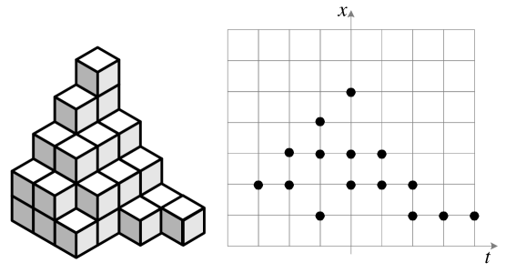
Refer to caption
Figure 7. A strict plane partition and its corresponding 2-dimensional diagram

The measure studied in [V1] assigns to each strict plane partition a weight equal to 2k(Π)q|Π|superscript2𝑘Πsuperscript𝑞Π2^{k(\Pi)}q^{|\Pi|}. The limit shape of this measure is given in terms of the Ronkin function of the polynomial P(z,w)=1+z+w+zw𝑃𝑧𝑤1𝑧𝑤𝑧𝑤P(z,w)=-1+z+w+zw and it is parameterized on the domain representing half of the amoeba of this polynomial. This polynomial is also related to plane tilings with dominoes. This, as well as some other features like similarities in correlation kernels [J, V1] suggested that a connection between this measure and domino tilings is likely to exist.

Alternatively, one can see this measure as a uniform measure on plane overpartitions, i.e. each plane overpartition ΠΠ\Pi has a probability proportional to q|Π|superscript𝑞Πq^{|\Pi|}. In Section 3 we have constructed a bijection between plane overpartitions and sets of nonintersecting paths. See Figure 8. This figure is obtained from Figure 5 by a rotation. Note that the paths are incident with all points in the corresponding 2-dimensional diagram. The paths consist of edges of three different kinds: horizontal (joining (t,x)𝑡𝑥(t,x) and (t+1,x)𝑡1𝑥(t+1,x)), vertical (joining (t,x+1)𝑡𝑥1(t,x+1) and (t,x)𝑡𝑥(t,x)) and diagonal (joining (t,x+1)𝑡𝑥1(t,x+1) and (t+1,x)𝑡1𝑥(t+1,x)). There is a standard way to construct a tiling with dominoes using these paths(see for example [J]). We explain the process below. An example is given on Figure 8.
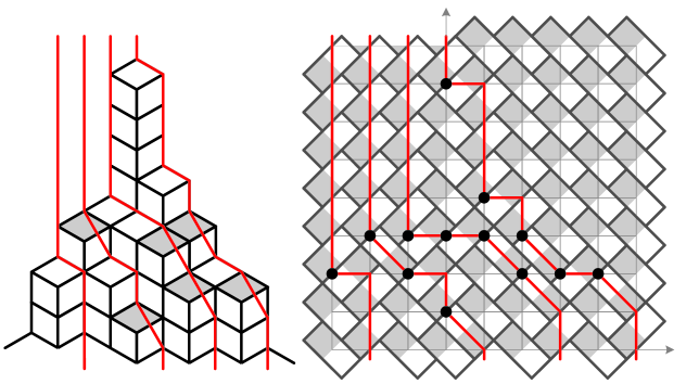
Refer to caption
Figure 8. A plane overpartition and its corresponding domino tiling

We start from 2superscript2\mathbb{R}^{2} and color it in a chessboard fashion such that (1/4,1/4)1414(1/4,1/4), (1/4,3/4)1434(-1/4,3/4), (1/4,5/4)1454(1/4,5/4) and (3/4,3/4)3434(3/4,3/4) are vertices of a white square. So, the axes of this infinite chessboard form angles of 454545 and 135135135 degrees with the axes of 2superscript2\mathbb{R}^{2}. A domino placed on this infinite chessboard can be one of the four types: (1,1)11(1,1), (1,1)11(-1,-1), (1,1)11(-1,1) or (1,1)11(1,-1), where we say that a domino is of type (x,y)𝑥𝑦(x,y) if (x,y)𝑥𝑦(x,y) is the vector parallel to the vector whose starting, respectively end point is the center of the white, respectively black square of that domino.

Now, take a plane overpartition and represent it on this chessboard by its corresponding set of nonintersecting paths. We cover each edge by a domino that satisfies that the endpoints of that edge are midpoints of sides of the black and white square of that domino. In that way, we obtain a tiling of a part of the plane with dominoes of three types: (1,1)11(1,1), (1,1)11(-1,-1) and (1,1)11(1,-1). More precisely, horizontal edges correspond to (1,1)11(1,1) dominoes, vertical to (1,1)11(-1,-1) and diagonal to (1,1)11(1,-1). To tile the whole plane we fill the rest of it by dominoes of the fourth, (1,1)11(-1,1) type. See Figure 8 for an illustration.

In this way, we have established a correspondence between plane overpartitions and plane tilings with dominoes. We now give some of the properties of this correspondence. First, we describe how a tiling changes when we add or remove an overline or we add or remove a box from a plane overpartition. We require that when we add/remove an overline or a box we obtain a plane overpartition again.

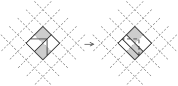
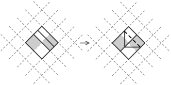
In terms of the 2-dimensional diagram of a plane partition, adding an overline can occur at all places where (t,x)𝑡𝑥(t,x) is in the diagram and (t+1,x)𝑡1𝑥(t+1,x) is not. Adding an overline at (t,x)𝑡𝑥(t,x) means that a pair of horizontal and vertical edges, ((t,x),(t+1,x))𝑡𝑥𝑡1𝑥((t,x),(t+1,x)) and ((t+1,x),(t+1,x1))𝑡1𝑥𝑡1𝑥1((t+1,x),(t+1,x-1)), is replaced by one diagonal edge, ((t,x),(t+1,x1))𝑡𝑥𝑡1𝑥1((t,x),(t+1,x-1)). This means that the new tiling differs from the old one by replacing a pair of (1,1)11(1,1) and (1,1)11(-1,-1) dominoes by a pair of (1,1)11(1,-1) and (1,1)11(-1,1) dominoes. See Figure 9.

Refer to caption
Figure 9. Adding an overline

Removing an overline is the inverse of adding an overline.

We now explain the operation of removing a box. Observe that if a box can be removed from a plane overpartition then the corresponding part is overlined or it can be overlined to obtain a plane overpartition again. So, it is enough to consider how the tiling changes when we remove an overlined box since we have already considered the case of adding or removing an overline. If we remove an overlined box we change a diagonal edge to a pair of vertical and horizontal edges. If the box was represented by (t,x)𝑡𝑥(t,x) in the 2-dimensional diagram then the edge ((t,x),(t+1,x1))𝑡𝑥𝑡1𝑥1((t,x),(t+1,x-1)) is replaced by the pair of ((t,x),(t,x1))𝑡𝑥𝑡𝑥1((t,x),(t,x-1)) and ((t,x1),(t+1,x1))𝑡𝑥1𝑡1𝑥1((t,x-1),(t+1,x-1)). This means that the new tiling differs from the old one by replacing a pair of (1,1)11(1,-1) and (1,1)11(-1,1) dominoes by a pair of (1,1)11(1,1) and (1,1)11(-1,-1) dominoes. See Figure 10.

Refer to caption
Figure 10. Removing a box

All four operations are described by a swap of a pair of adjacent (1,1)11(1,1) and (1,1)11(-1,-1) dominoes and a pair of adjacent of (1,1)11(1,-1) and (1,1)11(-1,1) dominoes.

We conclude this section by the observation that plane overpartitions of a given shape λ𝜆\lambda and whose parts are bounded by n𝑛n are in bijection with domino tilings of the rectangle [(λ)+1,λ1]×[0,n]𝜆1subscript𝜆10𝑛[-\ell(\lambda)+1,\lambda_{1}]\times[0,n] with certain boundary conditions. These conditions are imposed by the fact that outside of this rectangle nonintersecting paths are just straight lines. We describe the boundary conditions precisely in the proposition below.

Proposition 5.

The set 𝒮(λ)(n)𝒮𝜆𝑛\mathcal{S}(\lambda)\cap\mathcal{L}(n) of all plane overpartitions of shape λ𝜆\lambda and whose largest part is at most n is in bijection with plane tilings with dominoes where a point (t,x)×𝑡𝑥(t,x)\in\mathbb{Z}\times\mathbb{R} is covered by a domino of type (1,1)11(-1,-1) if

  • t(λ),𝑡𝜆t\leq-\ell(\lambda),

  • (λ)<t0𝜆𝑡0-\ell(\lambda)<t\leq 0 and xn,𝑥𝑛x\geq n,

  • t=λii+1𝑡subscript𝜆𝑖𝑖1t=\lambda_{i}-i+1 for some i𝑖i and x0,𝑥0x\leq 0,

and a domino of type (1,1)11(-1,1) if

  • t>λ1,𝑡subscript𝜆1t>\lambda_{1},

  • 0<tλ10𝑡subscript𝜆10<t\leq\lambda_{1} and xn+1/2,𝑥𝑛12x\geq n+1/2,

  • tλii+1𝑡subscript𝜆𝑖𝑖1t\neq\lambda_{i}-i+1 for all i𝑖i and x1/2.𝑥12x\leq-1/2.

The boundary conditions for λ=(5,4,3,1)𝜆5431\lambda=(5,4,3,1) and n=7𝑛7n=7 are shown in Figure 11. The example from Figure 8 satisfies these boundary conditions.
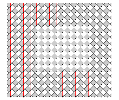
Refer to caption
Figure 11. Boundary conditions

5. Robinson-Schensted-Knuth (RSK) type algorithm for plane overpartitions

In this section we are going to give a bijection between certain matrices and pairs of plane overpartitions of the same shape. This bijection is obtained by an algorithm similar to the algorithm RS2 of Berele and Remmel [BeR] which gives a bijection between matrices and pairs of (k,)𝑘(k,\ell)-semistandard tableaux. These tableaux are super semistandard tableaux, defined in Section 3, where the nonoverlined (resp. overlined) parts are less than or equal to k𝑘k (resp. \ell).

We then apply properties of this algorithm to enumerate plane overpartitions, as done by Bender and Knuth [BK] for plane partitions.

5.1. The RSK algorithm

Let M=(ABCD)𝑀matrix𝐴𝐵𝐶𝐷M=\begin{pmatrix}A&B\\ C&D\end{pmatrix} be a 2n×2n2𝑛2𝑛2n\times 2n matrix, made of four n×n𝑛𝑛n\times n blocks A,B,C𝐴𝐵𝐶A,B,C and D𝐷D. The blocks A𝐴A and D𝐷D are nonnegative integer matrices, and B𝐵B and C𝐶C are {0,1}01\left\{0,1\right\} matrices. We denote the set of all such matrices with nsubscript𝑛\mathcal{M}_{n}. We represent a matrix in nsubscript𝑛\mathcal{M}_{n} by a sequence of pairs of numbers (ij)matrix𝑖𝑗\begin{pmatrix}i\\ j\end{pmatrix}, (ij¯)matrix𝑖¯𝑗\begin{pmatrix}i\\ \bar{j}\end{pmatrix}, (i¯j)matrix¯𝑖𝑗\begin{pmatrix}\bar{i}\\ j\end{pmatrix} and (i¯j¯)matrix¯𝑖¯𝑗\begin{pmatrix}\bar{i}\\ \bar{j}\end{pmatrix}.

The encoding of M𝑀M into pairs is made using the following rules:

  • for each nonzero entry aijsubscript𝑎𝑖𝑗a_{ij} of A𝐴A, we create aijsubscript𝑎𝑖𝑗a_{ij} pairs (ij)matrix𝑖𝑗\begin{pmatrix}i\\ j\end{pmatrix},

  • for each nonzero entry bijsubscript𝑏𝑖𝑗b_{ij} of B𝐵B, we create one pair (ij¯)matrix𝑖¯𝑗\begin{pmatrix}i\\ \bar{j}\end{pmatrix},

  • for each nonzero entry cijsubscript𝑐𝑖𝑗c_{ij} of C𝐶C, we create one pair (i¯j)matrix¯𝑖𝑗\begin{pmatrix}\bar{i}\\ j\end{pmatrix},

  • for each nonzero entry dijsubscript𝑑𝑖𝑗d_{ij} of D𝐷D, we create dijsubscript𝑑𝑖𝑗d_{ij} pairs (i¯j¯)matrix¯𝑖¯𝑗\begin{pmatrix}\bar{i}\\ \bar{j}\end{pmatrix}.

For example let M=(0210201011010011)𝑀matrix0210201011010011M=\begin{pmatrix}0&2&1&0\\ 2&0&1&0\\ 1&1&0&1\\ 0&0&1&1\end{pmatrix}. After encoding M𝑀M, we obtain

(12),(12),(11¯),(21),(21),(21¯),(1¯1),(1¯2),(1¯2¯),(2¯1¯),(2¯2¯).matrix12matrix12matrix1¯1matrix21matrix21matrix2¯1matrix¯11matrix¯12matrix¯1¯2matrix¯2¯1matrix¯2¯2\begin{pmatrix}1\\ 2\end{pmatrix},\begin{pmatrix}1\\ 2\end{pmatrix},\begin{pmatrix}1\\ \bar{1}\end{pmatrix},\begin{pmatrix}2\\ 1\end{pmatrix},\begin{pmatrix}2\\ 1\end{pmatrix},\begin{pmatrix}2\\ \bar{1}\end{pmatrix},\begin{pmatrix}\bar{1}\\ 1\end{pmatrix},\begin{pmatrix}\bar{1}\\ 2\end{pmatrix},\begin{pmatrix}\bar{1}\\ \bar{2}\end{pmatrix},\begin{pmatrix}\bar{2}\\ \bar{1}\end{pmatrix},\begin{pmatrix}\bar{2}\\ \bar{2}\end{pmatrix}.

From now on, we fix the order 1¯<1<2¯<2<3¯<3<¯11¯22¯33\bar{1}<1<\bar{2}<2<\bar{3}<3<.... We sort the pairs to create a two–line array L𝐿L such that

  • the first line is a nonincreasing sequence,

  • if two entries of the first line are equal and overlined (resp. nonoverlined) then the corresponding entries in the second line are in weakly increasing (resp. decreasing) order.

For the example above, after sorting, we obtain the two–line array

L=(2,2,2,2¯,2¯,1,1,1,1¯,1¯,1¯1,1,1¯,1¯,2¯,2,2,1¯,1,2¯,2).𝐿matrix222¯2¯2111¯1¯1¯111¯1¯1¯222¯11¯22L=\begin{pmatrix}2,2,2,\bar{2},\bar{2},1,1,1,\bar{1},\bar{1},\bar{1}\\ 1,1,\bar{1},\bar{1},\bar{2},2,2,\bar{1},1,\bar{2},2\end{pmatrix}.

We now describe the insertion algorithm. It is based on an algorithm proposed by Knuth in [K] and quite similar to the algorithm RS2 of [BeR].

We first explain how to insert a number j𝑗j into an overpartition λ𝜆\lambda of length \ell, so that the sequence λ𝜆\lambda is still an overpartition. If j𝑗j can be inserted at the end of λ𝜆\lambda, then insert and stop. Otherwise, find the smallest part that can be replaced by j𝑗j. Bump this part and insert j𝑗j. At the end we obtain a new overpartition that contains j𝑗j as a part and whose length is \ell if we bumped a part or +11\ell+1 if j𝑗j was added at the end and no part was bumped. For example if λ=(4,3,3,3¯,2)𝜆433¯32\lambda=(4,3,3,\bar{3},2) then

  • insert 5, obtain (5,3,3,3¯,2)533¯32(5,3,3,\bar{3},2) and bump 4,

  • insert 3, obtain (4,3,3,3,2)43332(4,3,3,3,2) and bump 3¯¯3\bar{3},

  • insert 3¯¯3\bar{3}, obtain (4,3,3,3¯,2)433¯32(4,3,3,\bar{3},2) and bump 3¯¯3\bar{3},

  • insert 1, obtain (4,3,3,3¯,2,1)433¯321(4,3,3,\bar{3},2,1) and bump nothing.

To insert j𝑗j into a plane overpartition P𝑃P insert j𝑗j in the first row. If nothing is bumped then stop. Otherwise, insert the bumped part in the second row. If something is bumped from the second row, insert it in the third and so on. Stop when nothing is bumped. For example when 3¯¯3\bar{3} is inserted in

4333¯233¯21we obtain4333¯233¯23¯1.433¯323¯32missing-subexpressionmissing-subexpression1missing-subexpressionmissing-subexpressionmissing-subexpressionmissing-subexpressionwe obtain433¯323¯32missing-subexpressionmissing-subexpression¯3missing-subexpressionmissing-subexpressionmissing-subexpressionmissing-subexpression1missing-subexpressionmissing-subexpressionmissing-subexpressionmissing-subexpression\begin{array}[]{lllll}4&3&3&\bar{3}&2\\ 3&\bar{3}&2&\\ 1&&&&\\ \end{array}\quad\textrm{we obtain}\quad\begin{array}[]{lllll}4&3&3&\bar{3}&2\\ 3&\bar{3}&2&\\ \bar{3}&&&&\\ 1&&&&\\ \end{array}.

We define how to insert a pair (ij)matrix𝑖𝑗\begin{pmatrix}i\\ j\end{pmatrix} into a pair of plane overpartitions of the same shape (P,Q)𝑃𝑄(P,Q). We first insert j𝑗j in P𝑃P with the insertion algorithm. If the insertion ends in column c𝑐c and row r𝑟r of P𝑃P, then insert i𝑖i in column c𝑐c and row r𝑟r in Q𝑄Q. Finally going from the two–line array L𝐿L to pairs of plane overpartitions of the same shape works as follows: start with two empty plane overpartitions and insert each pair of L𝐿L going from left to right. This is identical to the classical RSK algorithm [K].

Continuing with the previous example and applying the insertion algorithm we get

P=2222¯112¯1¯11¯1¯,Q=2222¯112¯1¯11¯1¯.formulae-sequence𝑃222¯211¯2¯1missing-subexpression1missing-subexpressionmissing-subexpression¯1missing-subexpressionmissing-subexpression¯1missing-subexpressionmissing-subexpression𝑄222¯211¯2¯1missing-subexpression1missing-subexpressionmissing-subexpression¯1missing-subexpressionmissing-subexpression¯1missing-subexpressionmissing-subexpressionmissing-subexpression\begin{array}[]{ll}P=\begin{array}[]{lll}2&2&2\\ \bar{2}&1&1\\ \bar{2}&\bar{1}&\\ 1&&\\ \bar{1}&&\\ \bar{1}&&\end{array},\ \ \ \ \ \ Q=\begin{array}[]{lll}2&2&2\\ \bar{2}&1&1\\ \bar{2}&\bar{1}&\\ 1&&\\ \bar{1}&&\\ \bar{1}&&\end{array}\end{array}.

Let (n)𝑛\mathcal{L}(n) be the set of all plane overpartitions with the largest entry at most n𝑛n.

Theorem 10.

There is a one-to-one correspondence between matrices Mn𝑀subscript𝑛M\in\mathcal{M}_{n} and pairs of plane overpartitions of the same shape (P,Q)(n)×(n)𝑃𝑄𝑛𝑛(P,Q)\in\mathcal{L}(n)\times\mathcal{L}(n). This correspondence is such that :

  • k𝑘k appears in P𝑃P exactly iaik+ciksubscript𝑖subscript𝑎𝑖𝑘subscript𝑐𝑖𝑘\sum_{i}a_{ik}+c_{ik} times,

  • k¯¯𝑘\bar{k} appears in P𝑃P exactly ibik+diksubscript𝑖subscript𝑏𝑖𝑘subscript𝑑𝑖𝑘\sum_{i}b_{ik}+d_{ik} times,

  • k𝑘k appears in Q𝑄Q exactly iaik+biksubscript𝑖subscript𝑎𝑖𝑘subscript𝑏𝑖𝑘\sum_{i}a_{ik}+b_{ik} times,

  • k¯¯𝑘\bar{k} appears in Q𝑄Q exactly icik+diksubscript𝑖subscript𝑐𝑖𝑘subscript𝑑𝑖𝑘\sum_{i}c_{ik}+d_{ik} times.

Proof.

The proof is identical to the proof in the case of the RSK algorithm [K] or the RS2 algorithm [BeR]. Details are given in [Sav]. ∎

Theorem 11.

If the insertion algorithm produces (P,Q)𝑃𝑄(P,Q) with input matrix M𝑀M, then the insertion algorithm produces (Q,P)𝑄𝑃(Q,P) with input matrix MTsuperscript𝑀𝑇M^{T}.

Proof.

The proof is again analogous to the one in [K]. Given a two–line array (u1,,uNv1,,vN)matrixsubscript𝑢1subscript𝑢𝑁subscript𝑣1subscript𝑣𝑁\begin{pmatrix}u_{1},\ldots,u_{N}\\ v_{1},\ldots,v_{N}\end{pmatrix}, we partition the pairs (uv)matrixsubscript𝑢subscript𝑣\begin{pmatrix}u_{\ell}\\ v_{\ell}\end{pmatrix} in classes such that (ukvk)matrixsubscript𝑢𝑘subscript𝑣𝑘\begin{pmatrix}u_{k}\\ v_{k}\end{pmatrix} and (umvm)matrixsubscript𝑢𝑚subscript𝑣𝑚\begin{pmatrix}u_{m}\\ v_{m}\end{pmatrix} are in the same class if and only if :

  • ukumsubscript𝑢𝑘subscript𝑢𝑚u_{k}\geq u_{m} and if uk=umsubscript𝑢𝑘subscript𝑢𝑚u_{k}=u_{m}, then umsubscript𝑢𝑚u_{m} is overlined AND

  • vkvmsubscript𝑣𝑘subscript𝑣𝑚v_{k}\leq v_{m} and if vk=vmsubscript𝑣𝑘subscript𝑣𝑚v_{k}=v_{m}, then vksubscript𝑣𝑘v_{k} is overlined.

Then one can sort each class so that the first entries of each pair appear in nonincreasing order and then sort the classes so that the first entries of the first pair of each class are in nonincreasing order. For example if the two–line array is

(2,2,2,2¯,2¯,1,1,1,1¯,1¯,1¯1,1,1¯,1¯,2¯,2,2,1¯,1,2¯,2)matrix222¯2¯2111¯1¯1¯111¯1¯1¯222¯11¯22\begin{pmatrix}2,2,2,\bar{2},\bar{2},1,1,1,\bar{1},\bar{1},\bar{1}\\ 1,1,\bar{1},\bar{1},\bar{2},2,2,\bar{1},1,\bar{2},2\end{pmatrix},

we get the classes

C1={(21),(2¯2¯),(12)},C2={(21),(12)},formulae-sequencesubscript𝐶1matrix21matrix¯2¯2matrix12subscript𝐶2matrix21matrix12C_{1}=\left\{\begin{pmatrix}2\\ 1\end{pmatrix},\begin{pmatrix}\bar{2}\\ \bar{2}\end{pmatrix},\begin{pmatrix}1\\ 2\end{pmatrix}\right\},\ \ C_{2}=\left\{\begin{pmatrix}2\\ 1\end{pmatrix},\begin{pmatrix}{1}\\ {2}\end{pmatrix}\right\},\ \
C3={(21¯),(2¯1¯),(11¯),(1¯1),(1¯2¯),(1¯2)}.subscript𝐶3matrix2¯1matrix¯2¯1matrix1¯1matrix¯11matrix¯1¯2matrix¯12C_{3}=\left\{\begin{pmatrix}2\\ \bar{1}\end{pmatrix},\begin{pmatrix}\bar{2}\\ \bar{1}\end{pmatrix},\begin{pmatrix}1\\ \bar{1}\end{pmatrix},\begin{pmatrix}\bar{1}\\ 1\end{pmatrix},\begin{pmatrix}\bar{1}\\ \bar{2}\end{pmatrix},\begin{pmatrix}\bar{1}\\ 2\end{pmatrix}\right\}.\ \

If the classes are C1,,Cdsubscript𝐶1subscript𝐶𝑑C_{1},\ldots,C_{d} with

Ci={(ui1vi1),,(uinivini)}subscript𝐶𝑖matrixsubscript𝑢𝑖1subscript𝑣𝑖1matrixsubscript𝑢𝑖subscript𝑛𝑖subscript𝑣𝑖subscript𝑛𝑖C_{i}=\left\{\begin{pmatrix}u_{i1}\\ v_{i1}\end{pmatrix},\ldots,\begin{pmatrix}u_{in_{i}}\\ v_{in_{i}}\end{pmatrix}\right\}

then the first row of P𝑃P is

v1n1,,vdndsubscript𝑣1subscript𝑛1subscript𝑣𝑑subscript𝑛𝑑v_{1n_{1}},\ldots,v_{dn_{d}}

and the first row of Q𝑄Q is

u11,,ud1.subscript𝑢11subscript𝑢𝑑1u_{11},\ldots,u_{d1}.

Moreover one constructs the rest of P𝑃P and Q𝑄Q using the pairs :

i=1dj=1ni1(ui,j+1vij).superscriptsubscript𝑖1𝑑superscriptsubscript𝑗1subscript𝑛𝑖1matrixsubscript𝑢𝑖𝑗1subscript𝑣𝑖𝑗\bigcup_{i=1}^{d}\bigcup_{j=1}^{n_{i}-1}\begin{pmatrix}u_{i,j+1}\\ v_{ij}\end{pmatrix}.

One can adapt the proof of Lemma 1 of [K] for a complete proof. This is done in the master thesis of the second author [Sav]. As the two–line array corresponding to MTsuperscript𝑀𝑇M^{T} is obtained by interchanging the two lines of the array and rearranging the columns, the theorem follows. ∎

This implies that M=MT𝑀superscript𝑀𝑇M=M^{T} if and only if P=Q𝑃𝑄P=Q.

Theorem 12.

There is a one-to-one correspondence between symmetric matrices Mn𝑀subscript𝑛M\in\mathcal{M}_{n} and plane overpartitions P(n)𝑃𝑛P\in\mathcal{L}(n). In this correspondence:

  • k𝑘k appears in P𝑃P exactly iaik+ciksubscript𝑖subscript𝑎𝑖𝑘subscript𝑐𝑖𝑘\sum_{i}a_{ik}+c_{ik} times, and

  • k¯¯𝑘\bar{k} appears in P𝑃P exactly ibik+diksubscript𝑖subscript𝑏𝑖𝑘subscript𝑑𝑖𝑘\sum_{i}b_{ik}+d_{ik} times.

5.2. Enumeration of plane overpartitions

We can get the generating function for plane overpartitions whose largest entry is at most n𝑛n from Theorem 12. By this bijection, if M𝑀M is a symmetric matrix of size 2n×2n2𝑛2𝑛2n\times 2n with blocks A,B,C𝐴𝐵𝐶A,B,C and D𝐷D, each of size n×n𝑛𝑛n\times n corresponding to a plane partition Π(n)Π𝑛\Pi\in\mathcal{L}(n), we have that

|Π|=i,ji(aij+bij+cij+dij)ando(Π)=i,jbij+dij.formulae-sequenceΠsubscript𝑖𝑗𝑖subscript𝑎𝑖𝑗subscript𝑏𝑖𝑗subscript𝑐𝑖𝑗subscript𝑑𝑖𝑗and𝑜Πsubscript𝑖𝑗subscript𝑏𝑖𝑗subscript𝑑𝑖𝑗|\Pi|=\sum_{i,j}i(a_{ij}+b_{ij}+c_{ij}+d_{ij})\quad\textrm{and}\quad o(\Pi)=\sum_{i,j}b_{ij}+d_{ij}.

As M𝑀M is symmetric, i.e. aij=ajisubscript𝑎𝑖𝑗subscript𝑎𝑗𝑖a_{ij}=a_{ji}, dij=djisubscript𝑑𝑖𝑗subscript𝑑𝑗𝑖d_{ij}=d_{ji} and bij=cjisubscript𝑏𝑖𝑗subscript𝑐𝑗𝑖b_{ij}=c_{ji}, we can express the above formulas as

|Π|=i,j(i+j)bij+ii(aii+dii)+i<j(i+j)(aij+dij)Πsubscript𝑖𝑗𝑖𝑗subscript𝑏𝑖𝑗subscript𝑖𝑖subscript𝑎𝑖𝑖subscript𝑑𝑖𝑖subscript𝑖𝑗𝑖𝑗subscript𝑎𝑖𝑗subscript𝑑𝑖𝑗|\Pi|=\sum_{i,j}(i+j)b_{ij}+\sum_{i}i(a_{ii}+d_{ii})+\sum_{i<j}(i+j)(a_{ij}+d_{ij})

and

o(Π)=i,jbij+2i<jdij+idii.𝑜Πsubscript𝑖𝑗subscript𝑏𝑖𝑗2subscript𝑖𝑗subscript𝑑𝑖𝑗subscript𝑖subscript𝑑𝑖𝑖o(\Pi)=\sum_{i,j}b_{ij}+2\sum_{i<j}d_{ij}+\sum_{i}d_{ii}.

Let 𝒪n(q,a)=Π(n)ao(Π)q|Π|subscript𝒪𝑛𝑞𝑎subscriptΠ𝑛superscript𝑎𝑜Πsuperscript𝑞Π{\mathcal{O}}_{n}(q,a)=\sum_{\Pi\in\mathcal{L}(n)}a^{o(\Pi)}q^{|\Pi|}. We are now ready to prove Theorem 6 which states that:

𝒪n(q,a)=j=1ni=0n(1+aqi+j)i=1j(1qi+j1)(1a2qi+j).subscript𝒪𝑛𝑞𝑎superscriptsubscriptproduct𝑗1𝑛superscriptsubscriptproduct𝑖0𝑛1𝑎superscript𝑞𝑖𝑗superscriptsubscriptproduct𝑖1𝑗1superscript𝑞𝑖𝑗11superscript𝑎2superscript𝑞𝑖𝑗{\mathcal{O}}_{n}(q,a)=\prod_{j=1}^{n}\frac{\prod_{i=0}^{n}(1+aq^{i+j})}{\prod_{i=1}^{j}(1-q^{i+j-1})(1-a^{2}q^{i+j})}.

Indeed,

𝒪n(q,a)subscript𝒪𝑛𝑞𝑎\displaystyle{\mathcal{O}}_{n}(q,a) =\displaystyle= Mnj=1n(i=1n(qi+ja)bij)(qjajj(aqj)djj)(i=1j1q(i+j)aij(a2qi+j)dij)subscript𝑀subscript𝑛superscriptsubscriptproduct𝑗1𝑛superscriptsubscriptproduct𝑖1𝑛superscriptsuperscript𝑞𝑖𝑗𝑎subscript𝑏𝑖𝑗superscript𝑞𝑗subscript𝑎𝑗𝑗superscript𝑎superscript𝑞𝑗subscript𝑑𝑗𝑗superscriptsubscriptproduct𝑖1𝑗1superscript𝑞𝑖𝑗subscript𝑎𝑖𝑗superscriptsuperscript𝑎2superscript𝑞𝑖𝑗subscript𝑑𝑖𝑗\displaystyle\sum_{M\in\mathcal{M}_{n}}\prod_{j=1}^{n}\left(\prod_{i=1}^{n}(q^{i+j}a)^{b_{ij}}\right)\left(q^{ja_{jj}}(aq^{j})^{d_{jj}}\right)\left(\prod_{i=1}^{j-1}q^{(i+j)a_{ij}}(a^{2}q^{i+j})^{d_{ij}}\right)
=\displaystyle= j=1ni=1n(1+aqi+j)(1qj)(1aqj)i=1j1(1qi+j)(1a2qi+j)superscriptsubscriptproduct𝑗1𝑛superscriptsubscriptproduct𝑖1𝑛1𝑎superscript𝑞𝑖𝑗1superscript𝑞𝑗1𝑎superscript𝑞𝑗superscriptsubscriptproduct𝑖1𝑗11superscript𝑞𝑖𝑗1superscript𝑎2superscript𝑞𝑖𝑗\displaystyle\prod_{j=1}^{n}\frac{\prod_{i=1}^{n}(1+aq^{i+j})}{(1-q^{j})(1-aq^{j})\prod_{i=1}^{j-1}(1-q^{i+j})(1-a^{2}q^{i+j})}
=\displaystyle= j=1ni=0n(1+aqi+j)i=0j1(1qi+j)i=1j(1a2qi+j).superscriptsubscriptproduct𝑗1𝑛superscriptsubscriptproduct𝑖0𝑛1𝑎superscript𝑞𝑖𝑗superscriptsubscriptproduct𝑖0𝑗11superscript𝑞𝑖𝑗superscriptsubscriptproduct𝑖1𝑗1superscript𝑎2superscript𝑞𝑖𝑗\displaystyle\prod_{j=1}^{n}\frac{\prod_{i=0}^{n}(1+aq^{i+j})}{\prod_{i=0}^{j-1}(1-q^{i+j})\prod_{i=1}^{j}(1-a^{2}q^{i+j})}.

When n𝑛n tends to infinity we get back the weighted generating function of Proposition 4. We can also get this result with the method of the proof of Proposition 4 with the substitution xi=qi1subscript𝑥𝑖superscript𝑞𝑖1x_{i}=q^{i-1} for 1in+11𝑖𝑛11\leq i\leq n+1 and 0 otherwise and yi=aqisubscript𝑦𝑖𝑎superscript𝑞𝑖y_{i}=-aq^{i} for 1in1𝑖𝑛1\leq i\leq n and 0 otherwise.

We can also get some more general results, as in [BK].

Theorem 13.

The generating function for plane overpartitions whose parts lie in a set S𝑆S of positive integers is given by:

iS(jS(1+aqi+j)(1qi)(1aqi)jSj<i1(1qi+j)(1a2qi+j)).subscriptproduct𝑖𝑆subscriptproduct𝑗𝑆1𝑎superscript𝑞𝑖𝑗1superscript𝑞𝑖1𝑎superscript𝑞𝑖subscriptproduct𝑗𝑆𝑗𝑖11superscript𝑞𝑖𝑗1superscript𝑎2superscript𝑞𝑖𝑗\prod_{i\in S}\left(\frac{\prod_{j\in S}(1+aq^{i+j})}{(1-q^{i})(1-aq^{i})}\prod_{\begin{subarray}{c}j\in S\\ {j<i}\end{subarray}}\frac{1}{(1-q^{i+j})(1-a^{2}q^{i+j})}\right).

For example, as a corollary we get the generating function for plane overpartition with odd parts. One can get a similar formula for even parts.

Corollary 1.

The generating function for plane overpartitions with odd parts is

i=1(1+aq2i)i1(1q2i1)(1aq2i1)(1q2i)i/2(1a2q2i)i/2.superscriptsubscriptproduct𝑖1superscript1𝑎superscript𝑞2𝑖𝑖11superscript𝑞2𝑖11𝑎superscript𝑞2𝑖1superscript1superscript𝑞2𝑖𝑖2superscript1superscript𝑎2superscript𝑞2𝑖𝑖2\prod_{i=1}^{\infty}\frac{(1+aq^{2i})^{i-1}}{(1-q^{2i-1})(1-aq^{2i-1})(1-q^{2i})^{\lfloor i/2\rfloor}(1-a^{2}q^{2i})^{\lfloor i/2\rfloor}}.

6. Interlacing sequences and cylindric partitions

We want to combine results of [Bo] and [V2] to obtain a 1–parameter generalization of the formula for the generating function for cylindric partitions related to Hall-Littlewood symmetric functions.

We use the definitions of interlacing sequences, profiles, cylindric partitions, polynomials AΠ(t)subscript𝐴Π𝑡A_{\Pi}(t) and AΠcyl(t)superscriptsubscript𝐴Πcyl𝑡A_{\Pi}^{\text{cyl}}(t) given in the introduction.

For an ordinary partition λ𝜆\lambda we define a polynomial

(6.1) bλ(t)=i1φmi(λ)(t),subscript𝑏𝜆𝑡subscriptproduct𝑖1subscript𝜑subscript𝑚𝑖𝜆𝑡b_{\lambda}(t)=\prod_{i\geq 1}\varphi_{m_{i}(\lambda)}(t),

where mi(λ)subscript𝑚𝑖𝜆m_{i}(\lambda) denotes the number of times i𝑖i occurs as a part of λ𝜆\lambda and φr(t)=(1t)(1t2)(1tr)subscript𝜑𝑟𝑡1𝑡1superscript𝑡21superscript𝑡𝑟\varphi_{r}(t)=(1-t)(1-t^{2})\cdots(1-t^{r}).

For a horizontal strip θ=λ/μ𝜃𝜆𝜇\theta=\lambda/\mu we define

Iλ/μ={i1|θi=1 and θi+1=0}Jλ/μ={j1|θj=0 and θj+1=1}.subscript𝐼𝜆𝜇conditional-set𝑖1superscriptsubscript𝜃𝑖1 and superscriptsubscript𝜃𝑖10subscript𝐽𝜆𝜇conditional-set𝑗1superscriptsubscript𝜃𝑗0 and superscriptsubscript𝜃𝑗11\begin{array}[]{c}I_{\lambda/\mu}=\left\{i\geq 1|\,\theta_{i}^{\prime}=1\text{ and }\theta_{i+1}^{\prime}=0\right\}\\ J_{\lambda/\mu}=\left\{j\geq 1|\,\theta_{j}^{\prime}=0\text{ and }\theta_{j+1}^{\prime}=1\right\}\end{array}.

Let

(6.2) φλ/μ(t)=iIλ/μ(1tmi(λ)) and ψλ/μ(t)=jJλ/μ(1tmj(μ)).subscript𝜑𝜆𝜇𝑡subscriptproduct𝑖subscript𝐼𝜆𝜇1superscript𝑡subscript𝑚𝑖𝜆 and subscript𝜓𝜆𝜇𝑡subscriptproduct𝑗subscript𝐽𝜆𝜇1superscript𝑡subscript𝑚𝑗𝜇\varphi_{\lambda/\mu}(t)=\prod_{i\in I_{\lambda/\mu}}(1-t^{m_{i}(\lambda)})\text{ and }\psi_{\lambda/\mu}(t)=\prod_{j\in J_{\lambda/\mu}}(1-t^{m_{j}(\mu)}).

Then

φλ/μ(t)/ψλ/μ(t)=bλ(t)/bμ(t).subscript𝜑𝜆𝜇𝑡subscript𝜓𝜆𝜇𝑡subscript𝑏𝜆𝑡subscript𝑏𝜇𝑡\varphi_{\lambda/\mu}(t)/\psi_{\lambda/\mu}(t)=b_{\lambda}(t)/b_{\mu}(t).

For an interlacing sequence Λ=(λ1,,λT)Λsuperscript𝜆1superscript𝜆𝑇\Lambda=(\lambda^{1},\dots,\lambda^{T}) with profile A=(A1,,AT1)𝐴subscript𝐴1subscript𝐴𝑇1A=(A_{1},\dots,A_{T-1}) we define ΦΛ(t)subscriptΦΛ𝑡\Phi_{\Lambda}(t):

(6.3) ΦΛ(t)=i=1T1ϕi(t),subscriptΦΛ𝑡superscriptsubscriptproduct𝑖1𝑇1subscriptitalic-ϕ𝑖𝑡\Phi_{\Lambda}(t)=\prod_{i=1}^{T-1}\phi_{i}(t),

where

ϕi(t)={φλi+1/λi(t),Ai=0,ψλi/λi+1(t),Ai=1.subscriptitalic-ϕ𝑖𝑡casessubscript𝜑superscript𝜆𝑖1superscript𝜆𝑖𝑡subscript𝐴𝑖0subscript𝜓superscript𝜆𝑖superscript𝜆𝑖1𝑡subscript𝐴𝑖1\phi_{i}(t)=\begin{cases}\varphi_{\lambda^{i+1}/\lambda^{i}}(t),&A_{i}=0,\\ \psi_{\lambda^{i}/\lambda^{i+1}}(t),&A_{i}=1.\end{cases}

For Λ=(λ1,,λT)Λsuperscript𝜆1superscript𝜆𝑇\Lambda=(\lambda^{1},\dots,\lambda^{T}) and M=(μ1,,μS)𝑀superscript𝜇1superscript𝜇𝑆M=(\mu^{1},\dots,\mu^{S}) such that λT=μ1superscript𝜆𝑇superscript𝜇1\lambda^{T}=\mu^{1} we define

ΛM=(λ1,,λT,μ2,,μS)Λ𝑀superscript𝜆1superscript𝜆𝑇superscript𝜇2superscript𝜇𝑆\Lambda\cdot M=(\lambda^{1},\dots,\lambda^{T},\mu^{2},\dots,\mu^{S})

and

ΛM=λT.Λ𝑀superscript𝜆𝑇\Lambda\cap M=\lambda^{T}.

Then

(6.4) AΛM=AΛAMbΛM,ΦΛM=ΦΛΦM.formulae-sequencesubscript𝐴Λ𝑀subscript𝐴Λsubscript𝐴𝑀subscript𝑏Λ𝑀subscriptΦΛ𝑀subscriptΦΛsubscriptΦ𝑀A_{\Lambda\cdot M}=\frac{A_{\Lambda}A_{M}}{b_{\Lambda\cap M}},\ \ \ \ \Phi_{\Lambda\cdot M}=\Phi_{\Lambda}\Phi_{M}.

For an interlacing sequence Λ=(λ1,,λT)Λsuperscript𝜆1superscript𝜆𝑇\Lambda=(\lambda^{1},\dots,\lambda^{T}) with profile A=(A1,,AT1)𝐴subscript𝐴1subscript𝐴𝑇1A=(A_{1},\dots,A_{T-1}) we define the reverse Λ¯=(λT,,λ1)¯Λsuperscript𝜆𝑇superscript𝜆1\overline{\Lambda}=(\lambda^{T},\dots,\lambda^{1}) with profile A¯=(1AT1,,1A1)¯𝐴1subscript𝐴𝑇11subscript𝐴1\overline{A}=(1-A_{T-1},\dots,1-A_{1}). Then

(6.5) AΛ¯=AΛ,ΦΛ¯=bλ1ΦΛbλT.formulae-sequencesubscript𝐴¯Λsubscript𝐴ΛsubscriptΦ¯Λsubscript𝑏superscript𝜆1subscriptΦΛsubscript𝑏superscript𝜆𝑇A_{\overline{\Lambda}}=A_{\Lambda},\ \ \ \ \Phi_{\overline{\Lambda}}=\frac{b_{\lambda^{1}}\Phi_{\Lambda}}{b_{\lambda^{T}}}.

For an ordinary partition λ𝜆\lambda we construct an interlacing sequence λ=(,λ1,,λL)delimited-⟨⟩𝜆superscript𝜆1superscript𝜆𝐿\left\langle\lambda\right\rangle=(\emptyset,\lambda^{1},\dots,\lambda^{L}) of length L+1=(λ)+1𝐿1𝜆1L+1=\ell(\lambda)+1, where λisuperscript𝜆𝑖\lambda^{i} is obtained from λ𝜆\lambda by truncating the last Li𝐿𝑖L-i parts. Then

(6.6) Aλ=Φλ=bλ.subscript𝐴delimited-⟨⟩𝜆subscriptΦdelimited-⟨⟩𝜆subscript𝑏𝜆A_{\left\langle\lambda\right\rangle}=\Phi_{\left\langle\lambda\right\rangle}=b_{\lambda}.

In [V2] (Propositions 2.4 and 2.6) it was shown shown that for a plane partition ΠΠ\Pi

(6.7) ΦΠ=AΠ.subscriptΦΠsubscript𝐴Π\Phi_{\Pi}=A_{\Pi}.

The following proposition is an analogue of (6.7) for interlacing sequences.

Proposition 6.

If Λ=(λ1,,λT)Λsuperscript𝜆1superscript𝜆𝑇\Lambda=(\lambda^{1},\dots,\lambda^{T}) is an interlacing sequence then

bλ1ΦΛ=AΛ.subscript𝑏superscript𝜆1subscriptΦΛsubscript𝐴Λb_{\lambda^{1}}\Phi_{\Lambda}={A_{\Lambda}}.
Proof.

If we show that the statement is true for sequences with constant profiles then inductively using (6.4) we can show that it is true for sequences with arbitrary profile. It is enough to show that the statement is true for sequences with (0,,0)00(0,\dots,0) profile because of (6.5). So, let Λ=(λ1,,λT)Λsuperscript𝜆1superscript𝜆𝑇\Lambda=(\lambda^{1},\dots,\lambda^{T}) be a sequence with (0,,0)00(0,\dots,0) profile. Then Π=λ1ΛλT¯Πdelimited-⟨⟩superscript𝜆1Λ¯delimited-⟨⟩superscript𝜆𝑇\Pi=\left\langle\lambda^{1}\right\rangle\cdot\Lambda\cdot\overline{\left\langle\lambda^{T}\right\rangle} is a plane partition and from (6.4), (6.5) and (6.6) we obtain that AΠ=AΛsubscript𝐴Πsubscript𝐴ΛA_{\Pi}=A_{\Lambda} and ΦΠ=bλ1ΦΛsubscriptΦΠsubscript𝑏superscript𝜆1subscriptΦΛ\Phi_{\Pi}=b_{\lambda^{1}}\Phi_{\Lambda}. Then from (6.7) it follows that AΛ=bλ1ΦΛsubscript𝐴Λsubscript𝑏superscript𝜆1subscriptΦΛA_{\Lambda}=b_{\lambda^{1}}\Phi_{\Lambda}. ∎

For skew plane partitions and cylindric partitions we obtain the following two corollaries.

Corollary 2.

For a skew plane partition ΠΠ\Pi we have ΦΠ=AΠ.subscriptΦΠsubscript𝐴Π\Phi_{\Pi}=A_{\Pi}.

Corollary 3.

If ΠΠ\Pi is a cylindric partition given by Λ=(λ0,,λT)Λsuperscript𝜆0superscript𝜆𝑇\Lambda=(\lambda^{0},\dots,\lambda^{T}) then ΦΛ=AΠcylsubscriptΦΛsubscriptsuperscript𝐴cylΠ\Phi_{\Lambda}=A^{\text{cyl}}_{\Pi}.

The last corollary comes from the observation that if a cylindric partition ΠΠ\Pi is given by a sequence Λ=(λ0,,λT)Λsuperscript𝜆0superscript𝜆𝑇\Lambda=(\lambda^{0},\dots,\lambda^{T}) then

(6.8) AΠcyl(t)=AΛ(t)/bλ0(t).subscriptsuperscript𝐴cylΠ𝑡subscript𝐴Λ𝑡subscript𝑏superscript𝜆0𝑡A^{\text{cyl}}_{\Pi}(t)=A_{\Lambda}(t)/b_{\lambda^{0}}(t).

In the rest of this section we prove generalized MacMahon’s formulas for skew plane partitions and cylindric partitions that are stated in Theorems 7 and 8. The proofs of these theorems were inspired by [Bo], [OR] and [V2]. We use a special class of symmetric functions called Hall-Littlewood functions.

6.1. The weight functions

In this subsection we introduce weights on sequences of ordinary partitions. For that we use Hall-Littlewood symmetric functions P𝑃P and Q𝑄Q. We recall some of the facts about these functions, but for more details see Chapters III and VI of [Mac]. We follow the notation used there.

Recall that Hall-Littlewood symmetric functions Pλ/μ(x;t)subscript𝑃𝜆𝜇𝑥𝑡P_{\lambda/\mu}(x;t) and Qλ/μ(x;t)subscript𝑄𝜆𝜇𝑥𝑡Q_{\lambda/\mu}(x;t) depend on a parameter t𝑡t and are indexed by pairs of ordinary partitions λ𝜆\lambda and μ𝜇\mu. In the case when t=0𝑡0t=0 they are equal to ordinary Schur functions and in the case when t=1𝑡1t=-1 to Schur P𝑃P and Q𝑄Q functions.

The relationship between P𝑃P and Q𝑄Q functions is given by (see (5.4) of [Mac, Chapter III])

(6.9) Qλ/μ(x;t)=bλbμPλ/μ(x;t),subscript𝑄𝜆𝜇𝑥𝑡subscript𝑏𝜆subscript𝑏𝜇subscript𝑃𝜆𝜇𝑥𝑡Q_{\lambda/\mu}(x;t)=\frac{b_{\lambda}}{b_{\mu}}P_{\lambda/\mu}(x;t),

where b𝑏b is given by (6.1). Recall that (by (5.3) of [Mac, Chapter III] and (6.9))

(6.10) Pλ/μ=Qλ/μ=0unless λμ.subscript𝑃𝜆𝜇subscript𝑄𝜆𝜇0unless 𝜆superset-of𝜇P_{\lambda/\mu}=Q_{\lambda/\mu}=0\;\;\;\text{unless }\lambda\supset\mu.

We set Pλ=Pλ/subscript𝑃𝜆subscript𝑃𝜆P_{\lambda}=P_{\lambda/\emptyset} and Qλ=Qλ/subscript𝑄𝜆subscript𝑄𝜆Q_{\lambda}=Q_{\lambda/\emptyset}. Recall that ((4.4) of [Mac, Chapter III])

H(x,y;t):=λQλ(x;t)Pλ(y;t)=i,j1txiyj1xiyj.assign𝐻𝑥𝑦𝑡subscript𝜆subscript𝑄𝜆𝑥𝑡subscript𝑃𝜆𝑦𝑡subscriptproduct𝑖𝑗1𝑡subscript𝑥𝑖subscript𝑦𝑗1subscript𝑥𝑖subscript𝑦𝑗H(x,y;t):=\sum_{\lambda}Q_{\lambda}(x;t)P_{\lambda}(y;t)=\prod_{i,j}\frac{1-tx_{i}y_{j}}{1-x_{i}y_{j}}.

A specialization of an algebra 𝒜𝒜\mathcal{A} is an algebra homomorphism ρ:𝒜:𝜌𝒜\rho:\mathcal{A}\to\mathbb{C}. If ρ𝜌\rho and σ𝜎\sigma are specializations of the algebra of symmetric functions then we write Pλ/μ(ρ;t)subscript𝑃𝜆𝜇𝜌𝑡P_{\lambda/\mu}(\rho;t), Qλ/μ(ρ;t)subscript𝑄𝜆𝜇𝜌𝑡Q_{\lambda/\mu}(\rho;t) and H(ρ,σ;t)𝐻𝜌𝜎𝑡H(\rho,\sigma;t) for the images of Pλ/μ(x;t)subscript𝑃𝜆𝜇𝑥𝑡P_{\lambda/\mu}(x;t), Qλ/μ(x;t)subscript𝑄𝜆𝜇𝑥𝑡Q_{\lambda/\mu}(x;t) and H(x,y;t)𝐻𝑥𝑦𝑡H(x,y;t) under ρ𝜌\rho, respectively ρσtensor-product𝜌𝜎\rho\otimes\sigma. Every map ρ:(x1,x2,)(a1,a2,):𝜌subscript𝑥1subscript𝑥2subscript𝑎1subscript𝑎2\rho:(x_{1},x_{2},\dots)\to(a_{1},a_{2},\dots) where aisubscript𝑎𝑖a_{i}\in\mathbb{C} and only finitely many aisubscript𝑎𝑖a_{i}’s are nonzero defines a specialization. These specializations are called evaluations. A multiplication of a specialization ρ𝜌\rho by a scalar a𝑎a\in\mathbb{C} is defined by its images on power sums:

pn(aρ)=anpn(ρ).subscript𝑝𝑛𝑎𝜌superscript𝑎𝑛subscript𝑝𝑛𝜌p_{n}(a\cdot\rho)=a^{n}p_{n}(\rho).

If ρ𝜌\rho is the specialization of ΛΛ\Lambda where x1=a,x2=x3==0formulae-sequencesubscript𝑥1𝑎subscript𝑥2subscript𝑥30x_{1}=a,\,x_{2}=x_{3}=\ldots=0 then by (5.14) and (5.14’) of [Mac, Chapter VI]

(6.11) Qλ/μ(ρ;t)={φλ/μ(t)a|λ||μ|λμλ/μ is a horizontal strip,0 otherwise.subscript𝑄𝜆𝜇𝜌𝑡casessubscript𝜑𝜆𝜇𝑡superscript𝑎𝜆𝜇λμλ/μ is a horizontal strip0 otherwisemissing-subexpressionmissing-subexpression\begin{array}[]{lcc}Q_{\lambda/\mu}(\rho;t)=\begin{cases}\varphi_{\lambda/\mu}(t)a^{|\lambda|-|\mu|}&\text{$\;\;\;\;\;\;\;\lambda\supset\mu$, $\lambda/\mu$ is a horizontal strip},\\ 0&\text{$\;\;\;\;\;\;\;$otherwise}.\end{cases}\end{array}

Similarly,

(6.12) Pλ/μ(ρ;t)={ψλ/μ(t)a|λ||μ|λμλ/μ is a horizontal strip,0 otherwise.subscript𝑃𝜆𝜇𝜌𝑡casessubscript𝜓𝜆𝜇𝑡superscript𝑎𝜆𝜇λμλ/μ is a horizontal strip0 otherwisemissing-subexpressionmissing-subexpression\begin{array}[]{lcc}P_{\lambda/\mu}(\rho;t)=\begin{cases}\psi_{\lambda/\mu}(t)a^{|\lambda|-|\mu|}&\text{$\;\;\;\;\;\;\;\lambda\supset\mu$, $\lambda/\mu$ is a horizontal strip},\\ 0&\text{$\;\;\;\;\;\;\;$otherwise}.\end{cases}\end{array}

Let T2𝑇2T\geq 2 be an integer and ρ±=(ρ1±,,ρT1±)superscript𝜌plus-or-minussuperscriptsubscript𝜌1plus-or-minussuperscriptsubscript𝜌𝑇1plus-or-minus\rho^{\pm}=(\rho_{1}^{\pm},\ldots,\rho_{T-1}^{\pm}) be finite sequences of specializations. For a sequence of partitions Λ=(λ1,,λT)Λsuperscript𝜆1superscript𝜆𝑇\Lambda=(\lambda^{1},\ldots,\lambda^{T}) we set the weight function W(Λ)𝑊ΛW(\Lambda) to be

W(Λ)𝑊Λ\displaystyle W(\Lambda) =\displaystyle= qT|λT|Mn=1T1Pλn/μn(ρn;t)Qλn+1/μn(ρn+;t),superscript𝑞𝑇superscript𝜆𝑇subscript𝑀superscriptsubscriptproduct𝑛1𝑇1subscript𝑃superscript𝜆𝑛superscript𝜇𝑛superscriptsubscript𝜌𝑛𝑡subscript𝑄superscript𝜆𝑛1superscript𝜇𝑛superscriptsubscript𝜌𝑛𝑡\displaystyle q^{T|\lambda^{T}|}\sum_{M}\prod_{n=1}^{T-1}P_{\lambda^{n}/\mu^{n}}(\rho_{n}^{-};t)Q_{\lambda^{n+1}/\mu^{n}}({\rho_{n}^{+}};t),

where q𝑞q and t𝑡t are parameters and the sum ranges over all sequences of partitions M=(μ1,,μT1)𝑀superscript𝜇1superscript𝜇𝑇1M=(\mu^{1},\ldots,\mu^{T-1}).

We can also define the weights using another set of specializations R±=(R1±,,RT1±)superscript𝑅plus-or-minussuperscriptsubscript𝑅1plus-or-minussuperscriptsubscript𝑅𝑇1plus-or-minusR^{\pm}=(R_{1}^{\pm},\dots,R_{T-1}^{\pm}) where Ri±=q±iρi±superscriptsubscript𝑅𝑖plus-or-minussuperscript𝑞plus-or-minus𝑖superscriptsubscript𝜌𝑖plus-or-minusR_{i}^{\pm}=q^{\pm i}\rho_{i}^{\pm}. Then

W(Λ)=MW(Λ,M,R,R+),𝑊Λsubscript𝑀𝑊Λ𝑀superscript𝑅superscript𝑅W(\Lambda)=\sum_{M}W(\Lambda,M,R^{-},R^{+}),

where

W(Λ,M,R,R+)=q|Λ|n=1T1Pλn/μn(Rn;t)Qλn+1/μn(Rn+;t).𝑊Λ𝑀superscript𝑅superscript𝑅superscript𝑞Λsuperscriptsubscriptproduct𝑛1𝑇1subscript𝑃superscript𝜆𝑛superscript𝜇𝑛superscriptsubscript𝑅𝑛𝑡subscript𝑄superscript𝜆𝑛1superscript𝜇𝑛subscriptsuperscript𝑅𝑛𝑡W(\Lambda,M,R^{-},R^{+})=q^{|\Lambda|}\prod_{n=1}^{T-1}P_{\lambda^{n}/\mu^{n}}(R_{n}^{-};t)Q_{\lambda^{n+1}/\mu^{n}}(R^{+}_{n};t).

We will focus on two special sums, namely

Zskew=Λ=(,λ1,,λT,)W(Λ)subscript𝑍skewsubscriptΛsuperscript𝜆1superscript𝜆𝑇𝑊ΛZ_{\text{skew}}=\sum_{\Lambda=(\emptyset,\lambda^{1},\ldots,\lambda^{T},\emptyset)}W(\Lambda)

and

Zcyl=Λ=(λ0,λ1,,λT)λ0=λTW(Λ).subscript𝑍cylsubscriptΛsuperscript𝜆0superscript𝜆1superscript𝜆𝑇superscript𝜆0superscript𝜆𝑇𝑊ΛZ_{\text{cyl}}=\sum_{\begin{subarray}{c}\Lambda=(\lambda^{0},\lambda^{1},\ldots,\lambda^{T})\\ \lambda^{0}=\lambda^{T}\end{subarray}}W(\Lambda).

Let A=(A1,,AT1)superscript𝐴subscriptsuperscript𝐴1subscriptsuperscript𝐴𝑇1A^{-}=(A^{-}_{1},\dots,A^{-}_{T-1}) and A+=(A1+,,AT1+)superscript𝐴subscriptsuperscript𝐴1subscriptsuperscript𝐴𝑇1A^{+}=(A^{+}_{1},\dots,A^{+}_{T-1}) be sequences of 0’s and 1’s such that Ak+Ak+=1subscriptsuperscript𝐴𝑘subscriptsuperscript𝐴𝑘1A^{-}_{k}+A^{+}_{k}=1.

If the specializations R±superscript𝑅plus-or-minusR^{\pm} are evaluations given by

(6.13) Rk±:x1=Ak±,x2=x3==0,:superscriptsubscript𝑅𝑘plus-or-minusformulae-sequencesubscript𝑥1subscriptsuperscript𝐴plus-or-minus𝑘subscript𝑥2subscript𝑥30{}{R}_{k}^{\pm}:x_{1}=A^{\pm}_{k},x_{2}=x_{3}=\ldots=0,

then by (6.11) and (6.12) the weight W(Λ)𝑊ΛW(\Lambda) vanishes unless ΛΛ\Lambda is an interlacing sequence of profile Asuperscript𝐴A^{-}, and in that case

W(Λ)=ΦΛ(t)q|Λ|.𝑊ΛsubscriptΦΛ𝑡superscript𝑞ΛW(\Lambda)=\Phi_{\Lambda}(t)q^{|\Lambda|}.

Then, from Corollaries 2 and 3, we have

Zskew=ΠSkew(T,A)AΠ(t)q|Π|subscript𝑍skewsubscriptΠSkew𝑇𝐴subscript𝐴Π𝑡superscript𝑞ΠZ_{\text{skew}}=\sum_{\Pi\in\text{Skew}(T,A)}A_{\Pi}(t)q^{|\Pi|}

and

Zcyl=ΠCyl(T,A)AΠcyl(t)q|Π|,subscript𝑍cylsubscriptΠCyl𝑇𝐴subscriptsuperscript𝐴cylΠ𝑡superscript𝑞ΠZ_{\text{cyl}}=\sum_{\Pi\in\text{Cyl}(T,A)}A^{\text{cyl}}_{\Pi}(t)q^{|\Pi|},

where Asuperscript𝐴A^{-} in both formulas is given by the fixed profile A𝐴A of skew plane partitions, respectively cylindric partitions.

6.2. Partition functions

If ρ𝜌\rho is x1=r,x2=x3==0formulae-sequencesubscript𝑥1𝑟subscript𝑥2subscript𝑥30x_{1}=r,\,x_{2}=x_{3}=\ldots=0 and σ𝜎\sigma is x1=s,x2=x3==0formulae-sequencesubscript𝑥1𝑠subscript𝑥2subscript𝑥30x_{1}=s,\,x_{2}=x_{3}=\ldots=0 then

(6.14) H(ρ,σ)=1trs1rs.𝐻𝜌𝜎1𝑡𝑟𝑠1𝑟𝑠H(\rho,\sigma)=\frac{1-trs}{1-rs}.

Thus, for the specializations ρi±=qiRi±superscriptsubscript𝜌𝑖plus-or-minussuperscript𝑞minus-or-plus𝑖superscriptsubscript𝑅𝑖plus-or-minus\rho_{i}^{\pm}=q^{\mp i}R_{i}^{\pm}, where R±superscript𝑅plus-or-minusR^{\pm} are given by (6.13), we have

(6.15) H(ρi+,ρj)=1tqjiAi+Aj1qjiAi+Aj.𝐻superscriptsubscript𝜌𝑖superscriptsubscript𝜌𝑗1𝑡superscript𝑞𝑗𝑖subscriptsuperscript𝐴𝑖subscriptsuperscript𝐴𝑗1superscript𝑞𝑗𝑖subscriptsuperscript𝐴𝑖subscriptsuperscript𝐴𝑗H(\rho_{i}^{+},\rho_{j}^{-})=\frac{1-tq^{j-i}A^{+}_{i}A^{-}_{j}}{1-q^{j-i}A^{+}_{i}A^{-}_{j}}.

We now use Proposition 2.2 of [V2]):

Proposition 7.
Zskew(ρ,ρ+)=0i<jTH(ρi+,ρj).subscript𝑍skewsuperscript𝜌superscript𝜌subscriptproduct0𝑖𝑗𝑇𝐻superscriptsubscript𝜌𝑖superscriptsubscript𝜌𝑗Z_{\text{skew}}(\rho^{-},\rho^{+})=\prod_{0\leq i<j\leq T}H(\rho_{i}^{+},\rho_{j}^{-}).

This proposition together with (6.15) implies Theorem 7. The generating function formula for skew plane partitions can also be seen as the generating function formula for reverse plane partitions as explained in the introduction.

Each skew plane partition can be represented as an infinite sequence of ordinary partitions by adding infinitely many empty partitions to the left and right side. In that way, the profiles become infinite sequences of 0’s and 1’s. Theorem 7 also gives the generating function formula for skew plane partitions of infinite profiles A=(,A1,A0,A1,)𝐴subscript𝐴1subscript𝐴0subscript𝐴1A=(\dots,A_{-1},A_{0},A_{1},\dots):

(6.16) ΠSkew(A)AΠ(t)q|Π|=i<jAi=0,Aj=11tqji1qji.subscriptΠSkew𝐴subscript𝐴Π𝑡superscript𝑞Πsubscriptproduct𝑖𝑗formulae-sequencesubscript𝐴𝑖0subscript𝐴𝑗11𝑡superscript𝑞𝑗𝑖1superscript𝑞𝑗𝑖\sum_{\Pi\in\text{Skew}(A)}A_{\Pi}(t)q^{|\Pi|}=\prod_{\begin{subarray}{c}i<j\\ A_{i}=0,\,A_{j}=1\end{subarray}}\frac{1-tq^{j-i}}{1-q^{j-i}}.

Similarly for cylindric partitions, using (6.14) together with the following proposition we obtain Theorem 8.

Proposition 8.
(6.17) Zcyl(R,R+)=n=111qnTk,l=1TH(q(kl)(T)+(n1)TRk,Rl+),subscript𝑍cylsuperscript𝑅superscript𝑅superscriptsubscriptproduct𝑛111superscript𝑞𝑛𝑇superscriptsubscriptproduct𝑘𝑙1𝑇𝐻superscript𝑞subscript𝑘𝑙𝑇𝑛1𝑇subscriptsuperscript𝑅𝑘subscriptsuperscript𝑅𝑙Z_{\text{cyl}}(R^{-},R^{+})=\prod_{n=1}^{\infty}\frac{1}{1-q^{nT}}\prod_{k,\,l=1}^{T}H(q^{(k-l)_{(T)}+(n-1)T}R^{-}_{k},R^{+}_{l}),

where i(T)subscript𝑖𝑇i_{(T)} is the smallest positive integer such that ii(T) mod T𝑖subscript𝑖𝑇 mod 𝑇i\equiv i_{(T)}\text{ mod }T.

Proof.

We use

(6.18) λQλ/μ(x)Pλ/ν(y)=H(x,y)τQν/τ(x)Pμ/τ(y).subscript𝜆subscript𝑄𝜆𝜇𝑥subscript𝑃𝜆𝜈𝑦𝐻𝑥𝑦subscript𝜏subscript𝑄𝜈𝜏𝑥subscript𝑃𝜇𝜏𝑦\sum_{\lambda}Q_{\lambda/\mu}(x)P_{\lambda/\nu}(y)=H(x,y)\sum_{\tau}Q_{\nu/\tau}(x)P_{\mu/\tau}(y).

The proof of this is analogous to the proof of Proposition 5.1 ((6.18) for t=1𝑡1t=-1) that appeared in [V1]. Also, see Example 26 of Chapter I, Section 5 of [Mac].

The proof of (6.17) uses the same idea as in the proof of Proposition 1.1 of [Bo].

We start with the definition of Zcyl(R,R+)subscript𝑍cylsuperscript𝑅superscript𝑅Z_{\text{cyl}}(R^{-},R^{+}):

Zcyl(R,R+)subscript𝑍cylsuperscript𝑅superscript𝑅\displaystyle Z_{\text{cyl}}(R^{-},R^{+}) =\displaystyle= Λ,MW(Λ,M,R,R+)subscriptΛ𝑀𝑊Λ𝑀superscript𝑅superscript𝑅\displaystyle\sum_{\Lambda,M}W(\Lambda,M,R^{-},R^{+})
=\displaystyle= Λ,Mq|Λ|n=1TPλn1/μn(Rn)Qλn/μn(Rn+)subscriptΛ𝑀superscript𝑞Λsuperscriptsubscriptproduct𝑛1𝑇subscript𝑃superscript𝜆𝑛1superscript𝜇𝑛superscriptsubscript𝑅𝑛subscript𝑄superscript𝜆𝑛superscript𝜇𝑛superscriptsubscript𝑅𝑛\displaystyle\sum_{\Lambda,M}q^{|\Lambda|}\prod_{n=1}^{T}P_{\lambda^{n-1}/\mu^{n}}(R_{n}^{-})Q_{\lambda^{n}/\mu^{n}}(R_{n}^{+})
=\displaystyle= Λ,Mq|M|n=1TPλn1/μn(qRn)Qλn/μn(Rn+).subscriptΛ𝑀superscript𝑞𝑀superscriptsubscriptproduct𝑛1𝑇subscript𝑃superscript𝜆𝑛1superscript𝜇𝑛𝑞subscriptsuperscript𝑅𝑛subscript𝑄superscript𝜆𝑛superscript𝜇𝑛subscriptsuperscript𝑅𝑛\displaystyle\sum_{\Lambda,M}q^{|M|}\prod_{n=1}^{T}P_{\lambda^{n-1}/\mu^{n}}(qR^{-}_{n})Q_{\lambda^{n}/\mu^{n}}(R^{+}_{n}).

If x=(x1,x2,,xT)𝑥subscript𝑥1subscript𝑥2subscript𝑥𝑇x=(x_{1},x_{2},\dots,x_{T}) is a vector we define the shift as sh(x)=(x2,,xT,x1)sh𝑥subscript𝑥2subscript𝑥𝑇subscript𝑥1\operatorname{sh}(x)=(x_{2},\dots,x_{T},x_{1}). We set R0±=RT±subscriptsuperscript𝑅plus-or-minus0subscriptsuperscript𝑅plus-or-minus𝑇R^{\pm}_{0}=R^{\pm}_{T}, μ0=μTsubscript𝜇0subscript𝜇𝑇\mu_{0}=\mu_{T} and ν0=νTsubscript𝜈0subscript𝜈𝑇\nu_{0}=\nu_{T}. If using the formula (6.18) we substitute the sums over the λisuperscript𝜆𝑖\lambda^{i}’s by the sums over the νi1superscript𝜈𝑖1\nu^{i-1}’s we obtain

Zcyl(R,R+)subscript𝑍cylsuperscript𝑅superscript𝑅\displaystyle Z_{\text{cyl}}(R^{-},R^{+}) =\displaystyle= H(qshR;R+)M,Nq|M|Qμ1/ν0(RT+),Pμ0/ν0(qR1)\displaystyle H(q\operatorname{sh}R^{-};R^{+})\sum_{M,N}q^{|M|}Q_{\mu^{1}/\nu^{0}}(R^{+}_{T}),P_{\mu^{0}/\nu^{0}}(qR^{-}_{1})\cdot
Qμ2/ν1(R1+)Pμ1/ν1(qR2)Qμ0/νT1(qRT1+)PμT1/νT1(RT)absentsubscript𝑄superscript𝜇2superscript𝜈1subscriptsuperscript𝑅1subscript𝑃superscript𝜇1superscript𝜈1𝑞subscriptsuperscript𝑅2subscript𝑄superscript𝜇0superscript𝜈𝑇1𝑞subscriptsuperscript𝑅𝑇1subscript𝑃superscript𝜇𝑇1superscript𝜈𝑇1subscriptsuperscript𝑅𝑇\displaystyle\cdot Q_{\mu^{2}/\nu^{1}}(R^{+}_{1})P_{\mu^{1}/\nu^{1}}(qR^{-}_{2})\cdots Q_{\mu^{0}/\nu^{T-1}}(qR^{+}_{T-1})P_{\mu^{T-1}/\nu^{T-1}}(R^{-}_{T})
=\displaystyle= H(qshR;R+)M,NW(shM,N,qshR,R+)𝐻𝑞shsuperscript𝑅superscript𝑅subscript𝑀𝑁𝑊sh𝑀𝑁𝑞shsuperscript𝑅superscript𝑅\displaystyle H(q\operatorname{sh}R^{-};R^{+})\sum_{{M},{N}}W(\operatorname{sh}M,N,q\operatorname{sh}R^{-},R^{+})
=\displaystyle= H(qshR;R+)Zcyl(qshR,R+).𝐻𝑞shsuperscript𝑅superscript𝑅subscript𝑍cyl𝑞shsuperscript𝑅superscript𝑅\displaystyle H(q\operatorname{sh}R^{-};R^{+})Z_{\text{cyl}}(q\operatorname{sh}R^{-},R^{+}).

Since shT=idsuperscriptsh𝑇id\operatorname{sh}^{T}=\operatorname{id}, if we apply the same trick T𝑇T times, we obtain

Zcyl(R,R+)subscript𝑍cylsuperscript𝑅superscript𝑅\displaystyle Z_{\text{cyl}}(R^{-},R^{+}) =\displaystyle= i=1TH(qishiR;R+)Zcyl(qTR,R+)superscriptsubscriptproduct𝑖1𝑇𝐻superscript𝑞𝑖superscriptsh𝑖superscript𝑅superscript𝑅subscript𝑍cylsuperscript𝑞𝑇superscript𝑅superscript𝑅\displaystyle\prod_{i=1}^{T}{H(q^{i}\operatorname{sh}^{i}R^{-};R^{+})}\cdot Z_{\text{cyl}}(q^{T}R^{-},R^{+})
=\displaystyle= i=1TH(qishiR;R+)Zcyl(sR,R+),superscriptsubscriptproduct𝑖1𝑇𝐻superscript𝑞𝑖superscriptsh𝑖superscript𝑅superscript𝑅subscript𝑍cyl𝑠superscript𝑅superscript𝑅\displaystyle\prod_{i=1}^{T}{H(q^{i}\operatorname{sh}^{i}R^{-};R^{+})}\cdot Z_{\text{cyl}}(sR^{-},R^{+}),

where s=qT𝑠superscript𝑞𝑇s=q^{T}. Thus,

Zcyl(R,R+)=n=1i=1TH(qi+(n1)TshiR;R+)limnZcyl(snR,R+).subscript𝑍cylsuperscript𝑅superscript𝑅superscriptsubscriptproduct𝑛1superscriptsubscriptproduct𝑖1𝑇𝐻superscript𝑞𝑖𝑛1𝑇superscriptsh𝑖superscript𝑅superscript𝑅subscript𝑛subscript𝑍cylsuperscript𝑠𝑛superscript𝑅superscript𝑅Z_{\text{cyl}}(R^{-},R^{+})=\prod_{n=1}^{\infty}\prod_{i=1}^{T}{H(q^{i+(n-1)T}\operatorname{sh}^{i}R^{-};R^{+})}\lim_{n\to\infty}{Z_{\text{cyl}}(s^{n}R^{-},R^{+})}.

From

limnZcyl(snR,R+)=limnZcyl(trivial,R+)=n=111snsubscript𝑛subscript𝑍cylsuperscript𝑠𝑛superscript𝑅superscript𝑅subscript𝑛subscript𝑍cyltrivialsuperscript𝑅superscriptsubscriptproduct𝑛111superscript𝑠𝑛\lim_{n\to\infty}{Z_{\text{cyl}}(s^{n}R^{-},R^{+})}=\lim_{n\to\infty}{Z_{\text{cyl}}(\text{trivial},R^{+})}=\prod_{n=1}^{\infty}\frac{1}{1-s^{n}}

and

i=1TH(qishiR,R+)superscriptsubscriptproduct𝑖1𝑇𝐻superscript𝑞𝑖superscriptsh𝑖superscript𝑅superscript𝑅\displaystyle\prod_{i=1}^{T}{H(q^{i}\operatorname{sh}^{i}R^{-},R^{+})} =\displaystyle= l=1T[k=l+1TH(qklRk,Rl+)k=1lH(qT+klRk,Rl+)]superscriptsubscriptproduct𝑙1𝑇delimited-[]superscriptsubscriptproduct𝑘𝑙1𝑇𝐻superscript𝑞𝑘𝑙subscriptsuperscript𝑅𝑘subscriptsuperscript𝑅𝑙superscriptsubscriptproduct𝑘1𝑙𝐻superscript𝑞𝑇𝑘𝑙subscriptsuperscript𝑅𝑘subscriptsuperscript𝑅𝑙\displaystyle\prod_{l=1}^{T}\left[\prod_{k=l+1}^{T}H(q^{k-l}R^{-}_{k},R^{+}_{l})\prod_{k=1}^{l}H(q^{T+k-l}R^{-}_{k},R^{+}_{l})\right]
=\displaystyle= k,l=1TH(q(kl)(T)Rk,Rl+),superscriptsubscriptproduct𝑘𝑙1𝑇𝐻superscript𝑞subscript𝑘𝑙𝑇subscriptsuperscript𝑅𝑘subscriptsuperscript𝑅𝑙\displaystyle\prod_{k,\,l=1}^{T}H(q^{(k-l)_{(T)}}R^{-}_{k},R^{+}_{l}),

we conclude that (6.17) holds. ∎

Observe that if in Theorem 8 we let T𝑇T\to\infty, i.e. the circumference of the cylinder tends to infinity then we recover (6.16).

7. Concluding remarks

In this paper, we determine the generating functions for plane overpartitions with several types of constraints. In particular, we can compute the generating function for plane overpartitions with at most r𝑟r rows and c𝑐c columns and the generating function for plane overpartitions with entries at most n𝑛n. All the proofs can be done with symmetric functions, but we also highlight combinatorial proofs when these are simple. The natural question is therefore to put those constraints together and to compute the generating function of plane overpartitions with at most r𝑟r rows, c𝑐c columns and entries at most n𝑛n. Unfortunately, this generating function cannot be written in terms of a product in the style of Theorems 1–8. For example, when r=1𝑟1r=1, this generating function can be written as

k=0nakq(k+12)(q)nk+c(q)nk(q)k(q)ck.superscriptsubscript𝑘0𝑛superscript𝑎𝑘superscript𝑞binomial𝑘12subscript𝑞𝑛𝑘𝑐subscript𝑞𝑛𝑘subscript𝑞𝑘subscript𝑞𝑐𝑘\sum_{k=0}^{n}a^{k}q^{k+1\choose 2}\frac{(q)_{n-k+c}}{(q)_{n-k}(q)_{k}(q)_{c-k}}.

Computer experiments show that there is a large irreducible factor in the product. Let 𝔸𝔸\mathbb{A} be the alphabet 1+q++qn1𝑞superscript𝑞𝑛1+q+\cdots+q^{n} and 𝔹𝔹\mathbb{B} be the alphabet aqaq2aqn𝑎𝑞𝑎superscript𝑞2𝑎superscript𝑞𝑛-aq-aq^{2}-\cdots-aq^{n}. We can write this generating function as

λcrsλ(𝔸𝔹)subscript𝜆superscript𝑐𝑟subscript𝑠𝜆𝔸𝔹\sum_{\lambda\subseteq c^{r}}s_{\lambda}(\mathbb{A}-\mathbb{B})

where the sum is taken on partitions λ𝜆\lambda such that all the parts of λsuperscript𝜆\lambda^{\prime} have the same parity as r𝑟r.

In Section 6 we compute generating functions for cylindric partitions. Their generating functions are elegant products. In the case t=0𝑡0t=0 (cylindric partitions and t=1𝑡1t=-1 cylindric overpartitions, one could certainly adapt the ideas of Gansner [G] to give a constructive proof of the result. It should be interesting to generalize the combinatorial techniques used in this paper in Sections 3 and 5 to understand the combinatorics of plane partitions for general t𝑡t.

References

  • [A] G. Andrews, The theory of partitions, Reprint of the 1976 original. Cambridge Mathematical Library. Cambridge University Press, Cambridge, (1998), xvi+255 pp.
  • [BeR] A. Berele, J. B. Remmel, Hook flag characters and their combinatorics, J. Pure Appl. Algebra 35 (1985), no. 3, 225–245.
  • [BK] E. A. Bender and D. E. Knuth, Enumeration of plane partitions, J. Combinatorial Theory Ser. A 13 (1972), 40–54.
  • [Bo] A. Borodin, Periodic Schur process and cylindric partitions, Duke Math. J. 140 (2007), no. 3, 391–468.
  • [Br] F. Brenti, Determinants of super-Schur functions, lattice paths, and dotted plane partitions, Adv. Math. 98 (1993), no. 1, 27–64.
  • [CL] S. Corteel and J. Lovejoy, Overpartitions, Trans. Amer. Math. Soc. 356 (2004), no. 4, 1623–1635
  • [FW1] O. Foda and M. Wheeler, BKP plane partitions, J. High Energy Phys. (2007), no. 1, 075, 9 pp. (electronic).
  • [FW2] O. Foda and M. Wheeler, Hall-Littlewood plane partitions and KP. Int. Math. Res. Not. IMRN (2009), no. 14, 2597–2619.
  • [G] E. R. Gansner, The Hillman-Grassl correspondence and the enumeration of reverse plane partitions, J. Combin. Theory Ser. A 30 (1981), no. 1, 71–89.
  • [GK] I. M. Gessel and C. Krattenthaler, Cylindric partitions, Trans. Amer. Math. Soc. 349 (1997), no. 2, 429–479.
  • [GV1] I. Gessel and G. Viennot, Binomial determinants, paths, and hook length formulae, Adv. in Math. 58 (1985), no. 3, 300–321.
  • [GV2] I. Gessel and X. Viennot, Determinants, paths, and plane partitions, unpublished manuscript (1989).
  • [HH] P. N. Hoffman and J. F. Humphreys, Projective representations of the symmetric groups. Q𝑄Q-functions and shifted tableaux, Oxford Mathematical Monographs. Oxford Science Publications. The Clarendon Press, Oxford University Press, New York, (1992), xiv+304 pp.
  • [J] K. Johansson, The arctic circle boundary and the Airy process, Ann. Probab. 33 (2005), no. 1, 1–30.
  • [KM1] S. Karlin and J. McGregor, Coincidence probabilities, Pacific J. Math. 9 (1959), 1141–1164.
  • [KM2] S. Karlin and J. McGregor, Coincidence properties of birth and death processes, Pacific J. Math. 9 (1959), 1109–1140.
  • [K] D. Knuth, Permutations, matrices, and generalized Young tableaux, Pacific J. Math. 34 (1970), 709–727.
  • [Kr1] C. Krattenthaler, A bijective proof of the hook-content formula for super Schur functions and a modified jeu de taquin, The Foata Festschrift. Electron. J. Combin. 3 (1996), no. 2, Research Paper 14, 24 pp. (electronic)
  • [Kr2] C. Krattenthaler, Advanced determinant calculus, The Andrews Festschrift (Maratea, 1998). Sém. Lothar. Combin. 42 (1999), Art. B42q, 67 pp. (electronic)
  • [Kr3] C. Krattenthaler, private communication (2008).
  • [La] A. Lascoux, Symmetric functions and combinatorial operators on polynomials, CBMS Regional Conference Series in Mathematics, 99. Published for the Conference Board of the Mathematical Sciences, Washington, DC; by the American Mathematical Society, Providence, RI, (2003). xii+268 pp.
  • [Li] B. Lindström, On the vector representations of induced matroids, Bull. London Math. Soc. 5 (1973), 85–90.
  • [Mac] I. G. Macdonald, Symmetric functions and Hall polynomials, Second edition. With contributions by A. Zelevinsky. Oxford Mathematical Monographs. Oxford Science Publications. The Clarendon Press, Oxford University Press, New York, (1995). x+475 pp.
  • [O] S. Okada, (q,t)𝑞𝑡(q,t)-deformations of multivariate hook product formulae, Journal of Algebraic Combinatorics (March 2010) 1–18 (electronic)
  • [OR] A. Okounkov and N. Reshetikhin, Correlation function of Schur process with application to local geometry of a random 3-dimensional Young diagram, J. Amer. Math. Soc. 16 (2003), no. 3, 581–603.
  • [Sag] B. Sagan, Shifted tableaux, Schur Q-functions, and a conjecture of R. P. Stanley, J. Combin. Theory Ser. A 45 (1987), no. 1, 62–103.
  • [Sav] C. Savelief, Combinatoire des overpartitions planes, Master thesis, Université Paris 7, (2007). Available on the first author website.
  • [Sta] R. Stanley, Enumerative combinatorics, Vol. 2. With a foreword by Gian-Carlo Rota and appendix 1 by Sergey Fomin. Cambridge Studies in Advanced Mathematics, 62. Cambridge University Press, Cambridge, (1999). xii+581 pp.
  • [Ste] J. R. Stembridge, Nonintersecting paths, Pfaffians, and plane partitions, Adv. Math. 83 (1990), 96–131.
  • [V1] M. Vuletić, The shifted Schur process and asymptotics of large random strict plane partitions, Int. Math. Res. Not. IMRN 2007, no. 14, Art. ID rnm043, 53 pp.
  • [V2] M. Vuletić, A generalization of MacMahon’s formula, Trans. Amer. Math. Soc. 361 (2009), no. 5, 2789–2804.