Accuracy of the cluster-approximation method in a nonequilibrium model

Abstract

We examine a model in which a nonequilibrium phase transition from an active to an extinct state is observed. The order of this phase transition has been shown to be either continuous or first-order, depending on the parameter values and the dimension of the system. Using increasingly large clusters, we use the cluster approximation method to obtain estimates for the critical points in 1+1 dimensions. For the continuous phase transitions only, extrapolations of these approximations show excellent agreement with simulation results. Further, the approximations suggest that, consistent with simulation results, in 1+1 dimensions no first-order phase transitions are observed.

1 Introduction

The order of phase transitions in 1+1 dimensions has long been a topic of debate among researches in the field of nonequilibrium phase transitions. While it has been argued that first-order phase transitions are impossible in this dimension (see for example [1]), most agree that such transitions are feasible. For example, Dickman and Tomé sought to find the simplest model with short-range interactions that exhibited a first-order phase transition in one spatial dimension [2]. They examined the pair- and triplet-creation models with the reactions

$$nA\longrightarrow(n+1)A\quad\mbox{and}\quad A\longrightarrow\phi$$ (1)

with $n=2$, 3 respectively. The mean field (MF) of such reactions yields a first-order phase transition, yet often, continuous transitions are thought to be observed in (1+1)-dimensional monte carlo (MC) simulations. They varied the diffusion rate $D$ to see what effect this had since they expected that, with larger diffusion, the model would exhibit more MF-like behaviour due the better mixing of particles, and hence, a first-order phase transition might be observed. They found a first-order phase transition for the triplet-creation model only. A continuous phase transition was observed in the pair-creation model even when 95% of the attempted moves were diffusive. For the triplet-creation model, hysteresis was observed, indicative of a first-order transition, for sufficiently high diffusion rate. Recently, Fiore and de Oliveira [3] used the conservative diffusive contact process, in which the number of particles is fixed, to confirm Dickman and Tomé’s original findings (see also [4, 5]). Cardozo and Fontanari [5] also examined the triplet-creation model and found that the critical exponents change continuously from DP values to compact directed percolation values as the diffusion rate was increased. Due to the strong crossover effects, however, they were unable to locate the precise position of the point where the transition changed order.

In this paper, we wish to examine a slightly modified version of the pair-creation model in the (1+1)-dimensional case through both simulation and, importantly, MF techniques. The model has previously been shown, by MF, to exhibit both continuous and first-order phase transitions whose lines in parameter space meet at a tricritical point [6] (see also [7, 8, 9]). In (1+1)-dimensional MC simulations, however, the model exhibits a continuous phase transition across the whole phase space. To examine this model further, we employ a technique originally introduced by ben-Avraham and Köhler [10] which they called the $n$-site cluster approximation. In most cases, as $n$ increases, the method predicts increasingly accurate behaviour of the model in question. In this paper, we collect data for $n\leq 5$ and extrapolate our findings as $n\rightarrow\infty$ to obtain approximations for the order of the phase transition and value of the critical point.

2 The model

We have a $d$-dimensional square lattice of linear length $L$ where each site is either occupied by a single particle or is empty. A site is chosen at random. The particle on an occupied site dies with probability $p_{\rm d}$, leaving the site empty. If the particle does not die, a nearest neighbour site is randomly chosen. If the neighbouring site is empty the particle moves there and produces a new individual at the site that it has just left with probability $k$. If the chosen site is, however, occupied the particle reproduces with probability $p_{\rm b}$ producing a new particle on another randomly selected neighbouring site, conditional on that site being empty. A time step is defined as the number of lattice sites $N=L^{\rm d}$ and periodic boundary conditions are used.

We have the following reactions for a particle $A$ for proliferation and annihilation respectively,

$$A+A+\phi\longrightarrow 3A,\quad A+\phi\longrightarrow 2A\quad\mbox{and}\quad A\longrightarrow\phi.$$ (2)

Assuming the particles are spaced homogeneously, the MF equation for the density of active sites $\rho(t)$ is given by

$$\frac{{\rm d}\rho(t)}{{\rm d}t}=p_{\rm b}\left(1-p_{\rm d}\right)\rho(t)^{2}\left(1-\rho(t)\right)\\ +k(1-p_{\rm d})\rho(t)\left(1-\rho(t)\right)-p_{\rm d}\rho(t).$$

The first two terms consider the sexual and asexual reproduction reactions respectively and the final term death of an individual. Equation (2) has three stationary states:

$$\bar{\rho}_{0} = 0,$$ (3)

$$\bar{\rho}_{\pm} = \frac{1}{2}\left[1-\frac{k}{p_{\rm b}}\pm\sqrt{\left(\frac{k}{p_{\rm b}}-1\right)^{2}+\frac{4}{p_{\rm b}}\left(k-\frac{p_{\rm d}}{1-p_{\rm d}}\right)}\right].$$ (4)

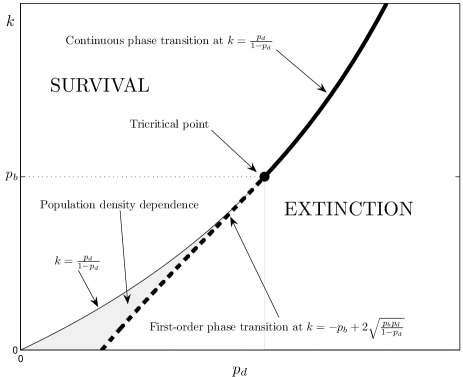
For $k\geq p_{\rm b}$, $\bar{\rho}_{+}\rightarrow 0$ continuously as $p_{\rm d}\rightarrow k/(1+k)$, indicative of a continuous phase transition with critical point

$$p_{\rm{d_{c}}}(k\geq p_{\rm b})=\frac{k}{1+k}.$$ (5)

For $k<p_{\rm b}$, we have a jump in $\bar{\rho}_{\pm}$ from $(p_{\rm b}-k)/2p_{\rm b}$ to zero, this time at the critical point

$$p_{\rm{d_{c}}}(k<p_{\rm b})=\frac{(k+p_{\rm b})^{2}}{4p_{\rm b}+(k+p_{\rm b})^{2}}.$$ (6)

Further, for $k<p_{\rm b}$, we have a region

$$\frac{k}{1+k}\;<\;p_{\rm d}\;\leq\;\frac{(k+p_{\rm b})^{2}}{4p_{\rm b}+(k+p_{\rm b})^{2}}$$ (7)

where the survival of the population is dependent on the population density. In fact, we have extinction for

$$\rho(t)<\bar{\rho}_{-}(k<p_{\rm b},p_{\rm d}).$$ (8)

For $k<p_{\rm b}$ we therefore have a first-order phase transition. The two phase transition lines meet at the point $k=p_{\rm b}$, defining the position of the tricritical point $k^{*}$. At the MF level then, we have a phase diagram as shown in figure 1.

Figure 1: Mean field phase diagram showing the continuous phase transition occurring for $k\geq p_{\rm b}$ and the first-order phase transition for $k<p_{\rm b}$. Equations (5-6) have been re-arranged in the figure to make $k$ the dependent variable.

In the region to the left of the transition lines, there exists at least one real and positive steady state. In the shaded region only, there exist two such steady states with none existing to the right of the transition lines. The tricritical point not only marks the intersection of the first-order and continuous phase lines, but also the line bordering the region with population density dependence.

3 The cluster approximation technique

The MF technique that we employed in the previous section assumed independence between individual sites. In reality there exist, of course, correlations between nearby sites. Increasing improvements to our original MF equation could then be made by considering pairs, triplets, quadruplets and so on, of adjacent sites. Such an approach was developed by ben-Avraham and Köhler, called the $(n,m)$-cluster approximation method [10].

We direct the interested reader to ben-Avraham and Köhler’s paper [10] and others (for example [11, 12] and references therein) for a detailed explanation of the approach. Briefly, the method involves examining clusters of size $n$. For sites $1,2,\dots,j$, we denote $P_{s_{1}s_{2}\dots s_{j}}(t)$ as the probability that the $j$ sites are in state $\{s_{1}s_{2}\dots s_{j}\}$ at time $t$. The method is concerned with how $P_{s_{1}s_{2}\dots s_{n}}(t)$ changes in time and involves deriving a system of master equations for $P_{\{s_{i}\}}(t)$. Since $s_{i}=0$,1 in our case, there are $2^{n}$ such equations. It is, however, easy to see that the number of independent equations is much smaller than this (see, for example, [10]).

Since we are concerned with clusters of size $n$, we need a way to approximate $P_{s_{1}s_{2}\dots s_{n}}$ from clusters of size $N>n$. In their $(n,m)$-approximation, ben-Avraham and Köhler consider adjacent clusters of size $n$ with an overlap of $m<n$ sites. Using the Bayesian extension process, the approximation is then,

$$P_{s_{1}s_{2}\dots s_{N}}=\frac{\prod_{j=0}^{N-n}P_{s_{j+1}\dots s_{j+n}}}{\prod_{j=n-m}^{N-n}P_{s_{j+1}\dots s_{j+m}}}.$$ (9)

For example, the $(3,2)$ approximation for a cluster of size six is given by

$$P_{s_{1}s_{2}s_{3}s_{4}s_{5}s_{6}}=P_{s_{1}s_{2}s_{3}}\frac{P_{s_{2}s_{3}s_{4}}}{P_{s_{2}s_{3}}}\frac{P_{s_{3}s_{4}s_{5}}}{P_{s_{3}s_{4}}}\frac{P_{s_{4}s_{5}s_{6}}}{P_{s_{4}s_{5}}}.$$ (10)

Ben-Avraham and Köhler found that the $(n,n-1)$-approximation yields the most accurate results and is termed the $n$-site approximation for short.

3.1 The 2-site approximation

The simple 1-site approximation is just our original MF equations, so we examine the 2-site approximation. Introducing the subscripts $\bullet$ and $\circ$ for occupied and empty sites respectively, we have two independent variables, chosen to be the particle density $\rho(t)=P_{\bullet}(t)$ and the pair density $c(t)=P_{\bullet\bullet}(t)$. It is then simple to derive the other 2-site probabilities

$$d(t) = P_{\bullet\circ}(t)=\rho(t)-c(t)=P_{\circ\bullet}(t),$$ (11)

$$e(t) = P_{\circ\circ}(t)=1-2\rho(t)+c(t).$$ (12)

To obtain the master equations, we consider the reactions which change the number of occupied sites $n_{\bullet}$ and the number of pairs of sites $n_{\bullet\bullet}$. The reactions are listed in table 1 along with their probabilities of occurring, given the particle configuration. From this table, the master equations for $\rho$ and $c$ are then derived in the usual way.

Reaction			$\Delta n_{\bullet}$	$\Delta n_{\bullet\bullet}$	Probability
$\bullet\bullet\bullet$	$\longrightarrow$	$\bullet\circ\bullet$	$-1$	$-2$	$p_{\rm d}c^{2}/\rho$
$\bullet\bullet\circ$	$\longrightarrow$	$\bullet\circ\circ$	$-1$	$-1$	$p_{\rm d}cd/\rho$	$\times 2$
$\circ\bullet\circ$	$\longrightarrow$	$\circ\circ\circ$	$-1$	$0$	$p_{\rm d}d^{2}/\rho$
$\bullet\bullet\circ\circ$	$\longrightarrow$	$\bullet\circ\bullet\circ$	$0$	$-1$	$\frac{1}{2}(1-p_{\rm d})(1-k)cde/\rho(1-\rho)$	$\times 2$
$\circ\bullet\circ\bullet$	$\longrightarrow$	$\circ\circ\bullet\bullet$	$0$	$+1$	$\frac{1}{2}(1-p_{\rm d})(1-k)d^{3}/\rho(1-\rho)$	$\times 2$
$\bullet\circ\circ$	$\longrightarrow$	$\bullet\bullet\circ$	$+1$	$+1$	$\frac{1}{2}(1-p_{\rm d})kde/(1-\rho)$	$\times 2$
$\bullet\circ\bullet$	$\longrightarrow$	$\bullet\bullet\bullet$	$+1$	$+2$	$\frac{1}{2}(1-p_{\rm d})kd^{2}/(1-\rho)$	$\times 2$
$\bullet\bullet\circ\circ$	$\longrightarrow$	$\bullet\bullet\bullet\circ$	$+1$	$+1$	$\frac{1}{2}(1-p_{\rm d})p_{\rm b}cde/\rho(1-\rho)$	$\times 2$
$\bullet\bullet\circ\bullet$	$\longrightarrow$	$\bullet\bullet\bullet\bullet$	$+1$	$+2$	$\frac{1}{2}(1-p_{\rm d})p_{\rm b}cd^{2}/\rho(1-\rho)$	$\times 2$

Table 1: Reactions for the 2-site approximation where, reactions such as $\bullet\bullet\circ\bullet\longrightarrow\bullet\circ\bullet\bullet$ for which $\Delta n_{\bullet}=\Delta n_{\bullet\bullet}=0$, have been ignored. A symmetry factor arising from the parity symmetry has been included (right column) rather than writing both equations down.

We note that whereas diffusion of the particles did not feature at all in the 1-site approximation, it does appear in the 2-site approximation since $n_{\bullet\bullet}$ can be affected (see rows four and five in table 1).

Deriving the master equations for $\rho$ and $c$, we have

$$\frac{{\rm d}\rho}{{\rm d}t} = (1-p_{\rm d})\frac{(\rho-c)(p_{\rm b}c+k\rho)}{\rho}-p_{\rm d}\rho,$$ (13)

$$\frac{{\rm d}c}{{\rm d}t} = (1-p_{\rm d})\frac{(\rho-c)\left[(1-k)(\rho^{2}-c)+(1-c)(k\rho+p_{\rm b}c)\right]}{\rho(1-\rho)}-2p_{\rm d}c,$$ (14)

where we have used such relations as $d+e=1-\rho$. We notice that, if we make the assumption that all the sites are independent so that $c=\rho^{2}$, we return to our original MF equation. Solving the $\rho$-equation, we have the steady states

$$\bar{\rho}_{0} = 0,$$

$$\bar{\rho}_{\pm} = \frac{c\left[p_{\rm b}-k\pm\sqrt{(p_{\rm b}-k)^{2}-4p_{\rm b}\left(\frac{p_{\rm d}}{1-p_{\rm d}}-k\right)}\right]}{2\left(\frac{p_{\rm d}}{1-p_{\rm d}}-k\right)}.$$ (15)

These roots are very similar to the roots found in the original MF approximation except for the extra prefactor

$$\frac{c}{\left(\frac{p_{\rm d}}{1-p_{\rm d}}-k\right)}.$$ (16)

Similar to before then, so long as $c>0$, for $k<p_{\rm b}$, we have a first order phase transition at

$$p_{\rm d}=\frac{(k+p_{\rm b})^{2}}{4p_{\rm b}+(k+p_{\rm b})^{2}}.$$ (17)

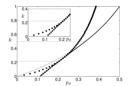
We note that critical point $p_{\rm{d_{c}}}=k/(1+k)$ is no longer valid because of the denominator in the prefactor. To find the critical points then, we solve these equations numerically and plot the results for the 1-site and 2-site approximations in figure 2.

Figure 2: Phase diagram according to the cluster approximation method. The lines show the original MF and the markers the numerically obtained values for the 2-site approximation. The region in between the two lines and between the different markers show the density dependence region. The inset shows the intersection of the two markers for the 2-site approximation showing the tricritical point. The horizontal hashed lines in both plots show the values of $k^{*}$ according to both approximations.

To determine the position of the critical points, for values of $k$ and $p_{\rm d}$, we numerically found all of the real steady states with $0<\bar{c},\bar{\rho}\leq 1$. Counting the number of such steady states indicated which region of the phase diagram we were in. Using an iterative procedure enabled us to locate the boundaries between the regions with zero, one and two such steady states as outlined in the phase diagram in figure 1. For increasing $p_{\rm d}$, the first-order transition lines were indicated by the number of such steady states changing from two to zero and from one to zero for the continuous transition. The tricritical point $k^{*}$ is then given by the intersection of these two lines.

We can further test the stability of the steady states by examining the stability matrix

$$A=\left(\begin{array}[]{cc}\frac{\partial}{\partial\rho}\left(\frac{{\rm d}\rho}{{\rm d}t}\right)&\frac{\partial}{\partial c}\left(\frac{{\rm d}\rho}{{\rm d}t}\right)\\ \frac{\partial}{\partial\rho}\left(\frac{{\rm d}c}{{\rm d}t}\right)&\frac{\partial}{\partial c}\left(\frac{{\rm d}c}{{\rm d}t}\right)\end{array}\right),$$ (18)

evaluated at the steady states. By calculating the eigenvalues of $A$, we have that if both eigenvalues are negative, the steady state is stable, otherwise it is unstable. Testing the non-zero steady states, we find an unstable state in the density dependent region only.

As we see in figure 2, for small values of $k$, the analytical value for the critical points from the 1-site and 2-site approximations are identical. We see, further, that the position of the tricritical point (intersection of the different markers in the figure) is at a lower value of $k$ than the 1-site approximation. Numerically, we found it to be at $k=0.2139$ - less than half of the original MF prediction.

3.2 Higher order approximations

Until now, isolated particles have not been considered appropriately. If we aim to build a more accurate approximation, we need to be able to consider such particles. By examining the 3-site approximation, for example, we consider such probabilities as $P_{\circ\bullet\circ}$. Clearly, the price that we pay is an increase in complexity since the number of variables and equations increase rapidly. We derived equations for higher order approximations for $n\leq 5$. The $n=5$ case required 13 independent variables with over 1,100 reactions having to be considered.

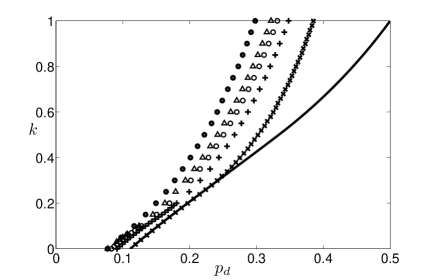
The results for the approximations and simulation results for the critical points are shown in figure 3 a).

a)	b)

Figure 3: a) Numerical results for the critical point for various values of $k$. The line shows the original MF approximation ($n=1$ and the markers (from right to left) the $n=2$, 3, 4 and 5. The circles show the numerical simulation results. c) The approximation for $p_{\rm{d_{c}}}$ for $k=1$ for the different values of $n$. The circle shows the numerical value with the hashed line showing an extrapolation through the points for $n=4$ and $n=5$. The inset shows the tricritical point $k^{*}(n)$ with, again, a hashed line showing an extrapolation.

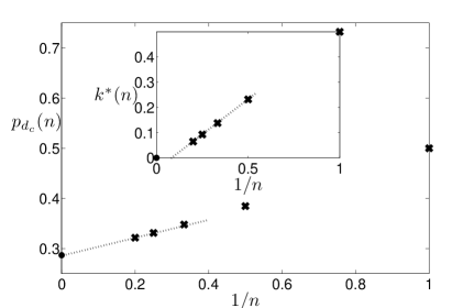
We clearly see how increasing the size of the clusters gives more accurate approximations for the behaviour of the model when comparing to the MC simulation results. In particular, for $k=1$, we show in the main plot of figure 3 b), the approximated values for $p_{\rm{d_{c}}}(n)$ against $1/n$. An extrapolation of the results as $n\rightarrow\infty$ shows excellent agreement with the MC value. Unfortunately, at the first-order phase transition, when the number of real and positive steady state solutions decrease from two to zero, such an extrapolation does not lead to good agreement. This is likely to be due to the fact that at the continuous phase transition, the correlation length is infinite and therefore considering increasingly large numbers of adjacent sites will lead to more accurate approximations. At first-order phase transitions, since the correlation length remains finite, for $n>\xi_{\perp}$ we would expect the approximations for $p_{\rm{d_{c}}}$ to be independent of $n$.

We can further plot the value of the tricritical point as a function of cluster size $n$ and, again, extrapolate. As the inset of figure 3 b) shows, the position of $k^{*}(n)$ decreases with $n$, appearing to become zero for some finite $n$. In other words, for sufficiently large $n$, the corresponding $n$-site cluster approximation would predict no first-order phase transition. This, however, would be surprising since we would expect such behaviour to be true only as $n\rightarrow\infty$. Since the tricritical transition is infinitesimally close to a first-order transition though, we may well expect a tailing-off of this apparent linear behaviour for large $n$.

4 Conclusions

We have seen how, for this model, the analytical cluster-approximation method seems to correctly predict a continuous phase transition in 1+1 dimensions across the whole phase space as $n\rightarrow\infty$. Further, the method predicts, with a high degree of accuracy, the critical point for continuous phase transitions only. These findings highlight the power of the method for this case and will hopefully lead on to further examination of the techniques involved.

References

- [1] Hinrichsen H 2000 cond-mat/0006212
- [2] Dickman R and Tomé T 1991 Phys. Rev. A 44 4833–4838
- [3] Fiore C E and Oliveira M 2004 Phys. Rev. E. 70 046131
- [4] Tomé T and Oliveira M 2001 Phys. Rev. Lett. 86 5643
- [5] Cardozo G and Fontanari J 2006 Eur. Phys. J. B 51 555–561
- [6] Windus A and Jensen H 2008 New J. Phys. 10 113023
- [7] Windus A and Jensen H 2007 J. Phys. A: Math. Theor. 40 2287–2297
- [8] Grassberger P 2006 J. Stat. Mech. - Theory E. P01004
- [9] Lübeck S 2006 J. Stat. Phys. 123 193 – 221
- [10] ben Avraham D and Köhler J 1992 Phys. Rev. A. 45 8358–8370
- [11] Ódor G and Szolnoki A 2005 Phys. Rev. E 71 066128
- [12] Szolnoki A 2002 Phys. Rev. E 66 057102