Quantifiers for randomness of chaotic pseudo random number generators

Abstract

We deal with randomness-quantifiers and concentrate on their ability do discern the hallmark of chaos in time-series used in connection with pseudo random number generators (PRNG). Workers in the field are motivated to use chaotic maps for generating PRNGs because of the simplicity of their implementation. Although there exist very efficient general-purpose benchmarks for testing PRNGs, we feel that the analysis provided here sheds additional didactic light on the importance of the main statistical characteristics of a chaotic map, namely, i) its invariant measure and ii) the mixing constant. This is of help in answering two questions that arise in applications, that is, (1) which is the best PRNG among the available ones? and (2) If a given PRNG turns out not to be good enough and a randomization procedure must still be applied to it, which is the best applicable randomization procedure?. Our answer provides a comparative analysis of several quantifiers advanced in the extant literature.

I Introduction

Chaos theory started more than thirty years ago and changed our world view regarding the role of randomness and determinism. As the statistical characteristics of chaotic systems were better understood Lasota1994 ; Setti2002 ; Beck1997 ; Brown1996 a wide variety of situations emerged in which chaos, instead of stochastic systems, became a “controller of noise” .

Chaos illustrates the rather striking fact that complex behavior arises from simple rules when nonlinearities are present. Since simple chaotic maps are capable to generate stochastic-like signals, implementations based on chaotic systems are usually less involved than those based in more complex algorithms Stojanovski2001 ; Stojanovski2001b ; Kocarev2003 . One tryes to apply this notion to generate PRNGs because random numbers are widely used not only in cryptography and Monte Carlo applications but in less obvious applications Ecuyer1994 ; Pecora1990 ; Kocarev1995 ; Hidalgo2001 ; Fernandez2003 . We mention just a couple of them: 1) in spread spectrum techniques, a binary signal is mixed with a random number sequence to spread the spectrum over a wider frequency range. Using different random number sequences it is possible to share a communication channel among several users Dinan1998 ; Mazzini1997a ; Shan2006 ; DeMicco2007B . Reduction of electromagnetic interference is another important benefit of the spread spectrum effect Setti2000 ; Callegari2002A ; 2) Consider a low frequency signal immersed in a high frequency digital noise. Sampling at time intervals defined by a random number sequence, the resultant signal becomes filtered without using any coil or capacitor that are expensive, specially in power systems Petrocelli2007 .

Truly random numbers are not attainable from computers and it is likely that we will ever be able to get them from “natural” sources, since one commonly assumes that any system is governed by underlying physical rules and consequently it is deterministic. A successful strategy to build up a PRNG is to start with the time series of a simple nonlinear chaotic map and to apply to it an adequate randomizing procedure so as to “heighten/boost” its stochastic nature. Such strategy requires a quantitative evaluation of the improvement achieved after effecting the procedure. In Gonzalez2005 the Statistical Complexity Measure originally proposed by López Ruiz et al. Lopez1995 and later modified by Lamberti et al. Lamberti2004 was used to quantify the effectiveness of such randomizing modus operandi when applied to a Lorenzian chaotic system. It was also shown there that a widely employed course of action -the mixing of two chaotic signals- is not effective in this respect, contrary to what one might expect. In this vein it is important to note that general-purpose tests available in the open literature tests are not designed taking into account the particular characteristics of a chaotic map. Instead, one can appreciate in Rosso2007C the fact that the deterministic nature of chaotic dynamics leaves special manifestations in the associated time series that can be revealed only by recourse to adequate statistical quantifiers.

In Demicco2008 chaotic maps were randomized by means of two different randomizing procedures, namely, discretization and skipping. The idea of concocting an “information” plane, called the entropy-complexity plane, was advanced in order to use it as a means to ascertain the effectiveness of each of these two modus operandis. The main difference of this information plane with other Complexity-Entropy diagrams is the joint use in it of two different probability distribution functions, both associated to the pertinent time series.

Other important tools at our disposal are to be mentioned as well. In a recent and excellent report, Marwan et al. reviewed applications of so-called Recurrence Plots for a wide variety of fields and endeavors. They also proposed several measures to quantify the recurrence plots’ characteristics Marwan2007 . Additionally, two useful information-theoretic quantifiers of randomness, the rate entropy and the Excess Entropy were proposed in Feldman2008 as coordinates of a Complexity-Entropy diagram.

In the present work we explore combinations of all the above mentioned quantifiers with the purpose to answer the following questions: 1) among several chaotic maps, just which is the one that generates the best time series?; 2) which is the best strategy -Discretization or Skipping- to randomize a given chaotic time series?. The ensuing quantifiers-testing will be made by means of two representative chaotic maps (and their iterates).

The paper is organized as follows: the statistical properties of a chaotic map and its iterates is reviewed in section II. Section III describes each of the analyzed quantifiers. Section IV deals with results for two representative maps and, finally, conclusions are presented in Section V.

II Statistical Properties of a Chaotic Map

Let $f$ be a chaotic map on the interval $[0,1]$. Suppose the map has an invariant measure $\mu(x)$. Then the map is ergodic if for any integrable test function $Q(x)$, and for an arbitrary initial condition $x_{0}$ (up to a set of zero $\mu$-measure), the time average is equal to the ensemble average:

$$\overline{Q}=\langle Q\rangle\;.$$ (1)

Equation (1) is a consequence of the famous Birkhoff ergodic theorem Cornfeld1982 . Mixing is an even stronger requirement than ergodicity. A map is called “mixing” if any smooth initial probability density $\rho(x)$ converges to the invariant measure $\mu(x)$ after enough successive iterations. Mixing implies ergodicity. The reverse, however, is not true Beck1990 .

There exists an equivalent definition of mixing via correlation functions. Let $\phi_{1}(x)$ and $\phi_{2}(x)$ be two integrable test-functions and define the generalized correlation function of the map $f$ by

$$C(\phi_{1},\phi_{2},n)=\lim_{J\rightarrow\infty}\frac{1}{J}\sum_{j=0}^{J-1}\phi_{1}(x_{j+n})\phi_{2}(x_{j})-\langle\phi_{1}\rangle\langle\phi_{2}\rangle\;,$$ (2)

where

$$\langle\phi_{i}\rangle=\lim_{J\rightarrow\infty}\frac{1}{J}\sum_{j=0}^{J-1}\phi_{i}(x_{j})\;.$$ (3)

The map is mixing if, for arbitrary $\phi_{1}$ and $\phi_{2}$,

$$\lim_{n\rightarrow\infty}C(\phi_{1},\phi_{2},n)=0\;.$$ (4)

Let us stress that it is not easy to prove that $f$ is a mixing map because the mixing condition given in Eq. (4) must be fulfilled for arbitrary test functions. Formally, every mixing map $f$ has an associated Perron-Frobenius operator $\mathcal{L}$ Beck1990 that determines the time evolution of any initial density $\rho_{0}(x)$ towards the invariant measure $\mu(x)$:

$$\rho_{n+1}=\mathcal{L}[\rho_{n}]\;.$$ (5)

The explicit formal expression for the Perron-Frobenius operator for a one-dimensional map $f$ is given by Beck1990

$$\mathcal{L}[\rho_{y}]=\sum_{x\epsilon f^{-1}(y)}\frac{[\rho_{0}(x)]}{|f^{\prime}(x)|}\;.$$ (6)

This operator $\mathcal{L}$ has a set of eigenfunctions $\psi_{\alpha}(x)$ and eigenvalues $\eta_{\alpha}$. The invariant measure $\mu(x)$ is the eigenfunction corresponding to the largest eigenvalue $\eta_{0}=1$. The full set of eigenfunctions and eigenvalues may be used as a basis to express any density:

$$\rho_{0}(x) = \sum_{\alpha}c_{\alpha}\psi_{\alpha}(x)\ ,$$

$$\rho_{n}(x) = \mathcal{L}^{n}\rho_{0}(x)=\sum_{\alpha}\eta_{\alpha}^{n}c_{\alpha}=c_{0}\psi_{0}(x)+R_{n}\ .$$ (7)

The eigenvalue with the second largest absolute value, $\eta_{1}$, has a ”distinguished” physical meaning: it is related with the mixing constant $r_{mix}$ that governs the relaxation of exponentially mixing maps:

$$|R_{n}|\sim|\eta_{1}|^{n}\sim\exp(-n/r_{mix})\;.$$ (8)

The invariant measure $\mu(x)$ gives the histogram of the time series and the ideal PRNG must have $\mu(x)=const$. The mixing constant $r_{mix}$ gives the transient characteristic time DeMicco2007B ; Petrocelli2007 ; Mazzini1997a ; Rovatti2004a ; Rovatti2004b and its ideal value is $r_{mix}=0$. In many applications of PRNGs both the invariant measure and the mixing constant are relevant.

The analytical expression of the invariant measure $\mu(x)$ of a given map $f$ is usually not known. Exceptions are the logistic map in full chaos, and the piecewise-linear maps. The mixing constant $r_{mix}$ has been analytically obtained only for piecewise-linear maps. For other maps it must be numerically obtained by means of a piecewise linear approximation of the map Lasota1994 ; Beck1997 .

It is then obviously convenient to have quantifiers for measuring the uniformity of the invariant measure $\mu(x)$, and the mixing constant $r_{mix}$, for any chaotic map. These quantifiers are useful to compare time series coming from different chaotic maps and also to assess the improvements produced by randomization procedures.

It is possible to show that the invariant measure of $f^{d}$ is identical to the invariant measure of $f$. Also, the mixing constant $r_{mix}$ for $f^{d}$ is lower that the mixing constant for $f$. The iteration of a map is one of the randomization procedures proposed in the literature, being used to diminish $r_{mix}$. This procedure is also known as Skipping because iterating is tantamount to skipping values in the original time series, which does not change $\mu(x)$ and, consequently, is not conductive to a randomization of chaotic maps with $\mu(x)\neq const$. In this paper we will use “skipping” as a method of quantifier-analysis.

III Quantifiers for the invariant measure and mixing constant

In this section we review several quantifiers proposed for measuring the main statistical properties of chaotic PRNGs. The quantifiers are classified according to their origin into three classes: (1) quantifiers based on Information Theory Lopez1995 ; Rosso2007C ; Lamberti2004 ; (2) quantifiers based on Recurrence Plots Eckmann1987 ; Marwan2007 ; (3) quantifiers based on intrinsic computation Feldman2008 .

III.1 Quantifiers based on Information Theory

They are appropriate functionals of the probability distribution function (PDF). Let $\{x_{i}\}$ be the time series under analysis, with length $M$. There are infinite possibilities to assign a PDF to a given time series, a subject that will be given due consideration below. In the meantime, suppose that the PDF is discrete and is given by $P=\{p_{i};i=\cdots,N\}$. One defines then various quantities, namely,

1. Normalized Shannon Entropy $H[P]$. Let $S[P]$ be the Shannon Entropy

   $$S[P]=-\sum_{i=1}^{N}p_{i}\;\ln({p_{i}})\ .$$ (9)

   Is is well known that the maximum $S_{max}=\ln(N)$ is obtained for $P_{e}=\{1/N,\cdots,1/N\}$, that is, the uniform PDF. A “normalized” entropy $H[P]$ can also be defined in the fashion

   $$H[P]=S[P]/S_{max}\ .$$ (10)

2. Statistical Complexity Measure. A full discussion about Statistical Complexity Measures exceeds the scope of this presentation. For a comparison amongst different complexity measures see the excellent paper by Wackerbauer et al. Wackerbauer1994 . In this paper we adopt the definition by López Ruiz-Mancini-Calbet seminal paper Lopez1995 with the modifications advanced in Lamberti2004 so as to ensure that the concomitant SCM-version becomes (i) able to grasp essential details of the dynamics, (ii) an intensive quantity and, (iii) capable of discerning both among different degrees of periodicity and chaos Rosso2007C . The ensuing measure, to be referred to as the intensive statistical complexity, is a functional $C[P]$ that reads

   $$C[{P}]=Q_{J}[{P,P_{e}}]\cdot H[{P}],$$ (11)

   where $Q_{J}$ is the “disequilibrium”, defined in terms of the so-called extensive Jensen-Shannon divergence (which induces a squared metric) Lamberti2004 . One has

   $$Q_{J}[{P,P_{e}}]=Q_{0}\cdot\{S[(P+P_{e})/2]-S[P]/2-S[P_{e}]/2\},$$ (12)

   with $Q_{0}$ a normalization constant ($0\leq Q_{J}\leq 1$) that reads

   $$Q_{0}=-2\left\{\left(\frac{N+1}{N}\right)\ln(N+1)-2\ln(2N)+\ln N\right\}^{-1}.$$ (13)

   We see that the disequilibrium $Q_{J}$ is an intensive quantity that reflects on the systems’s “architecture”, being different from zero only if there exist “privileged”, or “more likely” states among the accessible ones. $C[P]$ quantifies the presence of correlational structures as well Martin2003 ; Lamberti2004 . The opposite extremes of perfect order and maximal randomness possess no structure to speak of and, as a consequence, $C[P]=0$. In between these two special instances a wide range of possible degrees of physical structure exist, degrees that should be reflected in the features of the underlying probability distribution. In the case of a PRNG the “ideal” values are $H[{P}]=1$ and $C[{P}]=0$.

As pointed out above, $P$ itself is not a uniquely defined object and several approaches have been employed in the literature so as to “extract” $P$ from the given time series. Just to mention some frequently used extraction procedures: a) time series histogram Martin2004 , b) binary symbolic-dynamics Mischaikow1999 , c) Fourier analysis Powell1979 , d) wavelet transform Blanco1998 ; Rosso2001 , e) partition entropies Ebeling2001 , f) permutation entropy Bandt2002a ; Keller2005 , g) discrete entropies Amigo2007B , etc. There is ample liberty to choose among them. In Demicco2008 two probability distribution were proposed as relevant for testing the uniformity of $\mu(x)$ and the mixing constant: (a) a $P$ based on time series’ histograms and (b) a $P$ based on ordinal patterns (permutation ordering) that derives from using the Bandt-Pompe method Bandt2002a .

For extracting $P$ via the histogram divide the interval $[0,1]$ into a finite number $N_{bin}$ of non overlapping subintervals $A_{i}$: $[0,1]=\bigcup_{i=1}^{N_{bin}}A_{i}$ and $A_{i}\bigcap A_{j}=\emptyset~{}\forall i\neq j$. Note that $N$ in eq. (9) is equal to $N_{bin}$. Of course, in this approach the temporal order of the time-series plays no role at all. The quantifiers obtained via the ensuing PDF are called in this paper $H^{(hist)}$ and $C^{(hist)}$. Let us stress that for time series within a finite alphabet it is relevant to consider an optimal value of $N_{bin}$ (see i.e. Demicco2008 ).

In extracting $P$ by recourse to the Bandt-Pompe method the resulting probability distribution $P$ is based on the details of the attractor-reconstruction procedure. Causal information is, consequently, duly incorporated into the construction-process that yields $P$. The quantifiers obtained via the ensuing PDF are called in this paper $H^{(BP)}$ and $C^{(BP)}$. A notable Bandt-Pompe result consists in getting a clear improvement in the quality of information theory-based quantifiers Larrondo2005 ; Larrondo2006 ; Kowalski2007 ; Rosso2007C ; Rosso2007A ; Rosso2007B ; Zunino2007A ; Zunino2007B .

The extracting procedure is as follows. For the time-series $\{x_{t}:t=1,\cdots,M\}$ and an embedding dimension $D>1$, one looks for “ordinal patterns” of order $D$ Bandt2002a ; Keller2003 ; Keller2005 generated by

$$(s)\mapsto\left(x_{s-(D-1)},x_{s-(D-2)},\cdots,x_{s-1},x_{s}\right)\ ,$$ (14)

which assign to each “time $s$” a $D$-dimensional vector of values pertaining to the times $s,s-1,\cdots,s-(D-1)$. Clearly, the greater the $D-$value, the more information on “the past” is incorporated into these vectors. By the “ordinal pattern” related to the time $(s)$ we mean the permutation $\pi=(r_{0},r_{1},\cdots,r_{D-1})$ of $(0,1,\cdots,D-1)$ defined by

$$x_{s-r_{D-1}}\leq x_{s-r_{D-2}}\leq\cdots\leq x_{s-r_{1}}\leq x_{s-r_{0}}.$$ (15)

In order to get a unique result we consider that $r_{i}<r_{i-1}$ if $x_{s-r_{i}}=x_{s-r_{i-1}}$. Thus, for all the $D!$ possible permutations $\pi$ of order $D$, the probability distribution $P=\{p(\pi)\}$ is defined by

$$p(\pi)~{}=~{}\frac{\sharp\{s|s\leq M-D+1;(s)\quad\texttt{has type}~{}\pi\}}{M-D+1}.$$ (16)

In the last expression the symbol $\sharp$ stands for “number”.

The advantages of the Bandt-Pompe method reside in a) its simplicity, b) the associated extremely fast calculation-process, c) its robustness in presence of observational and dynamical noise, and d) its invariance with respect to nonlinear monotonous transformations. The Bandt-Pompe s methodology is not restricted to time series representative of low dimensional dynamical systems but can be applied to any type of time series (regular, chaotic, noisy, or reality based), with a very weak stationary assumption (for $k=D$, the probability for $x_{t}<x_{t+k}$ should not depend on $t$ Bandt2002a ). One also assumes that enough data are available for a correct attractor-reconstruction. Of course, the embedding dimension $D$ plays an important role in the evaluation of the appropriate probability distribution because $D$ determines the number of accessible states $D!$. Also, it conditions the minimum acceptable length $M\gg D!$ of the time series that one needs in order to work with a reliable statistics. In relation to this last point Bandt and Pompe suggest, for practical purposes, to work with $3\leq D\leq 7$ with a time lag $\tau=1$. This is what we do here (in the present work $D=6$ is used).

III.2 Quantifiers based on Recurrence Plots:

Recurrence Plots were introduced by Eckmann et al. Eckmann1987 so as to to visualize the recurrence of states during phase space-evolution. The recurrence plot is a two dimensional representation in which both axes are time-ones. The recurrence of a state appearing at two given times $t_{i},\,t_{j}$ is pictured in the two-dimensional graph by means of either black or white dots, where a black dot signals a recurrence. Of course only periodic continuous systems will have exact recurrences. In any other case one detects only approximate recurrences, up to an error $\epsilon$. The so-called recurrence function can be mathematically expressed as:

$$\mathbf{R}(i,j)=\Theta\left(\varepsilon-\|\overrightarrow{x}(i)-\overrightarrow{x}(j)\|\right),\quad$$ (17)

with $\overrightarrow{x}(i)\in{\Re}^{m}$ and $i,j=1,\cdots,N$. Being $N$ the number of discrete states $\overrightarrow{x}(i)$ considered, $\|\bullet\|$ is a norm, and $\Theta(\bullet)$ is the Heaviside step function.

In the particular case of the PRNGs analyzed in this paper only $1{\mathcal{D}}$ series are considered but the recurrence function-idea can be extended to ${\mathcal{D}}$-dimensional phase spaces or even to suitably reconstructed embedding phase spaces. Of course, the visual impact produced by the recurrence plot is insufficient to compare the quality of different PRNGs, because of the “small scale” structures that may be present in our scenario. Several kind of measures have been defined to quantify these small scale structures Marwan2007 , each measure being a functional of the recurrence function (Eq. (17)). In this paper two kind of Recurrence Plot-measures are considered, namely,

1. Measures based on the recurrence density (measured by the number of points in the Recurrence Plot). In this paper we use the Recurrence Rate ($RR$), given by:

   $$RR(\varepsilon)=\frac{1}{N^{2}}\sum_{i,j=1}^{N}\textbf{R}_{ij}(\varepsilon)\;.$$ (18)

   Note that in the limit $N\rightarrow\infty$, $RR$ is the probability that a state recurs to its $\varepsilon$-neighborhood in phase space. For PRNGs the ideal value would be $RR=0$. But in practice, if no points are to be found in the Recurrence Plot, a larger $\varepsilon$ must be adopted in order that the quantifier may make sense.

2. Diagonal Measures: these are measures related to the histogram $P(\varepsilon,l)$ of diagonal line lengths, given by

   $$P(\varepsilon,l)=\sum_{i,j=1}^{N}\left[1-\textbf{R}_{i-1,j-1}(\varepsilon)\right]\left[1-\textbf{R}_{i+l,j+l}(\varepsilon)\right]\cdot$$

   $$\prod_{k=0}^{l-1}\textbf{R}_{i+k,j+k}(\varepsilon)\;.$$ (19)

   Processes with uncorrelated or weakly correlated behavior originate no (or just very short) diagonals, whereas deterministic processes give rise to “long” diagonals and smaller amount of single, isolated recurrence points. In this paper three measures based on the statistics of diagonal lines are considered:

   1. the deterministic quantifier DET, the ratio of recurrence points that form diagonal structures of at least length $l_{min}$ to all recurrence points

      $$DET=\frac{\sum_{l=l_{min}}^{N}l\cdot P(\varepsilon,l)}{\sum_{l=1}^{N}l\cdot P(\varepsilon,l)}\;;$$ (20)

   2. The average diagonal line length L

      $$L=\frac{\sum_{l=l_{min}}^{N}l\cdot P(\varepsilon,l)}{\sum_{l=l_{min}}^{N}P(\varepsilon,l)}\;;$$ (21)

   3. The entropy $ENTR$ given by

      $$ENTR=-\sum_{l=l_{min}}^{N}P(\varepsilon,l)\ln P(\varepsilon,l)\;.$$ (22)

III.3 Quantifiers based on intrinsic computation

We consider in this paper two quantifiers introduced in Feldman2008 , i.e., the entropy rate $h_{\mu}$ and the entropy excess E. They are defined for time series with a finite alphabet $\mathcal{A}$, which is not a limitation because the $x_{i}$’s may be thought of as real numbers only in analytical studies. In any practical case they are in fact floating point numbers and, consequently, they have only a finite number of allowed $A-$values. A subsequence $s^{L}=\{x_{i},x_{i+1},\cdots,x_{i+L}\}$ is called an $L$-block. Let $P(s^{L})$ denotes the probability of a particular $L$-block. Then the block entropy $H(L)$ is:

$$H(L)\equiv-\sum_{s^{L}}\;P(s^{L})\;log_{2}\,P(s^{L})\ .$$ (23)

The sum runs over all possible blocks of length $L>0$ and $H(0)\equiv 0$ by definition. For stationary processes and sufficiently large $L$, $H(L)\sim L$. On the other hand, the entropy rate $h_{\mu}$ is defined as

$$h_{\mu}(L) = \frac{H(L)}{L}\ ,$$

$$h_{\mu} = \lim_{L\rightarrow\infty}\quad h_{\mu}(L)\ .$$ (24)

The entropy rate is also known as the metric entropy in dynamical systems’ theory and it is equivalent to the thermodynamic entropy density familiar from equilibrium statistical mechanics Feldman2008 . The entropy rate provides a reliable and well understood measure of the randomness or disorder intrinsic to a process. However, this tell us little about the underlying system’s organization, structure or correlations. A measure of system’s organization may be obtained by looking at the manner in which $h_{\mu}(L)$ converges to its asymptotic value $h_{\mu}$. When only observations over length $L$-blocks are taken into account, a process appears to have an entropy rate of $h_{\mu}(L)$ larger than the asymptotic value of $h_{\mu}$. As a result, the process seems to be of a more random nature than it really is by the “excess” amount of $h_{\mu}(L)-h_{\mu}$ bits. Summing these entropy over-estimates over $L$ one obtains the excess entropy Crutchfield1983 :

$$\textbf{E}\equiv\sum_{L=1}^{\infty}\;\left[h_{\mu}(L)-h_{\mu}\right].$$ (25)

III.4 Expected behavior for PRNG

Summing up, the quantifiers to be compared here are: $H^{(hist)}$, $C^{(hist)}$, $H^{(BP)}$, $C^{(BP)}$, $RR$, $DET$, $ENTR$, $L$, $h_{\mu}$, and E. These quantities should tell us how good our PRNG is as compared to the ideal condition $\mu(x)=const$, $r_{mix}=0$. $H^{(hist)}$ is the natural quantifier to measure a non constant $\mu(x)$, with value $1$ for the ideal PRNG. It does not depend on the order of appearance of a given time-series event, but only in the number of times such event takes place. As for $H^{(hist)}$, it is not able to uncover any change in $r_{mix}$-values. Thus, to get a good representation plane we ought to demand a quantifier that changes with $r_{mix}$ and not with $\mu(x)$. To look for such a kind of quantifier we must study $H^{(hist)}$, $C^{(hist)}$, $H^{(BP)}$, $C^{(BP)}$, $RR$, $DET$, $ENTR$, $L$, $h_{\mu}$, and E as functions of $r_{mix}$. A family of iterated maps $f^{d}$ may be used to that end because they share the same invariant measure and $r_{mix}$ is a decreasing function of $d$. The best quantifier for $r_{mix}$ would be that which has maximal variation over the entire family of maps.

IV Application to Logistic Map and Three Way Bernoulli Map

In this Section we present results for the families of iterates of two chaotic well-known maps, the Logistic Map (LOG) and the Three Way Bernoulli Map (TWB), that have been selected, among other possibilities, because they are representative of two different classes of systems.

• LOG is given by:

  $$x_{n+1}~{}=~{}4~{}x_{n}~{}(1-x_{n}),$$ (26)

  and its natural invariant density can be exactly determined, being expressed in the fashion

  $$\rho_{inv}(x)~{}=~{}\frac{1}{\pi\sqrt{x(1-x)}}\;.$$ (27)

  LOG is paradigmatic because it is representative not only of maps with a quadratic maximum, but also emerges when the Lorenz procedure is applied to many continuous attractors with basins that may be approached with the Lorenz method via a $1{\mathcal{D}}$-map (like the Lorenz, Rossler, Colpits ones among others). A non uniform natural invariant density is an important feature in this instance Beck1997 . The ensuing $r_{mix}$-values are also displayed in Table 1. They have been obtained by recourse to the Transfer Operator Method, as described in Beck1997 .

• TWB is given by

  $$x_{n+1}~{}=~{}\left\{\begin{array}[]{ll}3{x_{n}}&\textrm{if $0\leq x_{n}\leq 1/3$}\\ 3{x_{n}}-1&\textrm{if $1/3<x_{n}\leq 2/3$}\\ 3{x_{n}}-2&\textrm{if $2/3<x_{n}\leq 1$}\end{array}\right.\ .$$ (28)

  TWB is representative of the class of piecewise-linear maps as, for example, the Four Way Tailed Shift Map, the Skew Tent Map, the Three Way Tailed Shift Map, etc. All these maps share a uniform natural invariant density Beck1997 . The mixing constant of the whole family of maps $f^{d}$ is given by $r^{d}_{mix}=(1/3)^{d}$ (see table 1).

$d$	TWB	LOG
1	0.56789	0.333333333
2	0.31848	0.111111111
3	0.13290	0.037037037
4	0.05788	0.012345679
5	0.03646	0.004115226
6	0.01791	0.001371742
7	0.01152	0.000457247
8	0.00515	0.000152416

Table 1: $r_{mix}$ as a function of the iteration-order $d$ for LOG and TWB.

For the evaluation of the different quantifiers we used files with $M=50\cdot 10^{6}$ floating point numbers. In the Band-Pompe approach we consider $D=6$ while for histograms we have taken $N_{bin}=2^{16}$. All Recurrence Plots-measures depend on several parameters:

• the dimension $D_{e}$ of the embedding space. In this paper $D_{e}=1$.

• $\varepsilon$, a parameter crucial so as to define just when recurrences occur. We adopted $\varepsilon=1/(2^{16}-1)$ corresponding to $16$-bits numbers.

• $l_{min}$ is the minimum length accepted for diagonal lines. $l_{min}=2$ is used in this paper for all diagonal measures except for $L$ ($l_{min}=1$ is used for $L$).

• $N$ is the number of values used for each realization. In this paper values of $RR$, $DET$, $ENTR$ and $L$ are mean values over $10$ surrogate-series with $N=10000$ data each.

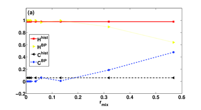
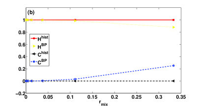
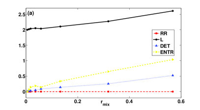
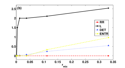
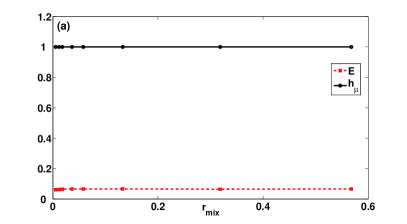
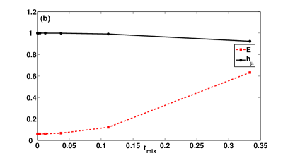
Figures 1, 2, and 3 illustrate the behavior of all the quantifiers for the iterates of LOG (Figs. (a)) and the iterates of TWB (Figs. (b)), respectively. These figures show that the following quantifiers are the ones usable for measuring $r_{mix}$, namely, $C^{(BP)}$, $DET$, $ENTR$, and $L$. On the other hand, the following quantifiers depend on the invariant density but they do not depend on $r_{mix}$: $H^{(hist)}$, $C^{(hist)}$, and $RR$.

Intrinsic computation quantifiers display a completely different behavior for LOG and for TWB. In LOG both quantifiers have no dependence with $r_{mix}$, but in TWB, $h_{\mu}$ decreases as $r_{mix}$ increases while $\mathbf{E}$ is an increasing function of $r_{mix}$. Thus, these parameters do not seem to be convenient ones.

Comparing LOG with TWB by recourse to these parameters shows that TWB is slightly better than LOG. The problem with TWB and with other piecewise linear maps is they are not realistic enough and that their implementation is more involved that for other maps like LOG.

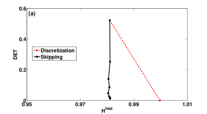
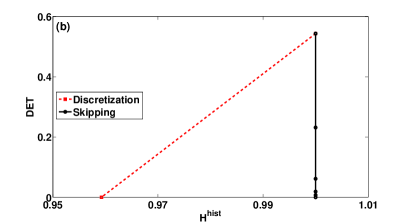
As an application of the above quantifiers we study two usual randomization procedures by means of the representation plane depicted in Fig. 4, employing a quantifier depending on $\mu(x)$ as $x$-axis ($H^{(hist)}$ is selected) and a quantifier depending on $r_{mix}$ as $y$-axis ($DET$ is selected). The first procedure is Skipping and the second one is Discretization (see Demicco2008 ). Skipping has been used as a randomization procedure for piecewise linear maps. The representation plane evidences the fact that this procedure is better than Discretization because these maps already have the ideal invariant measure (they have $H^{(hist)}=1$) and only $r_{mix}$ must be diminished to get the ideal PRNG. Fig. 4 (b) shows that Discretization is a better procedure for LOG because the ideal point $[1,0]$ is not reached by Skipping.

V Conclusions

In summary we were able to show here that:

1. Two classes of quantifiers are required for the evaluation of the quality of a PRNG: a) quantifiers depending on $r_{mix}$ only (and not on $\mu{(x)}$, like $H^{(hist)}$, $C^{(hist)}$, and $RR$ and b) quantifiers depending on $\mu{(x)}$ only (and not on $r_{mix}$), as $C^{(BP)}$, $H^{(BP)}$, $DET$, $L$ and $ENTR$.

2. Intrinsic computation quantifiers are dependent on both $\mu(x)$ and $r_{mix}$ and then they are not convenient for PRNG-analysis with our methodology.

3. Representation planes with one quantifier of each class as coordinate axis allow for different chaotic PRNGs to be compared to each other so as to determine the best one. Furthermore, these representation planes permit one to judiciously select the best randomizing procedure.

Our present results are consistent with those of previous works Gonzalez2005 ; Larrondo2005 ; Demicco2008 .

VI Acknowledgments.

This work was partially supported by the Consejo Nacional de Investigaciones Científicas y Técnicas (CONICET), Argentina (PIP 5569/04, PIP 5687/05, PIP 6036/05), ANPCyT, Argentina (PICT 11-21409/04) and Universidad Nacional de Mar del Plata. OAR gratefully acknowledge support from Australian Research Council (ARC) Centre of Excellence in Bioinformatics, Australia.

Figure 1: Information Theory quantifiers as functions of $r_{mix}$ for: (a) LOG map, (b) TWB map.

Figure 2: Recurrence Plots quantifiers as functions of $r_{mix}$ for: (a) LOG map, (b) TWB map.

Figure 3: Intrinsic Computation quantifiers as functions of $r_{mix}$ for: (a) LOG map, (b) TWB map.

Figure 4: $DET$ as a function of $H^{hist}$, as evaluated in Demicco2008 , for both randomization procedures applied to: (a) LOG map, (b) TWB map.

References

- [1] A. Lasota and M. C. Mackey. Chaos, Fractals, and Noise: Stochastic Aspects of Dynamics. Springer Verlag, 2 edition, 1994.
- [2] G. Setti, G. Mazzini, R. Rovatti, and S. Callegari. Statistical modeling of discrete-time chaotic processes: Basic finite-dimensional tools and applications. Proceedings of the IEEE, 90(5):662–689, Mayo 2002.
- [3] C. Beck and F. Schlögl. Thermodynamics of chaotic systems: an introduction. Cambridge University Press, 1997.
- [4] R. Brown and L.O. Chua. Clarifying chaos: examples and counterexamples. IJBC, 6(2):219–249, Feb 1996.
- [5] T. Stojanovski and L. Kocarev. Chaos-based random number generators - part i: Analysis. IEEE Transactions on Circuits and Systems I: Fundamental Theory and Applications, 48(3):281–288, Marzo 2001.
- [6] T. Stojanovski, J. Pihl, and Kocarev. Chaos-based random number generators - part ii: Practical realization. IEEE Transactions on Circuits and Systems I: Fundamental Theory and Applications, 48(3):382–386, March 2001.
- [7] L. Kocarev and G. Jakimoski. Pseudorandom bits generated by chaotic maps. IEEE Transactions on Circuits and Systems I: Fundamental Theory and Applications, 50(1):123–126, Enero 2003.
- [8] P. L’Ecuyer. Uniform random number generation. Annals of Operations Research, 53:77–120, 1994.
- [9] M. Pecora, L. Carroll, and L. Thomas. Synchronization in chaotic systems. Phys. Rev. Lett., 64(8):821–824, Febrero 1990.
- [10] L. Kocarev and U. Parlitz. General approach for chaotic synchronization with applications to communication. Physical Review Letters, 74(25):5028–5031, 1995.
- [11] R. M. Hidalgo, J. G. Fern ndez, R. R. Rivera, and H. A. Larrondo. Versatile dsp-based chaotic communication system. Electronic Lett., 37:1204–1205, 2001.
- [12] J. G. Fernández, H. A. Larrondo, H. A. Slavin, D. G. Levin, R. M. Hidalgo, and R. R Rivera. Masking properties of apd communication systems. Physica A, 328:351–359, 2003.
- [13] E. H. Dinan and B. Jabbari. Spreading codes for direct sequence cdma and wideband cdma cellular networks. IEEE Communications Magazine, 36(9):48–54, September 1998.
- [14] G. Mazzini, G. Setti, and R. Rovatti. Chaotic complex spreading sequences for aynhchronous ds-cdma-part 1: System modeling and results. IEEE Trans. Circuits Sys. 1, 44(10):937–947, 1997.
- [15] X. Shan, Y. Xia, Y. Ren, and J. Yuan. Spatiotemporal chaotic spreading sequences for cdma communications. In Communication Technology Proceedings, volume 1, pages 530–535, Agosto 2006.
- [16] L. De Micco, C. M. Arizmendi, and H. A. Larrondo. Zipping characterization of chaotic sequences used in spread spectrum communication systems. Institute of Physics Conference Proceedings 913, pages 139–144, 2007.
- [17] G. Setti, M. Balestra, and R. Rovatti. Experimental verification of enhanced electromagnetic compatibility in chaotic fm clock signals. In Proceedings of ISCAS’00, pages III–229–232. IEEE Circuits and Systems Society, 2000.
- [18] S. Callegari, R. Rovatti, and G. Setti. Chaotic modulations can outperform random ones in electromagnetic interference reduction tasks. Electronics Letters, 38(12):543–544, Junio 2002.
- [19] R. A. Petrocelli, L. De Micco, D. O. Carrica, and H. A. Larrondo. Acquisition of low frequency signals immersed in noise by chaotic sampling and fir filters. Proceedings of WISP2007 (IEEE proceedings ISBN 1-4244-0830-X), pages 351–356, 2007.
- [20] C. M. González, H. A. Larrondo, and O. A. Rosso. Statistical complexity measure of pseudorandom bit generators. Physica A, 354:281–300, Agosto 2005.
- [21] R. López-Ruiz, H. L. Mancini, and X. Calbet. A statistical measure of complexity. Phys. Lett. A, 209:321, 1995.
- [22] P. W. Lamberti, M. T. Martín, A. Plastino, and O. A. Rosso. Intensive entropic non-triviality measure. Physica A, 334:119, 2004.
- [23] http://csrc.nist.gov/rng/, http://stat.fsu.edu/pub/diehard/, http://www.iro.umontreal.ca/simardr/random.html.
- [24] O. A. Rosso, H. A. Larrondo, M. T. Martin, A. Plastino, and M. A. Fuentes. Distinguishing noise from chaos. Phys. Rev. Lett., 99:154102–154106, 2007.
- [25] L. De Micco, C. M. González, H. A. Larrondo, M. T. Martin, A. Plastino, and O. A. Rosso. Randomizing nonlinear maps via symbolic dynamics. Physica A, 387:3373–3383, 2008.
- [26] N. Marwan, M. C. Romano, M. Thiel, and J. Kurths. Recurrence plots for the analysis of complex systems. Physics Reports, 438:237–329, 2007.
- [27] D. P. Feldman, C. S. McTague, and P. Crutchfield. The organization of intrinsic omputation: complexity-entropy diagrams and the diversity of natural information processing. arxiv.org:0866.4789[nlin.CD], pages 1–18, junio 2008.
- [28] P. Cornfeld, S. V. Fomin, and Ya. G. Sinai. Ergodic Theory. Springer New York, 1982.
- [29] C. Beck. Ergodic properties of a kicked damped particle. Commun. Math Phys., 130(51), 1990.
- [30] R. Rovatti, G. Mazzini, and G. Setti. On the ultimate limits of chaos-based asynchronous ds-cdma- i: Basic definitions and results. IEEE Transactions on Circuits and Systems I: Fundamental Theory and Applications, 51(7):1336–1347, Julio 2004.
- [31] R. Rovatti, G. Mazzini, and G. Setti. On the ultimate limits of chaos-based asynchronous ds-cdma-ii: Analytical results and asymptotics. IEEE Transactions on Circuits and Systems I: Fundamental Theory and Applications, 51(7):1348–1364, Julio 2004.
- [32] J. Eckmann, S. Oliffson Kamphorst, and D. Ruelle. Recurrence plots of dynamical systems. Europhys. Lett., 4:973–977, 1987.
- [33] R. Wackerbauer, A. Witt, H. Atmanspacher, J. Kurths, and H. Scheingraber. A comparative classification of complexity measures. Chaos, Solitons, Fractals, 4:133–173, 1994.
- [34] M. T. Martín, A. Plastino, and O. A. Rosso. Statistical complexity and disequilibrium. Phys. Lett. A, 311:126–132, 2003.
- [35] M. T. Martin. Ph.D. Thesis, Department of Mathematics,. PhD thesis, Faculty of Sciences, University of La Plata, 2004.
- [36] K. Mischaikow, M. Mrozek, J. Reiss, and A. Szymczak. Construction of symbolic dynamics from experimental time series. Phys. Rev. Lett., 82:1144, 1999.
- [37] G. E. Powell and I. C. Percival. A spectral entropy method for distinguishing regular and irregular motion of hamiltonian systems. J. Phys. A: Math. Gen., 12:2053–2071, 1979.
- [38] S. Blanco, A. Figliola, R. Quian Quiroga, O. A. Rosso, and E. Serrano. Time-frequency analysis of electroencephalogram series (iii): Wavelet packets and information cost function. Phys. Rev. E, 57:932–940., 1998.
- [39] O. A. Rosso, S. Blanco, J. Jordanova, V. Kolev, A. Figliola, M. Schurmann, and E. Başar. Wavelet entropy: a new tool for analysis of short duration brain electrical signals. Journal of Neuroscience Methods, 105:65–75, 2001.
- [40] W. Ebeling and R. Steuer. Partition-based entropies of deterministic and stochastic maps. Stochastics and Dynamics, 1(1):1–17, 2001.
- [41] C. Bandt and B. Pompe. Permutation entropy: a natural complexity measure for time series. Phys. Rev. Lett., 88:174102–1, 2002.
- [42] K. Keller and M. Sinn. Ordinal analysis of time series. Physica A, 356:114–120, 2005.
- [43] J. M. Amigó, L. Kocarev, and I. Tomovski. Discrete entropy. Physica D, 228:77–85, 2007.
- [44] H. A. Larrondo, C. M. González, M. T. Martin, A. Plastino, and O. A. Rosso. Intensive statistical complexity measure of pseudorandom number generators. Physica A, 356:133–138, 2005.
- [45] H. A. Larrondo, M. T. Martin, C.M. González, A. Plastino, and O. A. Rosso. Random number generators and causality. Phys. Lett. A, 352((4- 5)):421–425, Abril 2006.
- [46] A. M. Kowalski, M. T. Martín, A. Plastino, and O. A. Rosso. Bandt-pompe approach to the classical-quantum transition. Physica D, 233:21–31, 2007.
- [47] O. A. Rosso, R. Vicente, and C. R. Mirasso. Encryption test of pseudo-aleatory messages embedded on chaotic laser signals: An information theory approach. Phys. Lett. A, 372:1018–1023, 2008.
- [48] O. A. Rosso, L. Zunino, D. G. Pérez, A. Figliola, H. A. Larrondo, M. Garavaglia, M. T. Martín, and Plastino A. Extracting features of gaussian self—similar stochastic processes via the bandt and pompe approach. Phys. Rev. E, 76(6):061114, 2007.
- [49] L. Zunino, D.G. Pérez, M. T. Martín, A. Plastino, M. Garavaglia, and O. A. Rosso. Characterization of gaussian self-similar stochastic processes using wavelet-based informational tools. Phys. Rev. E, 75:031115, 2007.
- [50] L. Zunino, D.G. Pérez, M. T. Martín, M. Garavaglia, A. Plastino, and O. A. Rosso. Permutation entropy of fractional brownian motion and fractional gaussian noise. Phys. Lett. A, 372:4768–4774, 2008.
- [51] K. Keller and H. Lauffer. Symbolic analysis of high-dimensional time series. Int. J. Bifurcation and Chaos, 13:2657–2668, 2003.
- [52] J. P. Crutchfield and N. H. Packard. Symbolic dynamics of noisy chaos. Physica D, 7:201–223, 1983.