CERN-PH-TH/2008-238, LAPTH-1294/08
Cosmological constraints on a light non-thermal sterile neutrino
Mario A. Acero(a,b,c), Julien Lesgourgues(d,e)
Dipartimento di Fisica Teorica,
Università di Torino,
Via P. Giuria 1, I–10125 Torino, Italy
INFN, Sezione di Torino,
Via P. Giuria 1, I–10125 Torino, Italy
Laboratoire d’Annecy-le-Vieux de Physique Thórique LAPTH,
Université de Savoie, CNRS/IN2P3, 74941 Annecy-le-vieux, France
PH-TH, CERN - CH-1211 Geneva 23, Switzerland
SB-ITP-LPPC, BSP 312 - EPFL, CH-1015 Lausanne, Switzerland
Abstract
Although the MiniBooNE experiment has severely restricted the possible existence of light sterile neutrinos, a few anomalies persist in oscillation data, and the possibility of extra light species contributing as a subdominant hot (or warm) component is still interesting. In many models, this species would be in thermal equilibrium in the early universe and share the same temperature as active neutrinos, but this is not necessarily the case. In this work, we fit up-to-date cosmological data with an extended CDM model, including light relics with a mass typically in the range 0.1–10 eV. We provide, first, some nearly model-independent constraints on their current density and velocity dispersion, and second, some constraints on their mass, assuming that they consist either in early decoupled thermal relics, or in non-resonantly produced sterile neutrinos. Our results can be used for constraining most particle-physics-motivated models with three active neutrinos and one extra light species. For instance, we find that at the confidence level, a sterile neutrino with mass eV can be accommodated with the data provided that it is thermally distributed with , or non-resonantly produced with . The bounds become dramatically tighter when the mass increases. For eV and at the same confidence level, the data is still compatible with a standard thermalized neutrino.
1 Introduction
Neutrino oscillation is a well studied phenomenon, confirmed by strong experimental evidences. Most experimental results are well explained with a three-neutrino oscillation model, involving two independent and well-measured square-mass differences: eV2 [1] and eV2 [2]. However, some other experiments have shown some anomalies which do not fit in this hypothesis (LSND [3], Gallium experiments [4], MiniBooNE low energy anomaly [5]). These anomalous results might be due to unknown systematic effects, but all attempts to identify such systematics have failed until now. Otherwise, they could be interpreted as exotic neutrino physics.
In Ref. [6], the MiniBooNE anomaly was explained through a renormalization of the absolute neutrino flux and a simultaneous disappearance of electron neutrinos oscillating into sterile neutrinos (with ). The LSND and Gallium radioactive source experiment [7, 8, 9] anomalies have been studied in Ref. [10], where is it claimed that all these anomalies could be interpreted as an indication of the presence of, at least, one sterile neutrino with rather large mass (few eV’s). Ref. [11] also studied the compatibility of the Gallium results with the Bugey [12] and Chooz [13] reactor experimental data, concluding that such a sterile neutrino should have a mass between one and two eV’s. Finally, the MiniBooNE collaboration performed global fits of MiniBooNE, LSND, KARMEN2, and Bugey experiments in presence of a fourth sterile neutrino [14] (assuming no renormalization issue for MiniBooNe unlike Ref. [6]). When all four experiments are combined, the compatibility between them is found to be very low (4%); however, when only three of them are included, the compatibility level is usually reasonable (the largest tension being found between LSND and Bugey). In this analysis, the preferred value of the sterile neutrino is usually smaller than 1eV, but still of possible cosmological relevance (for instance, for all four experiments, the best fit corresponds to eV2).
These various developments suggest that it is important to scrutinize cosmological bounds on scenarios with one light sterile neutrino, which could help ruling them out, given that current bounds on the total neutrino mass assuming just three active neutrinos are as low as eV (using WMAP5, BAO and SN data [15]). This result cannot be readily applied to the models which we consider here. Indeed, scenarios with extra neutrinos require a specific cosmological analysis, for the simple reason that besides affecting the total neutrino mass, additional neutrinos also increase the abundance of relativistic particles in the early universe.
From the point of view of Cosmology, there have been many works constraining simultaneously the sum of neutrino masses and the contribution to the relativistic energy density component of the Universe, parametrized as the effective number of neutrinos, (see for example [16, 17, 18, 19, 20, 21]). Most of these works assume either that the heaviest neutrino (and hence the most relevant one from the point of view of free-streaming) has a thermal distribution, sharing the same value of temperature as active neutrinos, or that all neutrinos are degenerate in mass. However, the results of Refs. [22, 23] can also be applied to the case of very light active neutrinos plus one heavier, non-necessarily thermal sterile neutrino, which is the most interesting case for explaining oscillation anomalies. In terms of physical motivations, it is very likely that the light sterile neutrino required by the LSND anomaly acquires a thermal distribution in the early universe, through oscillations with active neutrinos in presence of a large mixing angle [24]. On the other hand, there are some proposals to avoid these contrains (for a list of some scenarios, see [25]). One of such possibilities is based on a low reheating temperature () Universe [26, 27, 28, 29], in which, for a sufficiently low , the sterile neutrinos could be non-thermal [30] and its production would be suppressed [28], such that usual cosmological bounds are evaded. In fact, in these models, sterile neutrinos are allowed to have a large mass without entering in conflict with other experimental results, while MeV ( being the temperature of the cosmic plasma at neutrino decoupling).
In absence of thermalization, cosmological bounds on the sterile neutrino mass become potentially weaker. Hence, it is interesting to study the compatibility of recently proposed scenarios with a light sterile neutrino with the most recent cosmological data, keeping in mind the possibility of a non-thermal distribution. The goal of this paper is hence to study the compatibility of cosmological experimental data (WMAP5 plus small-scale CMB data, SDSS LRG data, SNIa data from SNLS and conservative Lya data from VHS) with the hypothesis of a sterile neutrino with the characteristics sketched above, i.e., with a mass roughly of the order of the electron-Volt, and a contribution to smaller than one.
2 Light sterile neutrino in cosmology: physical effects and parametrization
If a population of free-streaming particles becomes non-relativistic after photon decoupling, its physical effects on the cosmological background and perturbation evolution are mainly described by three quantities:
-
1.
its contribution to the relativistic density before photon decoupling, which affects the redshift of radiation/matter equality, usually parametrized by an effective neutrino number (standing for the relativistic density of the species divided by that of one massless neutrino family in the instantaneous decoupling (id) limit):
(1) with ,
-
2.
its current energy density, which affects (i) the current energy budget of the Universe (with various consequences for the CMB and LSS spectra, depending on which other parameters are kept fixed), and (ii) the amplitude reduction in the small-scale matter power spectrum due to these extra massive free-streaming particles, parametrized by the dimensionless number :
(2) where is the critical density today and the reduced Hubble parameter,
-
3.
the comoving free-streaming length of these particles when they become non-relativistic, which controls the scale at which the suppression of small-scale matter fluctuations occurs. This length can easily be related to the average velocity of the particles today, 111The minimum comoving free-streaming wavenumber is controlled by and by the ratio evaluated when , i.e. when . Given that , the minimum comoving free-streaming length just depends on and ..
However, for whatever assumption concerning the phase-space distribution function , the three numbers (, , ) satisfy a constraint equation. Indeed, the average velocity of the particles today (assumed to be in the non-relativistic regime) is given exactly by
| (3) |
in units where , and taking K. Hence, the three physical effects described above depend on only two independent parameters.
Reducing the physical impact of any population of massive free-streaming particles to these three effects (and two independent parameters) is a simplification: two models based on different non-thermal phase-space distributions can in principle share the same numbers (, , ) and impact the matter power spectrum differently. Indeed, the free-streaming effect depends on the details of (including high statistical momenta like , etc.) However, the conclusions of Ref. [18] indicate that for many models with non-thermal distorsions, observable effects can indeed be parametrized by two combinations of (, , ) with good accuracy: other independent parameters would be very difficult to observe222This conclusion does not apply when the non-thermal distribution has a sharp peak close to . In this case, particles with very small momentum should be counted within the CDM component, not within the extra massive free-streaming component. Otherwise, one would obtain values of and based on an averages between cold and hot/warm particles; then, these parameters would not capture the correct physical effects (see [31]).
Let us compute the three parameters (, , ) for simple cases. For one species of thermalized free-streaming particles with mass , sharing the same temperature as active neutrinos in the instantaneous decoupling limit, one gets:
| (4) |
For a light thermal relic with a Fermi-Dirac distribution and a different temperature , these quantities become
| (5) |
For a non-thermal relic with a free function , there is an infinity of possible models. A popular one is the Dodelson-Widrow scenario [32] (also referred as the “non-resonant production scenario”), motivated by early active-sterile neutrino oscillations in the limit of small mixing angle and zero leptonic asymmetry, which corresponds to the phase-space distribution
| (6) |
where is an arbitrary normalization factor. In this case, in the approximation , the three “observable” parameters read
| (7) |
Hence, a Dodelson-Widrow (DW) model shares that same “observable” parameters (, , ) as a thermal model with and . Actually, for these two models, the degeneracy is exact: it can be shown by a change of variable in the background and linear perturbation equations that the two models are strictly equivalent from the point of view of cosmological observables [33, 18]. As mentioned before, in the general case, two models sharing the same (, , ) are not always strictly equivalent, but can be thought to be hardly distinguishable even with future cosmological data. For instance, the low-temperature reheating model analyzed in [27, 28] leads to a distribution of the form
| (8) |
This model would in principle deserve a specific analysis, but in good approximation we can expect that by only exploring the parameter space of thermal models (or equivalently, of DW models), we will obtain some very generic results, covering in good approximation most possibilities for the non-thermal distorsions.
3 Analysis
3.1 Data
In the following sections, we will present the results of various runs based on the Boltzmann code CAMB [34] and cosmological parameter extraction code CosmoMC [35]. We modified CAMB in order to implement the proper phase-space distribution of the thermal or DW model. For simplicity, we assumed in all runs that the three active neutrinos can be described as massless particles. In order to obtain a Bayesian probability distribution for each cosmological parameters, we ran CosmoMC with flat priors on the usual set of six parameters , , , , , (see e.g. [36]), plus two extra parameters describing the sterile neutrino sector, that will be described in the next sections. We choose the following data set: WMAP5 [37] plus small-scale CMB data (ACBAR [38], CBI [39], Boomerang [40]), the galaxy power spectrum of the SDSS LRG [41] with flat prior on [42, 43], SNIa data from SNLS [44] and conservative Lyman- data from VHS [45]. We do not include more recent Lyman- data sets, which have much smaller errorbars, but for which the deconvolution of non-linear effects depends on each particular cosmological model, and requires specific hydrodynamical simulations.
3.2 General analysis
Our first goal is to obtain simple results with a wide range of applications. Hence, we should not parametrize the effect of sterile neutrinos with e.g. their mass or temperature: in that case, our results would strongly depend on underlying assumptions for . It is clear from section 2 that nearly “universal” results can be obtained by employing two combinations of the “observable parameters” , and (and eventually of other parameters of the CDM model). Here we choose to vary the current dark matter density fraction and the current velocity dispersion . As will be clear from our results, these two parameters capture the dominant observable effects, and lead to very clear bounds, since their correlation with other CDM model parameters is insignificant. Our limits on and apply exactly to the thermal case and DW case, and approximately to most other cases (modulo the caveat described in the second footnote of section 2).
Our parameter space is represented in Figure 1. We adopt a logarithmic scale for and display the interesting range
| (9) |
Indeed, with out dataset, particles with smaller velocities would be indistinguishable from cold dark matter; instead, particles with larger velocities would either have (a case beyond the motivations of this work, and anyway very constrained by the data) or (being indistinguishable from extra relativistic degrees of freedom). Assuming a particular value for and for , it is possible to compute the velocity dispersion as a function of . Since the CMB and LSS data give precise constraints on , regions of equal correspond to thin bands in the (, ) plane. We show these bands in Figure 1 for under the assumption that , which corresponds roughly to the 95% confidence limits (C.L.) from all our runs. These iso- bands are completely model-independent.
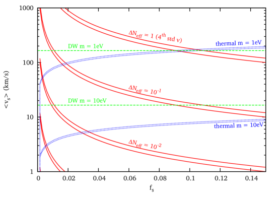
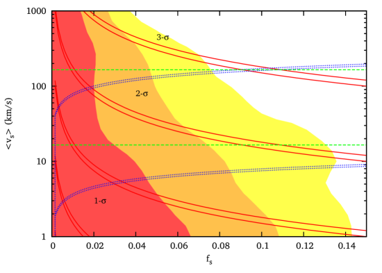
Instead, regions of equal mass can only be plotted for a particular model. In Figure 1, we show the bands corresponding to 1 eV and 10 eV, either in the case of early decoupled thermal relics (blue/dotted lines) or in the DW case (green/dashed lines). For any given mass, these bands intersect each other in a location corresponding to the case of one fourth standard neutrino species with .
We ran CosmoMC with top-hat priors on (in the physical range ) and on (in the range motivated by the previous discussion). Our results are summarized in Figure 1 (bottom). We see that the upper bound on decreases smoothly as the velocity dispersion increases: when the particles have a larger velocity dispersion, their free-streaming wavelength is larger, so the step-like suppression in the power spectrum (which amplitude depends on ) is more constrained. For , we find at the C.L., while for , we find at the C.L. When the velocity dispersion becomes larger than , the upper bound on decreases even faster as a function of . This is the case of a HDM component with significant contribution to the number of relativistic d.o.f., for which the observational bounds derive from a combination of the first and second effects described in section 2: in this limit, in addition to being sensitive to the free-streaming effect, the data disfavor a significant increase of the total radiation density corresponding to of order one or larger.
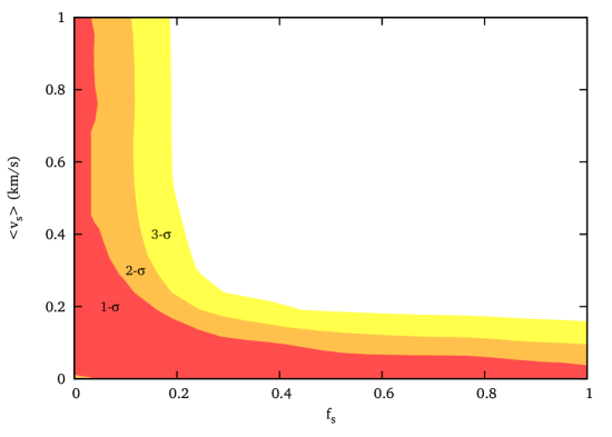
We should stress that the details of our results depend on the underlying priors. For instance, one could use a flat prior on instead of its logarithm. Running in the range with such a prior would give more focus on the large- allowed region of Figure 1. However, it would be more interesting to focus on small velocities, in order to understand how our results can be extended without any discontinuity to the case of warmer and heavier dark matter. For this purpose, we ran CosmoMC with a top-hat prior on , and obtained the results shown in Figure 2. These results are identical to those published in Reference [46] (figure 7). By gluing figure 1 on top of 2, one can obtain a full coverage of the parameter space of CDM models completed by one extra (hot or warm) dark matter species. Figure 2 shows the transition from the region in which this extra species is indistinguishable from cold dark matter (when , the fraction is unconstrained) to the region in which it is warm (for , there is a nearly constant bound at the 2- level). Figure 1 shows instead the transition from warm particles to hot particles (with velocities comparable to those of active neutrinos). The two plots perfectly match each other along the axis, on which the sterile neutrino fraction is bounded by (2-).
3.3 Mass/temperature bounds in the thermal case
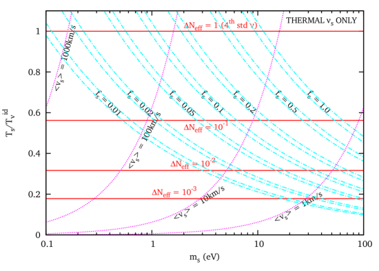
We now focus on the particular case of early decoupled thermal relics, with a Fermi-Dirac distribution and a temperature . These models can be parametrized by the mass and the temperature in units of the neutrino temperature, . Our parameter space – and the correspondence with the previous parameters , , – is shown in Figure 3. In this analysis, we want to focus again on light sterile neutrinos rather than WDM; hence we are not interested in velocities smaller than 1 km/s today. We are not interested either in the case of enhanced particles with . Then, as can be checked in Figure 3, the ensemble of interesting models can be covered by taking a top-hat prior on in the range , and on in the range .
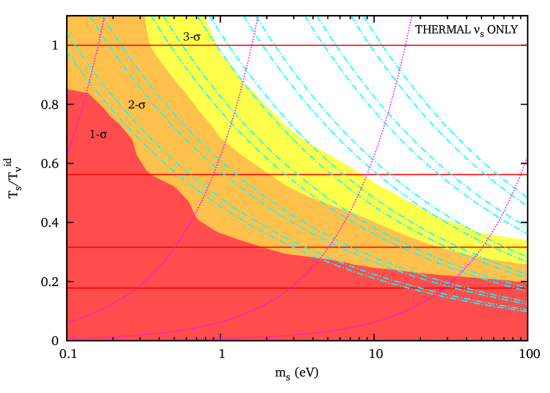
The likelihood contours obtained for this case are shown in Figure 3 (bottom). They are consistent with our previous results: when (and hence ), the upper bound on the sterile neutrino fraction is at the C.L.; then this bound decreases smoothly when increases. For a fourth standard neutrino with , the C.L. (resp. C.L.) bound is eV (resp. 0.9 eV).
This figure can be conveniently used for model building: for a given value of the mass, it shows what should be the maximal temperature of the thermal relics in order to cope with cosmological observations; knowing this information and assuming a particular extension of the particle physics standard model, one can derive limits on the decoupling time of the particle. For instance, for a mass of eV one gets ; for eV, ; while for eV, . This figure can also be applied to thermally produced axions, like in Refs. [47, 48].
3.4 Mass bounds in the DW case
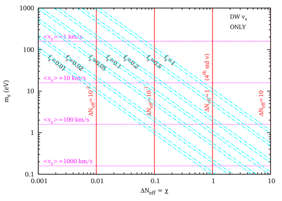
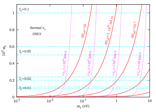
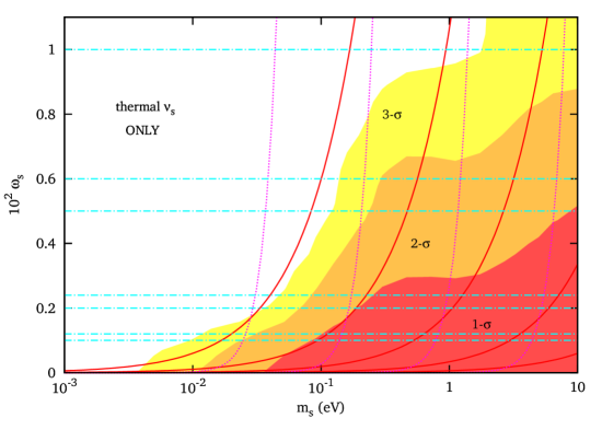
Finally, for Dodelson-Widrow relics with a distribution function equal to that of standard neutrinos suppressed by a factor (which is equal by definition to ), we can parametrize the ensemble of models by and . Our parameter space – and the correspondence with , – is shown in Figure 4. Like in the previous section, we are not interested in a current velocity dispersion smaller than 1 km/s today. Then, as can be checked in Figure 4, the ensemble of interesting models can be covered by taking a top-hat prior on in the range ; in this range, values of smaller than would correspond to tiny values of , i.e. to particles indistinguishable from massless particles; so, we can take a flat prior on in the range .
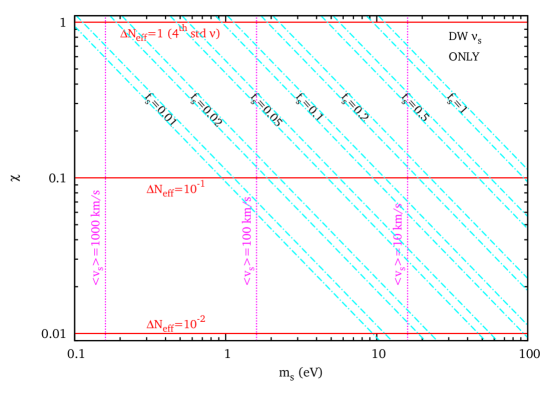
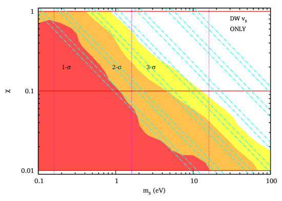
The likelihood contours obtained for this case are shown in Figure 4 (bottom). We are not surprised to find once more an allowed region corresponding to at the C.L. when is negligible with respect to one, or less when grows closer to one. For a fourth standard neutrino with , the two definitions of the mass (following from the thermal or from the DW cases) are equivalent, and indeed we find eV ( C.L.) or eV ( C.L.) like in section 3.3.
This figure can also be useful for model building: for a given value of the mass, it shows what should be the maximal value of compatible with cosmological observations; in turn, this information can be used to put bounds on the mixing angle between this relic and active neutrinos in non-resonant production models à la Dodelson & Widrow. For instance, for a mass of eV, the C.L. gives ; for eV, we get ; while for eV, we get .
3.5 Comparison with previous work
The ensemble of cosmological models that we are exploring here is not different from that studied by Dodelson, Melchiorri & Slosar [23] (called later DMS) or by Cirelli & Strumia [22] (called later CS); the difference between these works and the present analysis consists in a different choice of parameters, priors, data set, and also methodology in the case of CS.
For instance, Figure 6a of CS presents constrains in the space (, ) assuming a DW scenario. Hence, their parameter space is identical to the one we used in section 3.4, excepted for the prior range (which is wider in their case). As far as the data set is concerned, CS use some CMB and galaxy spectrum measurements which are slightly obsolete by now; on the other hand, they employ some additional information derived from BAO experiments, and use SDSS Lyman- data points that we conservatively excluded from this analysis, since they assume a CDM cosmology. Finally, CS performed a frequentist analysis, and their bounds are obtained by minimizing the over extra parameters (while in the present Bayesian analysis, we marginalize over them given the priors).
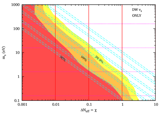
In order to compare our results with CS, we performed a run with top-hat priors on in the range , and on in the range . In this particular run we compute the 90%, 99% and 99.9% C.L., following CS. Our results are shown in Figure 5, and are consistent with those of our general analysis.
In spite of the different data set and methodology, the 90% and 99% contours are found to be in very good agreement with CS in most of the parameter space. The major difference lies in the small mass region, for which CS get more conservative limits on than we do, and find a preference for non-zero values of the effective neutrino number (at the 90% C.L.). This qualitative behavior has been nicely explained in Refs. [42, 43]. It is due to the non-linear corrections applied to the theoretical linear power spectrum before comparing it with the observed SDSS and 2dF galaxy power spectra. The approach used in this work (and in the default version of CosmoMC) consists in marginalizing over a nuisance parameter (describing the scale-dependence of the bias) with a flat prior. Instead, following Ref. [49], CS impose a gaussian prior on . This results in biasing the results towards larger values of , and finding marginal evidence for . Of course, this assumption might turn out to be correct; however, it is argued in Refs. [42, 43] that our knowledge on (based essentially on N-body simulations for some particular cosmological models) is still too uncertain for getting definite predictions.
The analysis of DMS is Bayesian, like ours. The authors use top-hat priors on the two parameters and , roughly the same data set as CS, and employ the distribution function of early decoupled thermal relics. Our results based on the same priors (but a different data set) are shown in Figure 6, and are consistent with the previous sections: at the 2 level, is such that for ; then, the bound on (and therefore on ) decreases smoothly when decreases (and therefore increases). These results differ significantly from those of DMS, who find that the upper bound on peaks near eV and then decreases quickly. We do not observe such a behavior: our upper bound on increases (not so smoothly, but still monotonically) when increases, in agreement with all previous results in this paper. This difference is most likely due to the use made by DMS of more aggressive Lyman- data from SDSS, of different galaxy power spectrum data, and of a prior on , as in CS. This data set puts stronger limits on a possible suppression of the small scale power spectrum. Actually, in absence of sterile neutrinos, the same combination of data is known to produce very strong bounds on neutrino masses, and to prefer slightly larger than one [49]; in presence of light sterile neutrinos, the results of DMS show that this data also imposes a strong bound for , due to its sensitivity to the sterile neutrino free-streaming effect. Our large scale structure data set (conservative Lyman- data from VHS, SDSS-LRG and flat prior on ) is not able to exclude this region.
4 Conclusions
In this work, we studied the compatibility of cosmological experimental data with the hypothesis of a non-thermal sterile neutrino with a mass in the range eV (or more), and a contribution to smaller than one. We computed Bayesian confidence limits on different sets of parameters, adapted to the case of thermal relics (section 3.3), of non-resonantly produced sterile neutrinos à la Dodelson & Widrow (DW, section 3.4), or of generic parameters leading to nearly model-independent results (section 3.2). In each case, we performed a specific parameter extraction from scratch, in order to obtain reliable results assuming flat priors on the displayed parameters. For simplicity, we assumed that the masses of the three active neutrinos are negligible with respect to that of the sterile neutrino.
For a cosmological data set consisting in recent CMB and LSS data, as well as older but very conservative Lyman- data, we found the conditional probability e.g. on the mass of a thermal relic given its temperature, or on the mass of a DW neutrino given its density suppression factor, etc. These proabilities are such that if the fourth neutrino is a standard one (with ), it should have a mass eV ( C.L.) or eV ( C.L.).
At the C.L., a mass eV can be accommodated with the data provided that this neutrino is thermally distributed with , or non-resonantly produced with . The bounds become dramatically tighter when the mass increases. At the same confidence level, a mass of just eV requires either or , while a mass eV requires or .
Our bounds can hopefully be used for constraining particle-physics-motivated models with three active and one sterile neutrinos, as those investigated recently in order to explain possible anomalies in neutrino oscillation data. Many of these models can be immediately localized in our figures 3 or 4. For sterile neutrinos or other particles which do not fall in the thermal or DW category, a good approximation consists in computing their velocity dispersion and localizing the model in our figure 5 333However, this approximation could be not so good when the distribution of the non-thermal relic peaks near , as if part of these relics were actually cold, see [31].. Future neutrino oscillation experiments are expected to test the self-consistency of the standard three-neutrino scenario with increasing accuracy. If anomalies and indications for sterile neutrinos tend to persist, it will be particularly useful to perform joint analysis of oscillation and cosmological data, using the lines of this work for the latter part.
Acknowledgments
M.A.A. would like to thank the International Doctorate on AstroParticle Physics (IDAPP) for financial support, as well as LAPTH for hospitality during the realization of most of this work. M.A.A. and J.L. thank INFN for supporting a visit to the Galileo Galilei Institute for Theoretical Physics, in which this project was initiated. J.L. also acknowledges the support of the EU 6th Framework Marie Curie Research and Training network “UniverseNet” (MRTN-CT-2006-035863). Numerical simulations were performed on the MUST cluster at LAPP, Annecy (IN2P3/CNRS and Université de Savoie).
References
- [1] S. Abe et al., Phys. Rev. Lett. 100, 221803 (2008), arXiv:0801.4589.
- [2] P. Adamson et al., Phys. Rev. D77, 072002 (2008), arXiv:0711.0769.
- [3] A. Aguilar et al., Phys. Rev. D64, 112007 (2001), arXiv:hep-ex/0104049.
- [4] J. N. Abdurashitov et al., Phys. Rev. C73, 045805 (2006), arXiv:nucl-ex/0512041.
- [5] A. A. Aguilar-Arevalo et al., Phys. Rev. Lett. 98, 231801 (2007), arXiv:0704.1500.
- [6] C. Giunti and M. Laveder, Phys. Rev. D77, 093002 (2008), arXiv:0707.4593.
- [7] W. Hampel et al., Phys. Lett. B420, 114 (1998).
- [8] J. N. Abdurashitov et al., Phys. Rev. C59, 2246 (1999), arXiv:hep-ph/9803418.
- [9] J. N. Abdurashitov et al., Astropart. Phys. 25, 349 (2006), arXiv:nucl-ex/0509031.
- [10] C. Giunti and M. Laveder, Mod. Phys. Lett. A22, 2499 (2007), arXiv:hep-ph/0610352.
- [11] M. A. Acero, C. Giunti, and M. Laveder, Physical Review D –, (2008), arXiv:0711.4222.
- [12] Y. Declais et al., Nucl. Phys. B434, 503 (1995).
- [13] M. Apollonio et al., Eur. Phys. J. C27, 331 (2003), arXiv:hep-ex/0301017.
- [14] A. A. Aguilar-Arevalo et al., Phys. Rev. D78, 012007 (2008), arXiv:0805.1764.
- [15] E. Komatsu et al., (2008), arXiv:0803.0547.
- [16] A. D. Dolgov, Phys. Rept. 370, 333 (2002), arXiv:hep-ph/0202122.
- [17] P. Crotty, J. Lesgourgues, and S. Pastor, Phys. Rev. D69, 123007 (2004), arXiv:hep-ph/0402049.
- [18] A. Cuoco, J. Lesgourgues, G. Mangano, and S. Pastor, Phys. Rev. D71, 123501 (2005), arXiv:astro-ph/0502465.
- [19] J. Lesgourgues and S. Pastor, Phys. Rept. 429, 307 (2006), arXiv:astro-ph/0603494.
- [20] S. Hannestad and G. G. Raffelt, JCAP 0611, 016 (2006), arXiv:astro-ph/0607101.
- [21] N. F. Bell, E. Pierpaoli, and K. Sigurdson, Phys. Rev. D73, 063523 (2006), arXiv:astro-ph/0511410.
- [22] M. Cirelli and A. Strumia, JCAP 0612, 013 (2006), arXiv:astro-ph/0607086.
- [23] S. Dodelson, A. Melchiorri, and A. Slosar, Phys. Rev. Lett. 97, 04301 (2006), arXiv:astro-ph/0511500.
- [24] P. Di Bari, Phys. Rev. D65, 043509 (2002), arXiv:hep-ph/0108182.
- [25] K. N. Abazajian, Astropart. Phys. 19, 303 (2003), arXiv:astro-ph/0205238.
- [26] G. F. Giudice, E. W. Kolb, A. Riotto, D. V. Semikoz, and I. I. Tkachev, Phys. Rev. D64, 043512 (2001), arXiv:hep-ph/0012317.
- [27] G. Gelmini, S. Palomares-Ruiz, and S. Pascoli, Phys. Rev. Lett. 93, 081302 (2004), arXiv:astro-ph/0403323.
- [28] G. Gelmini, E. Osoba, S. Palomares-Ruiz, and S. Pascoli, (2008), arXiv:0803.2735.
- [29] C. E. Yaguna, JHEP 06, 002 (2007), arXiv:0706.0178.
- [30] M. Kawasaki, K. Kohri, and N. Sugiyama, Phys. Rev. D62, 023506 (2000), arXiv:astro-ph/0002127.
- [31] A. Boyarsky, J. Lesgourgues, O. Ruchayskiy, and M. Viel, In preparation.
- [32] S. Dodelson and L. M. Widrow, Phys. Rev. Lett. 72, 17 (1994), arXiv:hep-ph/9303287.
- [33] S. Colombi, S. Dodelson, and L. M. Widrow, Astrophys. J. 458, 1 (1996), arXiv:astro-ph/9505029.
- [34] A. Lewis, A. Challinor, and A. Lasenby, Astrophys. J. 538, 473 (2000), arXiv:astro-ph/9911177.
- [35] A. Lewis and S. Bridle, Phys. Rev. D66, 103511 (2002), arXiv:astro-ph/0205436.
- [36] D. N. Spergel et al., Astrophys. J. Suppl. 170, 377 (2007), arXiv:astro-ph/0603449.
- [37] J. Dunkley et al., (2008), arXiv:0803.0586.
- [38] C. L. Reichardt et al., (2008), arXiv:0801.1491.
- [39] J. L. Sievers et al., (2005), arXiv:astro-ph/0509203.
- [40] C. J. MacTavish et al., Astrophys. J. 647, 799 (2006), arXiv:astro-ph/0507503.
- [41] M. Tegmark et al., Phys. Rev. D74, 123507 (2006), arXiv:astro-ph/0608632.
- [42] J. Hamann, S. Hannestad, G. G. Raffelt, and Y. Y. Y. Wong, JCAP 0708, 021 (2007), arXiv:0705.0440.
- [43] J. Hamann, S. Hannestad, A. Melchiorri, and Y. Y. Y. Wong, JCAP 0807, 017 (2008), arXiv:0804.1789.
- [44] P. Astier et al., Astron. Astrophys. 447, 31 (2006), arXiv:astro-ph/0510447.
- [45] M. Viel, M. G. Haehnelt, and V. Springel, Mon. Not. Roy. Astron. Soc. 354, 684 (2004), arXiv:astro-ph/0404600.
- [46] A. Boyarsky, J. Lesgourgues, O. Ruchayskiy, and M. Viel, (2008), arXiv:0812.0010.
- [47] S. Hannestad, A. Mirizzi, and G. Raffelt, JCAP 0507, 002 (2005), arXiv:hep-ph/0504059.
- [48] S. Hannestad, A. Mirizzi, G. G. Raffelt, and Y. Y. Y. Wong, JCAP 0804, 019 (2008).
- [49] U. Seljak, A. Slosar, and P. McDonald, JCAP 0610, 014 (2006), astro-ph/0604335.