Gaussianity111Chapter of the book “Cosmic Microwave Background: from quantum fluctuations to the present universe”, IAC Winter School 2007.
Abstract
In this chapter we review the present status of the Gaussianity studies of the CMB anisotropies, including physical effects producing non-Gaussianity, methods to test it and observational constraints.
I Introduction
The study of the CMB temperature and polarization anisotropy has had an essential role in establishing the standard cosmological model: a flat CDM model composed of baryonic matter (), dark matter () and dark energy (), with nearly scale-invariant adiabatic fluctuations in the energy-density. The information extracted from the CMB to derive the cosmological model has been mostly based on the CMB anisotropy power spectrum. However, much more information is still waiting to be extracted from the statistics of the CMB beyond the second-order moment.
The study of the Gaussianity of the CMB anisotropies has become in recent years a very relevant topic in the CMB field. The main reason for that is the availability of high sensitivity and high resolution maps provided by the new generations of CMB experiments, with which the Gaussian character of the anisotropies predicted by the standard inflationary paradigm can be tested at a high accuracy. CMB anisotropies form an ideal data set for testing the Gaussianity of the primordial energy-density fluctuations since the dominant physical effects producing the anisotropies involves just linear physics, and Gaussianity is preserved under linear transformations. Another approach to test it is by studying the large scale structure of the universe as described by the galaxy distribution. The density perturbations in the linear regime should also be a good representation of the initial conditions. However, galaxy formation is a very non-linear process involving complex physical effects which very much complicate the analysis.
Different models of the early universe have been proposed to naturally account for the early stages of its history and, thus, not to have to rely on ad hoc initial conditions. They are based on different theories, like string theory or M theory, and include or not an inflationary phase (an example of the latter being the Ekpyrotic cosmology khoury_01 ). Most of those models predict very specific properties about the probability distribution of the CMB anisotropies, which in many cases imply deviations from Gaussianity with amplitudes within reach of present or near future experiments. Some of those models are already constrained by present data and many more are expected to be disproved in the coming years, specially with the launch of the Planck satellite at the end of 2008 (or beginning of 2009).
The analysis of the angular distribution of the CMB anisotropies is a formidable task with profound consequences on our understanding of the universe. Before any meaninful result can be achieved, it is, however, crucial to control at a high level of precision all possible systematics that can be introduced by the experiment and the pipeline process used to reduce the data. On the other hand, there are several Galactic and extragalactic emissions in the microwave band which blur the CMB signal. Disentangling the cosmic signal from the others is also crucial and requires a very good knowledge of the astrophysical emissions. A lot of observational and theoretical effort has been dedicated to that aim in recent years. Below we summarize the present status of the most important aspects of the analysis of Gaussianity and the results achieved.
II The isotropic Gaussian random field (IGRF)
One of the most robust predictions of the standard inflationary model is that the CMB anisotropies should be well represented by an isotropic Gaussian random field (IGRF) on the celestial sphere. This is a very powerful prediction to test the standard model. There are many statistical quantities for a IGRF that can be derived analytically, which greatly facilitates the Gaussianity test of the CMB data. However, a disadvantage may come from the central limit theorem that implies that the sum of several independent non-Gaussian distributions tends to a more Gaussian one. As we will see below, this complicates the Gaussianity analysis since the observational data is composed of several contributions which can be either intrinsic or extrinsic to the CMB anisotropies.
II.1 Definition
A random field defined on a given support is said to be Gaussian if for any N points of the support the values of the random field follow a multinormal distribution
| (1) |
where M is the covariance matrix defined as . Thus the n-pdf (probability density function), and also all the moments, is given in terms of just the first two moments.
In the case of the temperature anisotropies of the CMB the mean value is set to zero, and thus the standard model predicts a Gaussian pdf characterized by only the second moment. The support is in this case the 2D sphere. Thus the temperature anisotropies can be expanded in terms of the spherical harmonic coefficients,
| (2) |
where are the spherical harmonic functions for direction and are the spherical harmonic coefficients which for the standard model are Gaussian distributed .
If the field is isotropic then the two-point correlation function only depends on the modulus of the difference of the two directions. In harmonics space, isotropy translates in that the harmonic coefficients are uncorrelated
| (3) |
where is the Kronecker delta. is the temperature power spectrum which for a realization can be estimated as .
II.2 Properties
The IGRF is one of the best studied random fields and many of its properties have been thoroughly analysed. One of the most remarkable properties is that the expectation of any even combination of the field can be given in terms of the second moment, the 2-point correlation function, and the expectation of any odd combination is zero; i.e. the n-point correlation functions for n odd are zero. The same property translates to the spherical harmonics space where the expectation of even combinations of the coefficients can be expressed in terms of the power spectrum and the expectation of odd combinations, e.g. the bispectrum, is zero. More generally, a very useful characteristic of a IGRF is that the expectations of many statistical quantities can be calculated (semi)analytically. This is the case for the morphological descriptors, number, shape and correlation of peaks (maxima), scalars on the sphere, …
The Minkowski functionals are useful descriptors of the morphology of point sets or smoothed fields in spaces with arbitrary dimension (see e.g. adler_81 ). As stated in schmalzing_gorski_98 , under a few simple requirements any morphological descriptor can be written as a linear combination of Minkowski functionals. For the sphere they are therefore 3; namely, total length of the contour of the excursion set, total area of the excursion set and the genus above a threshold . Their average value per unit area for a IGRF can be simply given by
| (4) |
| (5) |
| (6) |
where is the coherence angle of the random field which is defined by the ratio of the two-point correlation function to its second derivative at zero lag (see Fig. 1).

Properties of peaks in a 2D IGRF have been studied by longuet-higgins_57 , bond_efstathiou_87 and barreiro_97 . The local description of a peak involves the second derivative of the field along the two principal directions. The curvature radii are defined in the usual way from the second derivative of the temperature anisotropies at the position of the maximum: , where is the anisotropy rms and is the second derivative along the principal direction . The two invariant quantities, Gaussian curvature and eccentricity can be constructed from them:
| (7) |
It is straightforward to obtain the number of peaks on the celestial sphere with Gaussian curvature, eccentricity and threshold between , and , in terms of the two spectral parameters and that characterize the cosmological model:
| (8) | |||
| (9) |
The number of peaks above a threshold , , can be calculated from the previous differential quantity by integrating over the whole parameter space for and and over the interval for :
where
| (11) |
and is the total number of peaks on
the whole celestial sphere.
Another interesting quantity is the distribution of the curvature of
the peaks. The pdf of peaks with inverse of the Gaussian curvature
between above the threshold , ,
can be also obtained from :
| (12) | |||||
The distribution of excentricities can be calculated in a similar manner. The pdf of peaks with eccentricity between above a threshold , , can be obtained after a straightforward calculation:
| (13) | |||||
where and .
Scalar quantities can be constructed from the derivatives of the CMB field on the sphere. A single scalar can be constructed in terms of the ordinary derivative of the field . Only two independent scalars can be obtained from the second covariant derivatives on the sphere, . Following monteserin_05 , many scalar quantities can be defined from the first and second derivatives of the field, associated to the Hessian matrix, the distorsion, the gradient and the curvature. However, all except three are correlated. For testing Gaussianity, it is convenient to use normalized scalars for which the dependence of the scalars on the power spectrum has been removed. Here, as example, we focus on three independent normalized scalars, namely the Laplacian, the fractional anisotropy and the square of the modulus of the gradient. The first two scalars have been proved to be very efficient as detectors of non-Gaussianity monteserin_06 . The third scalar, the square of the modulus of the gradient, is the only scalar from the list given in that paper which is independent from all the others. It depends only on the first derivatives of the field. The Laplacian and the fractional anisotropy depend only on second derivatives and can be defined in terms of the eigenvalues , , of the negative Hessian matrix of the field: . The eigenvalues, i.e. the negative second derivatives along the two principal directions, can be written as a function of the covariant second derivatives of the field :
| (14) |
| (15) |
We will assume . Considering the values of
and , three types of points can be
distinguished (see e.g. dore_03 : hill (both positive),
lake (both negative) and saddle (one positive and one negative)
The normalized Laplacian, or trace of the Hessian matrix,
,
is defined in terms of the eigenvalues as:
| (16) |
Since the Laplacian is given by linear transformations of the CMB temperature fluctuation field , if the field is Gaussian then its 1-point pdf is also Gaussian:
| (17) |
The fractional anisotropy basser_pierpaoli_96 has been used in other fields like in the analysis of medical images. The normalized quantity is defined as:
| (18) |
where and are the normalized eigenvalues given by:
| (19) |
The pdf of the normalized fractional anisotropy is given by:
| (20) |
The normalized square of the modulus of the gradient , which depends only on the first derivatives of the field, is defined as:
| (21) |
where is the dispersion of the unnormalized square of the modulus of the gradient and accounts for the normalization factor. In terms of the derivatives of the field with respect to the spherical coordinates (), takes the form:
| (22) |
Taking into account that the square of the gradient modulus is given by the addition of two independent squared Gaussian variables, its pdf follows a distribution. Since we consider the normalized quantity , then its mean and dispersion are equal to one and its distribution takes the simple form:
| (23) |
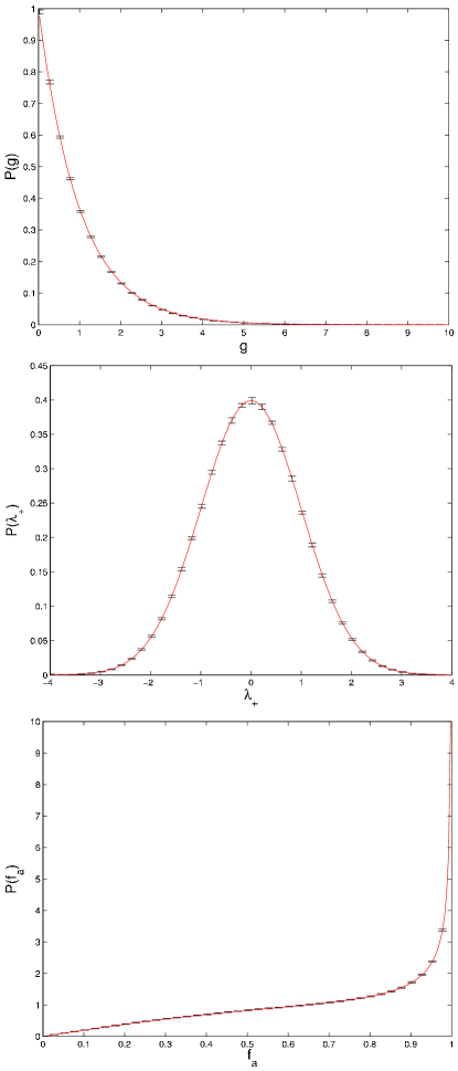
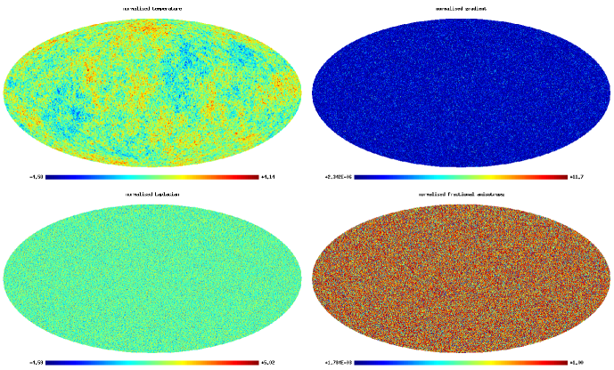
The pdfs of the three normalilzed scalars can be seen in Fig. 2. Maps of the same scalars for a random realization of a IGRF are shown in Fig. 3.
III Physical effects producing deviations from the standard IGRF
There are a number of physical effects which may produce deviations from the standard IGRF. They are normally related to secondary anisotropies produced by photon scattering, gravitational effects generated by the non-linear evolution of the matter density, variations from standard inflation in the early universe, topological defects, non-standard geometry and topology of the universe or primordial magnetic fields. Below we sumarize some relevant aspects of the most studied effects.
III.1 Secondary anisotropies
On the last scattering surface CMB anisotropies are generated via the gravitational potential (Sachs-Wolfe effect, SW ) and the physics of the baryon-photon plasma. These anisotropies are usually refered to as primary anisotropies. After matter-radiation decoupling when the temperature drops below , new anisotropies are generated during the trip made by the CMB photons to reach us. These secondary anisotropies can be originated via the gravitational redshift suffered by the photons when crossing the gravitational potentials produced by the large-scale matter distribution, or by the scattering of the microwave photons with the ionised matter after the reionization epoch (). The gravitational potential can produce two types of effect: the gravitational redshift suffered by the photons when they cross the varying potential wells formed by the matter evolution (Rees-Sciama effect, RS ; martinez-gonzalez_sanz_90 ), and the lensing effect produced by the same gravitational potentials which bends their trayectory (see e.g. Bartelmann and Schneider 2001 for a review). The CMB power spectrum produced by the Rees-Sciama effect is subdominant on all angular scales sanz_96 ; hu_dodelson_02 , and the expected 3-point correlations have an amplitude much below the cosmic variance mollerach_95 . The lensing effect produces a smoothing of the acoustic peaks in the CMB power spectrum seljak_96 ; martinez-gonzalez_97 . It also induces high-order correlations in the CMB temperature and polarization fields hu_00 .
The scattering of the CMB photons with the ionised medium produces a randomisation of the directions of the rescattered photons, implying a supression of the primary CMB anisotropies whose resulting power spectrum depends on the Thompson optical depth as . In addition, new anisotropies are generated by the scattering with the free electrons moving along the line of sight which produces a Doppler effect. This effect is strongly suppressed due to the cancellation of velocities along the line of sight. However the Doppler effect can survive cancellation if it is modulated by either density or ionization fluctuations. Its amplitude is given by:
| (24) |
In this formula is the Thompson cross-section, the electron density and the line of sight velocity of the electrons. can be further expressed as where is the mean electron density, the density fluctuation and the ionisation fraction. Two second order effects generating secondary anisotropies appear in this formula. The first one is the Doppler effect modulated by the density variation and known as Ostriker and Vishniac effect in the linear regime OV ; vishniac_87 . The second effect is the Doppler effect modulated by the ionisation fraction and is usually referred to as patchy reionization (see e.g. aghanim_96 ). Since they are of second order, both effects produce non-Gaussian perturbations in the CMB. However, their amplitude is much smaller than the thermal and kinetic Sunyaev-Zeldovich effects (SZ) SZ generated in the non-linear regime at lower redshifts and produced by the scattering of hot, ionised gas associated to collapsed structures. In addition to temperature anisotropies, due to the primary quadrupole moment reionisation also produces polarisation.
For more details about secondary anisotropies the reader is refered to e.g. hu_dodelson_02 and aghanim_puget_06 .
III.2 Non-standard models of the early universe
III.2.1 Non-standard inflationary models
In the standard, single field, slow roll inflationary model, the dominant linear effects in the evolution of density fluctuations preserve the initial Gaussian distribution produced by the quantum fluctuations of the inflaton. On the contrary, second-order effects perturb the original Gaussianity of the fluctuations, although resulting in a negligible effect in the standard model. In non-standard inflationary models, primordial non-Gaussianity should be added to the second-order effects associated to the evolution of density fluctuations after inflation finishes. In any case, it is common to characterize phenomenologically the deviations from Gaussianity by introducing the parameter in the gravitational potential komatsu_spergel_01 :
| (25) |
where is the gravitational potential at the linear order and it is distributed following a Gaussian random field. In general the non-linear couplig parameter is a function of the distance vectors and the product is really a convolution. However, an effective which accounts for those complexities can still be used. A detailed study of the values of for several non-standard inflationary models, including multi-field inflation, the curvaton scenario, inhomogeneous reheating and the Dirac-Born-Infeld (DBI) inflation inspired by string theory, can be found in bartolo_04 (see also matarrese_08 in this volume). Here it is worth noticing that sometimes the specific parameter given by eq. 25 is called the local non-linear coupling parameter , refering to the fact that is obtained from at the same position in space. In addition to which contains mainly information of the squeezed configurations (those with two large and similar wave vectors and the other small), the equilateral non-linear coupling parameter is used to caracterize equilateral configurations of the bispectrum for which the lengths of the three wave vectors are equal in Fourier space. The two non-linear coupling parameters suppose a fair representation of a large class of models. For instance, can be generated in curvaton and reheating scenarios whereas can be produced in DBI inflation within the context of String theory.
In the standard single-field slow-roll inflation the effective is dominated by second-order gravitational corrections leading to values of order unity. These low values require very sensitive measurements to be detected and are not even within reach of the Planck mission. Non-standard inflationary models generally predict larger values, some of them already constrained by WMAP. A positive detection of would rule out the standard inflationary models.
For an ideal experiment with white noise, no foreground residuals and no Galactic and point source mask, it has been shown that the optimal estimator for is based on a bispectrum test constructed from a cubic combination of appropriately filtered temperature and polarization maps komatsu_05 ; creminelli_06 ; yadav_07a . An extension to this estimator to deal with data under realistic experimental conditions has been made by yadav_07b . Several observational constraints on have been derived from different experiments. The first ones were obtained with COBE-DMR komatsu_02 ; cayon_03 . Further constraints have been derived with other experiments like VSA smith_04 , BOOMERANG troia_07 and Archeops curto_07 ; curto_08 . However, the best limits have been derived with the various releases of the WMAP data komatsu_03 ; spergel_07 ; komatsu_08 representing an improvement of at least an order of magnitud over previous ones (see below).
III.2.2 Topological defects
In standard theories of particle physics the fundamental forces of nature unify progressively when the energy scale exceeds certain thresholds. These unified theories imply that the universe went through several phase transitions during the early stages of its evolution. At energies above GeV, the electromagnetism and the weak nuclear force are merged into the electroweak force. At higher energies of the order of GeV it is believed that the electroweak force unifies with the strong nuclear force, a process usually called Grand Unified Theory (GUT). At even higher energies it is speculated that it is possible to merge gravity with the other three interactions.
Unified theories are based on symmetry. When the symmetry is broken spontaneously via the Higgs mechanism, topological defects generically appear kibble_76 (for a more pedagogical discussion about topological defects see vilenkin_shellard_00 ). Depending on the dimensionality of the symmetry which is broken, a type of topological defect is formed. When a discrete symmetry is broken domain walls form, in a two-dimensional symmetry breaking cosmic strings appear, monopoles form when the symmetry breaking is three-dimensional and textures appear when it is in four or more dimensions. In the 1980s topological defects were considered as an alternative scenario to inflationary quantum fluctuations for the process of structure formation. CMB observations showed that the former scenario could only play a subdominant role as the source of cosmic structure. Moreover, due to the catastrophic effects that the presence of domain walls and monopoles would have on our universe only the existence of cosmic strings and textures is usually considered.
A lot of effort has been made to study the cosmological consequences of cosmic strings. It is generally believed that the best strategy to detect them is by searching for their imprint on the CMB maps. The non-Gaussian character of the density field of strings produce line discontinuities in the CMB anisotropies at arcmin angular scales as a consequence of the metric deformation around the strings (the Kaiser-Sttebins effect kaiser_stebbins_84 ). However, at larger angular scales a Gaussian distribution emerge from the central limit theorem.
Cosmic textures were first studied in detail by turok_89 . They are much more diffuse than the other defects which are localized at a point (monopole), on a line (cosmic string) or a surface (domain wall). Contrary to the others, they are unstable and consist of twisted configurations of fields which collapse and unwind. Each texture creates a time-varying gravitational potential which produces red- or blue-shift to the CMB photons passing through such a region. Thus, textures generate hot and cold spots on the CMB anisotropy maps whose amplitude is set by the symmetry breaking energy scale. The shape of the spots is approximately spherically symmetric and an approximated analytical formula has been derived by turok_spergel_90 . Recently, a very cold spot detected in the WMAP temperature map has been found to be consistent with the effect produced by a texture cruz_07 . If confirmed, this result will have outstanding consequences in our understanding of the universe (see Sec. VI.6.2 for more details on this finding).
III.3 Non-standard geometry and topology
The geometry of the observable universe is believed to be well approximated on large scales by a Friedmann-Lemaitre-Robertson-Walker (FLRW) metric characterized by a homogeneous and isotropic space-time. Support for the homogeneity of the universe is provided by the largest surveys of the galaxy distribution (e.g. SDSS DR6 adelman-mccarthy_08 , 2dFGRS colless_01 ) and by the smallness of the CMB temperature fluctuations. The cosmological principle, stating that the universe is homogeneous and isotropic on large scales, follows from those observations and the assumption that we are not located at a special place in the universe (the Copernican principle).
However, recent observations of the CMB as measured by the WMAP satellite might question the cosmological principle. They are the large scale power asymmetry found between the two hemispheres of a reference frame close to that of the ecliptic one eriksen_04a ; hansen_04a , the planarity and alignment of the low multipoles oliveira-costa_04 ; land_magueijo_05a , the non-Gaussian cold spot present at scales of vielva_04 ; cruz_05 and the alignment of local structures also at similar scales wiaux_06 ; vielva_07a (see Sec. VI for more details). These results may imply the existence of priviledged directions in the CMB map and thus motivates the study of alternatives to the standard FLRW metric.
An interesting class of alternative models is that for which the metric is homogeneous but anisotropic. They are known as Bianchi models and are classified acording to their space-time properties. Their predictions for the CMB anisotropy were studied in barrow_85 . Since the signatures left by those models appear on large angular scales, they have been already constrained by the COBE-DMR experiment data martinez-gonzalez_sanz_95 ; bunn_96 ; kogut_97 . One particularly interesting case is Bianchi VIIh which experiences anisotropic expansion and global rotation. These two properties produce a characteristic pattern in the CMB in the form of a spiral pattern and spots. This model has been recently used to account for some of the large scale WMAP anomalies mentioned above jaffe_05 ; jaffe_06a ; jaffe_06b ; bridges_07a (see Sec. VI.6.1 for more details). An important problem with this model comparison approach is that the CMB anisotropies are not computed in a self-consistent way but are assumed to be the sum of two independent components: an isotropic one produced by the energy-density fluctuations which is assumed to be the same than for the FLRW model, and an anisotropic component which is the determinisitc effect produced by the anisotropic model.
A different source of anisotropic features in the CMB sky is the global topology of the universe. The local character of the General Theory of Relativity does not theoretically constrain it. If the topology of the universe is non-trivial (i.e. multiconnected, meaning that there is not a unique way to connect two points by geodesics) then CMB photons originated from the same location on the last scattering surface can be observed in different directions. This effect manifests itself in the CMB sky as anisotropic patterns, correlated (matched) circles cornish_04 or, more generically, as deviations from a IGRF (for a discussion on different topologies and tests developed to detect them see the reviews by lachieze-rey_luminet_95 and levin_02 ). An additional consequence of a multiconnected universe is the lack of fluctuations in the CMB above the wavelength corresponding to the size of the universe. This property has led to several authors to suggest that the low quadrupole and the alignment of the low multipoles measured by WMAP might be an evidence of a non-trivial topology luminet_03 ; cresswell_06 . Constraints on the topology of the universe started with the COBE-DMR data oliveira-costa_96 ; roukema_00 ; rocha_04 and followed with the WMAP data inoue_sugiyama_03 ; kunz_06 ; kunz_08 ; phillips_kogut_06 ; niarchou_jaffe_07 . All those analyses concluded that the WMAP data do not show any evidence of multiconnected universes.
III.4 Primordial magnetic fields
In recent years there has been an increasing interest in studying the consequences that the possible existence of primordial magnetic fields might have on the CMB. Magnetic fields of order of a few G have been measured in a wide range of astrophysical structures, from individual galaxies han_02 to galaxy clusters kronberg_04 . It is also widely beleived that they are present in superclusters. Although the origin of those magnetic fields is still unclear and their existence does not necessarily imply a primordial origin, studying the interplay between magnetic fields and CMB is justified by the important consequences that it may have on the CMB temperature and polarization anisotropy, and also on the distorsion of the blackbody spectrum (for reviews on this topic the reader is referred to giovannini_04 ; durrer_07 ). In particular, the presence of magnetic fields introduce non-Gaussianity in the CMB anisotropy since its amplitude depends on the square of the magnetic field intensity.
Two very different cases can be considered for the primordial magnetic field: a uniform field and a stochastic one. The former breaks the spatial isotropy of the background geometry by introducing shear through an anisotropic stress. This leads to the well known homogeneous and anisotropic Bianchi models barrow_85 . Since those models also imply an anisotropic CMB field, a uniform magnetic field generates phase correlations between different . The uniform magnetic field has been constrained with the CMB quadrupole and also with the phase correlations, implying comparable constraints on the magnetic field intensity of a few nG barrow_97 ; durrer_98 ; chen_04 .
The stochastic magnetic field is a more realistic scenario which can be generated during inflation. In this case the isotropy of the background geometry is preserved. Temperature and polarization anisotropies are generated through the vector and tensor modes associated to the magnetic field energy-momentum tensor. Allowed amplitudes of the magnetic field intensity of about several nG can produce a potentially observable B-mode polarization for nearly scale invariant spectra lewis_04 . This signal could be distinguished from the one generated by the inflationary gravitational wave background by its non-Gaussian character. In addition Faraday rotation induces B-mode polarization from the ordinary E-mode with the characteristic dependence.
Therefore, the presence of a primordial magnetic field can leave unambiguous inprints in the CMB anisotropy that would allow its identification with the sensitive data expected from the coming experiments.
IV Methods to test Gaussianity
Testing the Gaussianity of CMB data is not an easy task. In principle it consists in just proving the properties of the IGRF that we discussed in Sec. II.2: isotropy and multinormality. The CMB data represent a single realization of the underlying random field which for the standard model is nearly Gaussian and isotropic. In practice the analysis is complicated by the characteristics of the experiment which need to be known very precisely: calibration uncertainties, instrumental noise (white and 1/f) which is normally anisotropic in pixel space depending on the scanning strategy, beam response (usually close to Gaussian), data processing, … And by foreground contamination which demands certain previous cleaning operations in the data, requiring masking certain areas where the foregrounds are very intense and leaving some amount of residuals in the rest of the surveyed area. The result of cleaning depends on our a priori knowledge of the physical properties of the foregrounds and the component separation method used for their removal. These ingredients must be considered in the analysis by performing simulations accounting for them.
Unless one is interested in the compatibility of the data with a specific alternative model for which and optimal method may be found (as specific non-standard inflation, geometry or topology), there are infinite ways in which a random field can deviate from the IGRF one. Methods to test Gaussianity can be classified by the type of property that they try to prove. Typical examples are cumulants and n-point correlation functions in real space (the former should vanish and the latter either vanish for the odd order or can be expressed in terms of 2-point correlation functions for the even order), moments in spherical harmonics space (bispectrum, trispectrum, …), or moments in other spaces to which the data is transformed by linear operations which preserve Gaussianity: filters, wavelets, signal-to-noise eigenvectors, … Other approaches may test different properties of the CMB random field, like the morphology of the data using the Minkowski Functionals or the geometry of the data using scalar quantities constructed by the first and second covariant derivatives as, for example, the local curvature (see Sec. II.2). These and other methods are described in more detail in martinez-gonzalez_08 and barreiro_07 and references therein. As example of the typical statistical procedure followed in the analysis, below we focus on a few statistical methods which have been often used in the literature based on the Minkowski Functionals, bispectrum or wavelets.
As we have described in Sec. II.2, for the excursion set above a given threshold , there are three Minkowski Functionals on the sphere: total contour lenght , total area and the genus (see schmalzing_gorski_98 ). In the case of an IGRF their expected values follow simple analytical expresions as a function of (eqs. 4,5,6). However, simulations are needed to account for the experimental characteristics, basically noise, beam response and mask. As it can be shown with simulations, the 1-pdf for any Minkowski Functional at each follows a nice bell-shape distribution, implying the natural choice of a generalized as the appropriate statistical test to be used in this case to combine all the information. More specifically, considering different thresholds we can define a vector ,
| (26) |
The generalized statistic to test the Gaussianity of a data map can be then constructed as
| (27) |
where is the expected value for the Gaussian case and is the covariance matrix, , both of them usually constructed with simulations. For testing the compatibility of the data with a non-Gaussian model (e.g. a non-standard inflationary model characterized by the parameter) we simply have to use the corresponding expected value and covariance matrix for the Minkowski Functionals at different thresholds in eq. 27. If the deviations from Gaussianity are small (as in the case of the models with ) the covariance matrix can be well aproximated by the one of the Gaussian case. More information is added to the analysis by considering different resolutions of a given data map. Including this extra information simply increases the vectors and covariance matrix present in the expression to a dimension . Examples of applications of this method to different data sets can be found in komatsu_03 for the 1-year WMAP data, troia_07 for the BOOMERanG 3-year data and curto_08 for the Archeops data. Recently, perturvative formulae of the Minkowski Functionals as a function of have been derived for the models hikage_06 . The results of applying them to the 3-year WMAP data show constraints on very similar to the ones obtained with the optimal bispectrum hikage_08 .
Generically, non-standard models of inflation produce small deviations of Gaussianity which are more prominent in the 3-point correlation function or equivalently, its harmonic transform the bispectrum . The trispectrum, the harmonic transform of the 4-point correlation function, can also play an important role in discriminating inflation models since some models do not produce any bispectra but produce significant trispectra, or produce similar amplitudes of the bispectra but very different trispectra (e.g. DBI inflation, huang_shiu_06 , or New Ekpyrotic Cosmology, buchbinder_07 ). Here we briefly describe the bispectrum, for more details on it and the trispectrum see komatsu_01 . The average bispectrum, , is the rotationally invariant third order moment of spherical harmonic coefficients and is given by the following expresion (see hu_01 and bartolo_04 for more details on this and higher order moments):
| (28) |
where is the Wigner-3j symbol. The bispectrum must satisfy the selection rules. Rotational invariance of the 3-point correlation function implies that the bispectrum can be written as
| (29) |
where is the Gaunt factor and is a real symmetric function of , and called the reduced bispectrum. By substituting eq. 29 in eq. 28 it is straight forward to obtain the following relation between the averaged bispectrum and the reduced bispectrum
| (30) |
Therefore under rotational invariance the reduced bispectrum contains all physical information of the bispectrum. In particular is fully identified by the inflationary models characterized by the non-linear coupling parameter . Thus these models can be optimally tested by using the averaged bispectrum. The computation of the full averaged bispectrum scales as , where is the number of pixels, and is already not feasible for the WMAP data. komatsu_05 solved this problem by constructing a cubic statistic, the KSW estimator, that combines the triangle configurations of the bispectrum optimally for determining , with its computation scaling as . The extension of this estimator to , and also including polarization, has been made in creminelli_06 and yadav_07a . The strongest constraints on the non-linear coupling parameter up to date have been obtained by applying the KSW estimator to the WMAP data (see next section).
Wavelets are compensated filters which allow one to extract
information which is localized in both real and harmonics
space. In particular wavelets may provide information on the position
and scale of different features in astrophysical images. They
can be more sensitive than classical methods (for a review on wavelets
see jones_08 and for applications to the CMB see
vielva_07b ). One example which has been used many times in
cosmological applications is the Mexican hat wavelet defined as the
Laplacian of a Gaussian function. For CMB analyses the extension of an
Euclidean wavelet to the sphere can be made with an inverse stereographic
projection antoine_vandergheynst_98 . By this procedure the
spherical Mexican hat wavelet can be constructed preserving dilation and
compensation martinez-gonzalez_02 , and was first applied to
CMB analyses by cayon_01 using COBE-DMR data. Also it can be made
directional, i.e. sensitive not only to the scale but also to the
orientation of a feature, by simply considering different widths along
the two axes of the original 2-dimensional Gaussian.
A very useful property to study directional properties of structures in
an image is the so called steerability. In general, a directional or
non-axisymmetric filter is said to be steerable
if any rotation about itself can be expressed as a finite linear
combination of non-rotated basis filters. This concept has been recently
extended to the sphere by wiaux_05 . An important consequence of
the steerability property is that it makes the wavelet analysis very
efficient computationally (see Sec. VI.4). An
interesting spherical steerable
wavelet is the second Gaussian derivative one which may be rotated in
terms of three basis wavelets: the second derivative in direction x,
the second derivative in direction y, and the cross-derivative. This
wavelet provides information on the three local morphological measures
of orientation, signed intensity (amplitude at the orientation which
maximizes the absolute value of the coefficient) and elongation. It
has been recently applied to the CMB analysis to test global isotropy
and Gaussianity wiaux_06 ; wiaux_08 ; vielva_07a
(see Sec. VI.4).
V Constraints from observations
Previously to any Gaussianity study, one major problem in the analysis of the observational data is the separation of the different Galactic and extragalactic components from the CMB itself. A key property to distinguish them is the frequency dependence of the specific emission in the microwave range. Thus, the intensity of the Galactic synchrotron and free-free emissions decreases with frequency as a power-law with approximated spectral indexes and , respectively. On the contrary, the intensity of the Galactic thermal dust increases with frequency following approximately a grey-body spectrum with emissivity and temperature K. Extragalactic sources emitting in the microwave band are typically radio galaxies and IR galaxies, with their emission dominating at frequencies GHz for the former (synchrotron-like) and at higher ones (dust-like) for the latter. An additional extragalactic emission comes from galaxy clusters through the SZ effect, as was discussed in Sec. III.1. The spatial distribution of the different foregrounds is also very different from the CMB one, differing very much from that of an IGRF. Thus, the Galactic foreground emissions dominate at large angular scales with the power spectrum of fluctuations decaying approximately as . On the contrary the extragalactic foregrounds dominate at the smallest angular scales and appear as point sources for typical CMB experiments. (For more details on the properties of foregrounds see contributions by davies_08 and partridge_08 to this volume). All these properties have to be exploited in order to best disentangle the foreground emissions from the CMB one. Indeed, the numerous component separation methods already developed take advantage of our knowledge of those foreground properties to obtain a clean CMB map (see delabrouille_cardoso_08 and barreiro_08 for further reading on this topic).
The Gaussianity of the CMB signal has been studied with data measured by many different experiments. The first systematic analysis was carried out with the all-sky COBE-DMR satellite smoot_92 ; bennett_94 . Other analyses were based on data covering a fraction of the sky and obtained from experiments onboard stratospheric balloons, like QMAP, MAXIMA, BOOMERanG or Archeops, and from ground-based ones like Saskatoon, QMASK or VSA. The result of most of those Gaussianity studies was a systematic compatibility with the standard IGRF. Deviations were also claimed in a few cases which were later proved to be due to either systematics or an incomplete analysis. Upper limits on the parameter were derived of approximately a few thousands komatsu_02 ; cayon_03 . For a more detailed discussion on those analyses see martinez-gonzalez_08 . A significant improvement has been recently achieved with measurements by BOOMERanG and Archeops, lowering the upper limit to at the c.l. troia_07 ; curto_08 . It is worth mentioning a deviation from the IGRF found in one of the VSA fields, the Corona Borealis supercluster genova-santos_05 ; rubino-martin_06 . The deviation consists in a strong and resolved negative spot, of K and angular size of arcmin, which is not associated with any of the clusters of that supercluster. A SZ effect produced by a diffuse, extended warm/hot gas distribution has been suggested as a possible explanation genova-santos_08 . This hypothesis, if confirmed, would be of relevance for providing the location of the missing baryons in the local universe.
The precision with which the Gaussianity of the CMB can be tested has been strongly improved with the quality data measured with the WMAP satellite bennett_03a ; hinshaw_07 ; hinshaw_08 . The WMAP team has provided “cleaned” CMB maps at the Q, V and W frequency bands for the 5 year data collected by the experiment, and masks covering a region around the Galactic plane and a catalogue of radio sources where the foreground emission cannot be removed at the required sensitivity. By a noise-weighting combination of the cleaned maps at the cosmological frequencies and applying a conservative mask the WMAP team has performed a Gaussianity study of the data based on the Minkowski Functionals and the optimal bispectrum. For both quantities the 1, 3 and 5-year WMAP data releases have been found to be compatible with the IGRF komatsu_03 ; spergel_07 ; komatsu_08 . Stringent limits have been also derived on the local and equilateral parameter using an optimal bispectrum-like quantity: and at the c.l.
VI WMAP anomalies
The WMAP team found the WMAP data consistent with the IGRF using the Minkowski functionals and the bispectrum. Subsequently, many works have tested the Gaussianity of the WMAP data in many different ways. Some of them have found agreement with Gaussianity whereas others found significant deviations of the IGRF. Examples of the former are analyses based on 3-point correlation analysis gaztanaga_wagg_03 ; chen_szapudi_05 , integrated bispectrum cabella_06 , real space statistics bartosz_08 or isotropy analyses based on the Bipolar power spectrum hajian_05 ; hajian_souradeep_06 . Examples of the latter are analyses based on phase correlations chiang_03 , the genus park_04 , isotropic wavelets vielva_04 ; mukherjee_wang_04 ; cruz_05 , 1-pdf monteserin_07 , isotropy analyses based on local n-point correlations eriksen_04a , local curvature hansen_04b , multipole vectors copi_04 ; copi_07 or directional wavelets mcewen_05 ; wiaux_06 ; vielva_07a ; wiaux_08 . However, some of the analyses have been performed on the whole sky internal linear combination (ILC) map bennett_03b or similar maps (e.g. TOH ) which is well known to suffer from Galactic contamination and, as stated by the WMAP team itself, should not be used for cosmological analyses. From here on, we will concentrate on the most relevant works based on WMAP maps where a certain region around the Galactic plane has been masked as well as several hundred of extragalactic sources. The deviations or “anomalies” reported have been detected using other statistical quantities different from the ones originally used by the WMAP team. They are the North-South asymmetry eriksen_04a ; hansen_04a , alignment of the low multipoles oliveira-costa_04 ; land_magueijo_05a , the cold spot vielva_04 ; cruz_05 ; cruz_07 , non-Gaussian features detected with directional wavelets mcewen_05 ; mcewen_08 , alignment of CMB structures wiaux_06 ; vielva_07a , low variance monteserin_07 . Below we describe these anomalies and discuss several relevant aspects like significance, origin, etc.
VI.1 North-south asymmetry
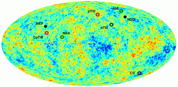
North-South asymmetries in ecliptic coordinates have been observed in the WMAP CMB maps using several local quantities: power spectrum and 2 and 3-point correlation functions eriksen_04a ; eriksen_05 , Minkowski functionals eriksen_04b , local power spectrum hansen_04a ; donoghue_donoghue_05 , local bispectra land_magueijo_05b and local curvature hansen_04b . Varying the coordinate system, a maximum asymmetry for the two hemispheres is obtained for a system whose north pole is lying at . This direction is close to the north ecliptic pole (see Fig. 4). The result of all those works basically indicates a significant lack of power in the north ecliptic hemisphere compared to the south one. The asymmetry has been also confirmed by bernui_06 ; bernui_07 using a pair angular separation histogram method.
The asymmetry remains stable with respect to variations in the Galaxy cut and to the frequency band. Also a similar asymmetry is found in the COBE-DMR map with the axis of maximum asymmetry close to the one found in the WMAP data. Analyses of the possible foreground contamination and known systematics do not seem to be the cause of such asymmetry eriksen_04a .
More recently, the asymmetry has been found again in the 3-year WMAP CMB map eriksen_07 .
VI.2 Alignment of the low multipoles
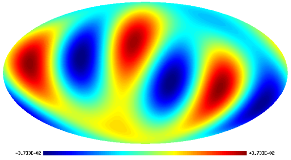
The lowest mulpoles, especially , of the WMAP data have been found to be anomalously planar and aligned copi_04 ; copi_07 ; oliveira-costa_04 ; katz_weeks_04 ; schwartz_04 ; bielewicz_05 . In Fig. 5 the quadrupole and octopole of the ILC map are shown. Both multipoles present maxima and minima following a planar shape, whose perpendicular axis points towards similar direction called axis of evil. The axes of the two multipoles are separated by . The probability that the two directions are separated by that angle or less by chance is . Further alignments have also been claimed for higher multipoles land_magueijo_05a and freeman_06 . The northern end of the alignment points towards , a direction close to the CMB dipole one whose northern end is at (see Fig. 4).
A problem which appears when trying to estimate the low multipole components is that they are very much affected by the mask. Varying the mask produces significant changes in their amplitude estimates, especially for the quadrupole, implying consequently uncertainties in the determination of their axes. Detailed analyses of this effect tend to weaken the significance of the detection oliveira-costa_06 ; land_magueijo_07 .
VI.3 The cold spot
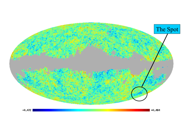
A large and prominent cold spot has been observed in the WMAP data which is hard to explain within the standard inflationary scenario. It was detected with the SMHW as defined in martinez-gonzalez_02 . The first evidence came from the kurtosis of the wavelet coefficients of the first-year data which showed an excess with respect to the Gaussian hypothesis at a wavelet scale of (corresponding to a structure size of ) vielva_04 . A very cold spot at Galactic coordinates was identified as the possible source of the excess (see Fig. 6). An analysis of the area of the spots at different thresholds in the SMHW coefficient map at around proved that indeed the cold spot had a very large area and was the source of the excess of the kurtosis cruz_05 .
The cold spot has been also shown to deviate from Gaussianity using the Max and Higher Criticism estimators cruz_05 ; cayon_05 . A study of the morphology of the spot with the elliptical MHW on the sphere has found an almost circular shape cruz_06 . In the same paper the possible foreground contribution was considered in detail, concluding that contributions from the SZ effect and the Galaxy had to be negligible.
The cold spot has been also identified as the most prominent spot in the CMB sky using steerable wavelets vielva_07a . In that work two other spots are identified as deviations from the IGRF three-year WMAP best fitting model. However, the deviation from Gaussianity seen in the kurtosis of the coefficients of that wavelet wiaux_08 cannot be assigned exclusively to those three spots.
mcewen_05 ; mcewen_08 have also detected a number of non-Gaussian features, including the cold spot, using the directional wavelets elliptical Mexican hat and Morlet.
All the previous results have been confirmed with the 3-year WMAP CMB map cruz_07 and are expected to be almost unaltered for the 5-year data.
VI.4 Alignment and signed-intensity of local structures
Some of the previous anomalies imply preferred directions in the sky that, under the assumption of Gaussianity, represent deviations from statistical isotropy. Here we describe a different violation of statistical isotropy based on the alignment of CMB structures. The structures are identified by convolving the CMB map with the steerable wavelet formed by the second Gaussian derivative wiaux_05 . For each scale and position in the sky the wavelet identifies the orientation which maximizes the absolute value of the wavelet coefficients. Thus this orientation corresponds to the characteristic orientation of the local feature of the signal. The wavelet coefficient in that specific orientation defines the so-called signed-intensity vielva_07a . It should be remarked that these two quantities, local orientation and signed-intensity, are computationally feasible because of the steerability property (see Sec. IV).
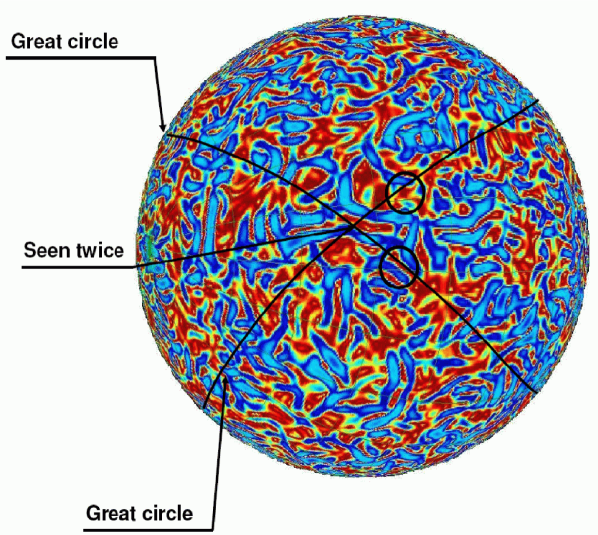
Once the local orientation is determined for every position in the sky at a given scale, we can construct the following isotropy test. First, the great circle passing by that position and tangent to the local orientation is identified. Every other pixel which is now crossed by that great circle is considered to be seen by the local orientation of the first position (this procedure is illustrated in Fig. 7), with a weight naturally given by the absolute value of the signed-intensity of the first position. Second, we can assign to each pixel in the sky the total weight given by the sum of the weights of all the pixels which see that pixel. This new total weight signal is even under parity and thus its analysis can be restricted to one hemisphere of reference. The highest total weights represent the positions towards which the CMB features are predominantly directed while the lowest ones represent the positions predominantly avoided by the CMB features. Of course, for an all-sky IGRF all the pixels should have the same total weight on average.
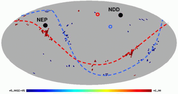
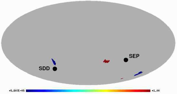
This isotropy test based on the alignment of local orientations has been applied to the first wiaux_06 and three-year vielva_07a WMAP data. In both cases a significant violation of isotropy was found at a scale around . The highest total weights (above ) define an axis located very close to the ecliptic one. The highest and the lowest total weights define two planes whose normal axes are close to the CMB dipole one (Fig 8).
Besides the alignment of the local orientations, an analysis of the signed-intensities show three spots at angular scales also around containing a total of 39 -pixels whose values have a (signal+noise) probability in the tails (see Fig. 9). This pattern is similar to the one found with the axisymmetric Mexican hat wavelet vielva_04 . The three spots are located in the southern galactic hemisphere confirming the north-south asymmetry. Two of the them are cold, one being identified with the cold spot already detected in vielva_04 .
The two anomalies which appear at similar scales, with global significance levels around per cent, are however quite independent.
VI.5 Low variance
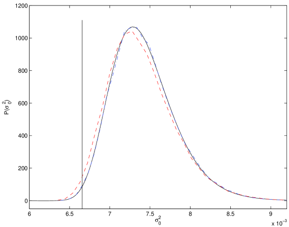
Very recently monteserin_07 the 1-pdf of the WMAP three-year data has been analysed finding an anomalous low value of the variance as compared to the one expected from the WMAP best-fit cosmological model. The result is even more prominent if only the north ecliptic hemisphere is considered (see Fig. 10), in agreement with the lack of power found in that hemisphere by previous works (see e.g. eriksen_04a ). The variance of the CMB signal is obtained by fitting the normalized temperature distribution to a Gaussian of zero mean and unit variance. The significance of the result is around (see Fig. 11).
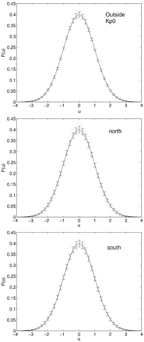
In order to find a possible origin for this anomaly the behaviour of single radiometer and single year data as well as the effect of residual foregrounds and 1/f noise have been studied. None of these possibilities can explain the low value of the variance.
Since the largest contribution to the variance comes from the lower multipoles, it is interesting to see if the low quadrupole measured by COBE and WMAP is the cause of the anomalously low variance. Performing the same analysis after subtracting the best-fit quadrupole outside the Kp0 mask the significant of the result is slightly reduced although the variance is still anomalously low.
Beyond the inconsistency found between the best-fit model and the measured variance, one could ask if the latter is consistent with the actual measured power spectrum of the WMAP data. The analysis performed by the same authors show that a strong discrepancy is indeed found. This last result suggests a possible deviation of the CMB data form the IGRF.
VI.6 Cosmological consequences
Given that neither foreground contamination nor known systematics seem to be causing most of the previous anomalies, there has been a number of attempts to explain the cause of the WMAP anomalies by an intrinsic origin. Among them we mention the Rees-Sciama effect produced by large voids tomita_05 ; inoue_silk_07 ; rudnick_07 , inhomogeneous adler_06 ; land_magueijo_06 or anisotropic universes jaffe_05 and cosmic defects cruz_07 . Although no further evidence has been found for those explanations most of them still remain as plausible. Below we discuss in more detail two interesting possibilities: the Bianchi model and the cosmic texture.
VI.6.1 Bianchi model
A first interesting attempt to explain the best studied WMAP anomalies was performed by jaffe_05 ; jaffe_06a who suggested that such features might be produced by an anisotropic universe, the Bianchi VIIh model. This type of model has a global anisotropic expansion and vorticity that produces geodesic focusing and a spiral pattern in the CMB anisotropy at large angular scales. By fitting the free parameters of that model to the WMAP map the large scale CMB anisotropies produced by its non-standard geometry are determined. After subtracting that pattern from the WMAP data, the best studied WMAP anomalies, namely the low-multipole alignments, the north-south asymmetry and the cold spot, were significantly reduced.
This result seemed to suggest that the universe was not well represented by the homogeneous and isotropic FLRW model and that a perturbation in the form of a Bianchi VIIh was a better representation. However, a more detailed examination of the best-fitted parameters of the Bianchi model when a dark energy was included showed values of the dark energy and matter energy density far from the ones measured by many current cosmological tests jaffe_06b ; bridges_07a . Considering other Bianchi models with vorticity and shear, like the Bianchi IX with a closed geometry, do not help since they do not exhibit geodesic focusing or the spiral pattern.
Very recently, bridges_07b computed the Bayesian evidence of the Bianchi template when the cold spot was not included in the analysis (see below for an alternative interpretation of the cold spot). The result was that the evidence was now significantly reduced, reinforcing the idea that the cold spot was likely to be driving any Bianchi VIIh detection.
VI.6.2 The cold spot texture
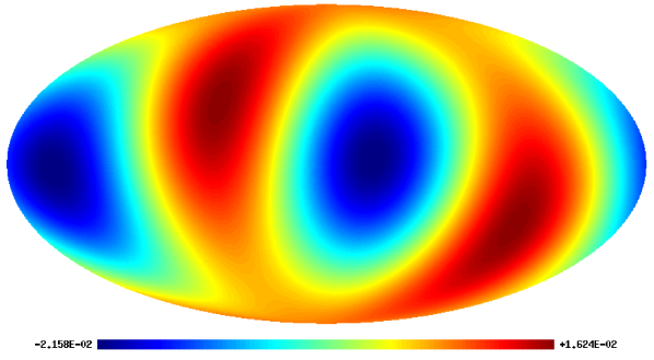
Recently, cruz_07 performed a Bayesian evidence analysis to test the hypothesis that the cold spot is produced by a cosmic texture. This is a type of toplogical defect that, as explained in Sec. III.2.2, in the standard theories of unification of the fundamental forces of nature, are expected to appear in the early universe. The motivation for considering a texture as the origin of the cold spot is its typical spherical anisotropy pattern left in the CMB and the relatively small number of spots expected at scales of several degrees (see Fig. 12).
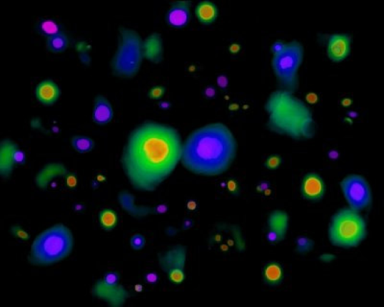
The hypothesis test considered consisted in the comparison of the following two hypotheses: the null hypothesis for which the cold spot is just a rare fluctuation of the IGRF predicted by the standard inflationary model, and the alternative hypothesis, for which on top of the inflationary Gaussian CMB fluctuations there are non-Guassian ones as produced by the texture model. The test is applied to a circular area of diameter centered on the cold spot position. The posterior probability ratio of the two hypotheses is:
| (31) |
where is the data vector, and the evidence which is the average likelihood with respect to the priors in the parameters of the hypothesis ,
| (32) |
and is the a priori probability of hypothesis . The a priori probability ratio is usually set to unit for lack of information, but since in our case the analysis is centered in the cold spot (an a posteriori selected pixel) it should be given by the sky fraction covered by textures. Given that a scale-invariant distribution of spots is expected and considering only textures above (photon difusion would smear out textures smaller than that) . The likelihood funtion is simply where and is the CMB+noise covariance matrix. The anisotropy pattern produced by a texture can be approximated by an analytical spherical profile vilenkin_shellard_00 with only two free parameters: the amplitude which is related to the fundamental symmetry-breaking energy scale, and the angular scale which is related to the redshift when the texture unwinds.
The result of the analysis is a probability ratio for the three-year WMAP data, favouring the texture hypothesis (see Fig 13 for the resulting best-fit texture template). This result is slightly increased () for the five-year data due to the reduction in the noise amplitude. The texture interpretation helps to alleviate the excess found in the kurtosis, being at the same time compatible with the observed abundance, shape, size and amplitude of the spot. In particular, the symmetry-breaking scale inferred from this analysis, GeV, is compatible with the upper limit obtained from the CMB power spectrum analysis bevis_04 .
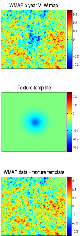
More recently, cruz_08 have extended the Bayesian evidence analysis to models based on the Rees-Sciama effect produced by voids or on the SZ effect. The result is that, contrary to the texture model, no positive evidence is found for those models.
VII Concluding remarks and future perspectives
The main conclusion derived from the large amount of analyses, involving a variety of methods, performed to test the Gaussianity of the CMB anisotropies, specially those measured by WMAP, is that the standard IGRF prediction is a good representation of their properties as a first approach. Furthermore, a number of significant deviations from the ideal IGRF has also been reported whose origin and interpretation is still under debate. Some of them might have to do with foreground residuals or unknown systematics while others could be a hint of new physics with profound implications for our understanding of the universe. Probably, to answer those questions we will have to wait for new data coming from the advanced experiments being built and expected to be operative in the next years.
Future experiments will shed light on the open questions remaining from the up-to-date analyses of the CMB data, specially on the WMAP anomalies discussed in Sec. VI. In particular, the Planck mission is expected to provide all-sky, high quality, multifrequency maps in the frequency range GHz. The wider frequency range and the higher sensitivity and resolution will allow an improvement in the quality of the resulting CMB map. As a consequence, an improvement in the control of the foreground emission is expected as well as a reduction in the sky area required to be masked. In addition to the temperature, improvements are also expected in the polarization maps which will be provided by Planck, meaning an important complement for probing the nature of the anomalies as well as for testing the different physical interpretations proposed for them. Missions for measuring polarization at the highest sensitivity allowed by present technology, and with the main aim of probing the existence of the gravitational wave background, have been recently proposed to both agencies, ESA and NASA. As for the temperature, the linear polarization expected to be produced as a consequence of the standard inflationary period of the universe also posseses properties very close to those of the IGRF studied in Sec. II. Therefore, extensions of the methods already discussed in Sec IV for temperature are also expected to be applied to test the Gausianity of the future polarization maps.
Acknowledgements
I thank R.B. Barreiro and P. Vielva for useful comments on the
manuscript and M. Cruz, A. Curto and C. Monteserín for helping me
with some figures. I
acknowledge financial support from the Spanish MEC project
ESP2007-68058-C03-02. I also acknowledge the use of LAMBDA, support
for which is provided by the NASA Office of Space Science. The work
has also used the software package HEALPix
(http://www.eso.org/science/healpix) developed by K.M. Gorski,
E.F. Hivon, B.D. Wandelt, J. Banday, F.K. Hansen and M. Barthelmann
gorski_05 .
References
- (1) Adler, R. J., 1981, The geometry of random fields, John Wiley & Sons, Chichester
- (2) Adler R.J., Bjorken J.D. & Overduin J.M., 2006, gr-qc/0602102
- (3) Ademan-McCarthy J.K. et al., 2008, ApJS, 175, 297
- (4) Aghanim N., Desert F.X., Puget J.L. & Gispert R., 1996, A&A, 311, 1.
- (5) Aghanim N. & Puget J.L., 2006, in CMB and Physics of the early Universe, ed. G. de Zotti et al., Proceeding of Science
- (6) Antoine J.-P. & Vandergheynst P., 1998, J. Math. Phys. 39, 3987
- (7) Barreiro R.B., Sanz J.L., Martínez-González E., Cayón L. & Silk J., 1997, ApJ, 478, 1
- (8) Barreiro R.B., 2007, in Highlights of Spanish Astrophysics IV. Proceedings of the VII Scientific Meeting of the Spanish Astronomical Society (SEA), Barcelona, September 12-15, 2006. Ed. F. Figuras et al., Springer
- (9) Barreiro R.B., 2008, in Data Analysis in Cosmology, eds. V.J. Martínez et al., Springer
- (10) Barrow J.D., Juszkiewicz R. & Sonoda D.H., 1985, MNRAS, 213, 917
- (11) Barrow J.D., Ferreira P.G. & Silk J., 1997, Phys. Rev. Lett., 78, 3610
- (12) Bartelmann M. & Schneider P., 2001, Phys. Rep. 340, 291
- (13) Bartolo N., Komatsu E., Matarrese S. & Riotto A., 2004, Phys. Rep., 402, 103
- (14) Bartosz L., 2008, A&A, submitted, astro-ph/08031409
- (15) Basser P.J. & Pierpaoli C., 1996, J. Magn. Reson. Med. B, 111, 209-219
- (16) Bennett C.L. et al., 1994, ApJ, 436, 443
- (17) Bennett C.L. et al., 2003, ApJS, 148, 1
- (18) Bennett C.L. et al., 2003, ApJS, 148, 97
- (19) Bernui A., Villela T., Wuensche C.A., Leonardi R. & Ferreira I., A&A, 454, 409
- (20) Bernui A., Mota B., Reboucas M.J. & Tavakol R., A&A, 464, 479
- (21) Bevis N., Hindmarsh M. & Kunz M., 2004, Phys. Rev. D, 70, 043508
- (22) Bielewicz P., Eriksen H.K., Banday A.J., Gòrski K.M. & Lilje P.B., 2005, ApJ, 635, 750
- (23) Bond J.R. & Efstathiou G., 1987, MNRAS, 226, 655
- (24) Bridges M., McEwen J.D., Lasenby A.N. & Hobson M.P., 2007, MNRAS, 377, 1473
- (25) Bridges M., McEwen J.D., Cruz M., Hobson M.P., Lasenby A.N., Vielva P. & Martínez-González, 2007, MNRAS, submitted, astro-ph/07121789
- (26) Buchbinder E., Khoury J. & Ovrut B.A., 2007, hep-th/07105172
- (27) Bunn, E.F., Ferreira, P. & Silk, J. 1996, Phys. Rev. Lett., 77, 2883
- (28) Cabella P. et al., 2006, MNRAS, 369, 819
- (29) Cayón L., Martínez-González E. & Sanz J.L., 1991, MNRAS, 253, 599
- (30) Cayón L. et al., 2001, MNRAS, 326, 1243
- (31) Cayón L., Martínez-González E., Argüeso F., Banday A.J., Gorski K.M., 2003, MNRAS, 339, 1189
- (32) Cayón L., Jin J. & Treaster A., 2005, MNRAS, 362, 826
- (33) Chen G. et al., 2004, ApJ, 611, 655
- (34) Chen G. & Szapudi I., 2005, ApJ, 635, 743
- (35) Chiang L.-Y., Naselsky P.D., Verkhodanov O.V. & Way M.J., 2003, ApJL, 590, 65
- (36) Colless M.M. et al., 2001, MNRAS, 328, 1039
- (37) Copi C.J., Huterer D. & Starkman G.D., 2004, Phys. Rev. D, 70, 043515, astro-ph/0310511
- (38) Copi C.J., Huterer D., Schwarz D. & Starkman G.D., 2007, Phys. Rev. D, 75, 023507
- (39) Cornish N.J., Spergel D.N., Starkman, G.D. & Komatsu E., 2004, Phys. Rev. Lett., 92, 201302
- (40) Creminelli P., Nicolis A., Senatore L., Tegmark M. & Zaldarriaga M., 2006, JCAP, 0605, 004
- (41) Cresswell J.G., Liddle A.R., Mukherjee P. & Riazuelo A., 2006, Phys. Rev. D, 73, 041302, astro-ph/0512017
- (42) Cruz M., Martínez-González E., Vielva P. & Cayón L., 2005, MNRAS, 356, 29
- (43) Cruz M., Tucci M., Martínez-González E. & Vielva P., 2006, MNRAS, 369, 57
- (44) Cruz M., Turok N., Vielva P., Martínez-González E. & Hobson M., 2007, Science, 318, 1612
- (45) Cruz M., Martínez-González E., Vielva P., Diego J.M., Hobson M.P. & Turok N., 2008, MNRAS, submitted, astro-ph/08042904
- (46) Curto A. et al., 2007, A&A, 474, 23
- (47) Curto A. et al., 2008, A&A, submitted, astro-ph/08040136
- (48) de Oliveira-Costa A., Smoot G.F. & Starobinsky A.A., 1996, ApJ, 468, 457
- (49) de Oliveira-Costa A., Tegmark M., Zaldarriaga M. & Hamilton A., 2004, Phys. Rev. D, 69, 063516
- (50) de Oliveira-Costa A. & Tegmark M., 2006, Phys. Rev. D, 74, 023005
- (51) De Troia G. et al., 2007, ApJL, 670, 73
- (52) Delabrouille J. & Cardoso J.F., 2008, in Data Analysis in Cosmology, eds. V.J. Martínez et al., Springer
- (53) Davies R., in this volume
- (54) Donoghue E.P. & Donoghue J.F., 2005, Phys. Rev. D, 71, 043002
- (55) Doré O., Colombi S. & Bouchet F.R., 2003, MNRAS, 344, 905
- (56) Delabrouille J. & Cardoso J.F., 2008, in Data Analysis in Cosmology, eds. V.J. Martínez et al., Springer
- (57) Durrer R., Kahniashvili T. & Yates A., 1998, Phys. Rev. D, 58, 123004
- (58) Durrer R., 2007, New Astronomy Reviews, 51, 257
- (59) Eriksen H.K., Hansen F.K., Banday A.J., Gorski K.M. & Lilje P.B., 2004, ApJ, 605, 14
- (60) Eriksen H.K., Novikov D.I., Lilje P.B., Banday A.J., Gorski K.M., 2004, ApJ, 612, 64
- (61) Eriksen H.K., Banday A.J., Gorski K.M. & Lilje P.B., 2005, ApJ, 622, 58
- (62) Eriksen H.K., Banday A.J., Gorski K.M., Hansen F.K. & Lilje P.B., 2007, ApJL, 660, L81
- (63) Freeman, P.E., Genovese, C.R., Miller, C:J., Nichol, R.C. & Wasserman, L., 2006, ApJ, 638, 1
- (64) Gaztañaga E. & Wagg J., 2003, Phys. Rev. D, 68, 021302
- (65) Génova-Santos R. et al., 2005, MNRAS, 363, 79
- (66) Génova-Santos R. et al., 2008, MNRAS, submitted, astro-ph/08040199
- (67) Giovannini M, 2004, Int. J. Mod. Phys. D, 13, 391
- (68) Górski K.M., Hivon E.F., Wandelt B.D., Banday J., Hansen F.K. & Barthelmann M., 2005, ApJ, 622, 759
- (69) Hajian A., Souradeep T. & Cornish N., 2005, ApJ, 618, 63
- (70) Hajian A. & Souradeep T., 2006, Phys. Rev. D, 74, 123521
- (71) Han J. & Wielebinski R., 2002, ChJA&A, 2, 293
- (72) Hansen F.K., Banday A.J. & Gorski K.M., 2004, MNRAS, 354, 641
- (73) Hansen F.K., Cabella P., Marinucci D. & Vittorio N., 2004, ApJ, 607, L67
- (74) Hikage C., Komatsu E. & Matsubara T., 2006, ApJ, 653, 11
- (75) Hikage C., Matsubara T., Coles P., Liguori M., Hansen F.K. & Matarrese S., 2008, MNRAS, submitted, astro-ph/08023677
- (76) Hinshaw G. et al., 2007, ApJS, 170, 288
- (77) Hinshaw G., et al., 2008, ApJS, submitted, astro-ph/08030732
- (78) Huang M.-X. & Shiu G., 2006, Phys. Rev. D, 74, 121301
- (79) Hu W., 2000, Phys. Rev. D, 62, 043007
- (80) Hu W., 2001, Phys. Rev. D, 64, 083005
- (81) Hu W. and Dodelson S., 2002, ARAA, 40, 171
- (82) Inoue K.T. & Silk J., 2007, ApJ, 664, 650
- (83) Inoue K.T. & Sugiyama N., 2003, Phys. Rev. D, 67, 043003
- (84) Inoue K.T. & Silk J., 2007, ApJ, 664, 650
- (85) Jaffe T.R., Banday A.J., Eriksen H.K., Gorski K.M. & Hansen F.K., 2005, ApJL, 629, L1
- (86) Jaffe T.R., Banday A.J., Eriksen H.K., Gorski K.M. & Hansen F.K., 2006, A&A, 460, 393
- (87) Jaffe T.R., Hervik S., Banday A.J., Gorski K.M., 2006, ApJ, 644, 701
- (88) Jones B.J.T., 2008, in Data Analysis in Cosmology, eds. V.J. Martínez et al., Springer
- (89) Kaiser N. & Stebbins A., 1984, Nature, 310, 391
- (90) Katz G. & Weeks J., 2004, Phys. Rev. D, 70,063527
- (91) Khoury J., Ovrut B.A., Steinhardt P.J. & Turok N., Phys. Rev. D, 2001, 64, 123522
- (92) Kibble T.W.B., 1976, J. Phys. A, 9, 1387
- (93) Kogut A., Hinshaw G. & Banday A.J., 1997, Phys. Rev. D, 55, 1901
- (94) Komatsu E., 2001, Ph.D. thesis, astro-ph/0206039
- (95) Komatsu E. & Spergel D.N., 2001, Phys. Rev. D, 63, 063002
- (96) Komatsu E., Wandelt B.D., Spergel D.N., Banday A.J. & Gorski K.M., 2002, ApJ., 566, 19
- (97) Komatsu E. et al., 2003, ApJS, 148, 119
- (98) Komatsu E., Spergel D.N. & Wandelt B.D., 2005, ApJ, 634, 14
- (99) Komatsu E. et al., 2008, ApJS, submitted, astro-ph/08030547
- (100) Kronberg P.P., 2004, JKAS, 37, 501
- (101) Kunz M., Aghanim N., Cayón L., Forni O., Riazuelo A. & Uzan J.P., 2006, Phys. Rev. D, 73, 023511
- (102) Kunz M., Aghanim N., Riazuelo A. & Forni O., 2008, Phys. Rev. D, 77, 023525
- (103) Lachièze-Rey, M. & Luminet, J.-P. 1995, Phys. Rep., 254, 135
- (104) Land K. & Magueijo J., 2005, Phys. Rev. Lett., 95, 071301
- (105) Land K. & Magueijo J., 2005, MNRAS, 357, 994
- (106) Land K. & Magueijo J., 2006, MNRAS, 367, 1714
- (107) Land K. & Magueijo J., 2007, MNRAS, 378, 153
- (108) Levin J., 2002, Phys. Rep., 365, 251-333
- (109) Lewis A., 2004, Phys. Rev. D, 70, 043011
- (110) Longuet-Higgins, M. S., 1957, Phil. Trans. Roy. Soc. London, A, 249, 321
- (111) Luminet J.-P., Weeks J.R., Riazuelo A., Lehoucq R. & Uzan J.-P., 2003, Nature, 425, 593
- (112) McEwen J.D., Hobson M.P., Lasenby A.N. & Mortlock D.J., 2005, MNRAS, 359, 1583
- (113) McEwen J.D., Hobson M.P., Lasenby A.N. & Mortlock D.J., 2005, MNRAS, submitted, astro-ph/08032157
- (114) Martínez-González E., Sanz J.L. & Silk J., 1990, ApJL, 335, L5
- (115) Martínez-González E. & Sanz J.L., 1990, MNRAS, 247, 473
- (116) Martínez-González, E. & Sanz, J.L. 1995, A&A, 300, 346
- (117) Martínez-González E., Sanz J.L. & Cayón L., 1997, ApJ, 484, 1
- (118) Martínez-González E., Gallegos J.E., Argüeso F., Cayón L., Sanz J.L., 2002, MNRAS, 336, 22
- (119) Martínez-González E., 2008, in Data Analysis in Cosmology, eds. V.J. Martínez et al., Springer
- (120) Matarrese S., in this volume
- (121) Mollerach S., Gangui A., Luchin F., Matarrese S., 1995, ApJ, 453, 1
- (122) Monteserín C., Barreiro R.B., Sanz, J.L. & Martínez-González E., 2005, MNRAS, 360, 9
- (123) Monteserín C., Barreiro R.B., Martínez-González E. & Sanz J.L., 2006, MNRAS, 371, 312
- (124) Monteserín C., Barreiro R.B., Vielva P., Martínez-González E., Hobson M.P. & Lasenby A.N., 2007, MNRAS, accepted, astro-ph/07064289
- (125) Mukherjee P. & Wang Y., 2004, ApJ, 613, 51
- (126) Niarchou A. & Jaffe A., 2007, Phys. Rev. Lett., 99, 081302
- (127) Ostriker J.P. & Vishniac E.T., 1986, ApJ, 306, 510
- (128) Park C.-G., 2004, MNRAS, 349, 313
- (129) Partridge B., in this volume
- (130) Phillips N.G. & Kogut A., 2006, ApJ, 645, 820
- (131) Rees M.J. & Sciama D.W., 1968, Nature, 517, 611
- (132) Rocha G., Cayón L., Bowen R., Canavezes A., Silk J., Banday A.J. & Gorski K.M., 2004, MNRAS, 351, 769, astro-ph/0205155
- (133) Roukema, B., 2000, MNRAS, 312, 712
- (134) Rubiño-Martín J.A. et al, 2006, MNRAS, 369, 909
- (135) Rudnick L., Brown S. & Williams L.R., 2007, ApJ, 671, 40
- (136) Sachs R. K. & Wolfe A. M., 1967, ApJ, 147, 73
- (137) Sanz J.L., Martínez-González E., Cayón L., Silk, J. & Sugiyama N., 1996, ApJ, 467, 485
- (138) Schmalzing J. & Gorski K.M., 1998, MNRAS, 297, 355
- (139) Seljak U., 1996, ApJ, 463, 1
- (140) Smith S. et al., 2004, MNRAS, 352, 887
- (141) Smoot G. F. et al., 1992, ApJL, 396, L1
- (142) Spergel D. N. et al., 2007, ApJS, 170, 377
- (143) Schwartz D.J., Starkman, G.D., Huterer D. & Copi C.J., 2004, Phys. Rev. Lett., 93, 1301
- (144) Sunyaev R.A. & Zeldovich Y.B., 1972, Comm. Astrophys. Space Phys., 4, 173
- (145) Tegmark M., de Oliveria-Costa A., Hamilton A.J., 2003, Phys. Rev. D, 68, 123523
- (146) Tomita K., 2005, Phys. Rev. D, 72, 103506
- (147) Turok N., 1989, Phys. Rev. Lett., 63, 2625
- (148) Turok N. & Spergel D., 1990, Phys. Rev. D, 64, 2736
- (149) Vilenkin A. & Shellard E.P.S., 1994, Cosmic Strings and Other Topological Defects, Cambridge University Press
- (150) Vielva P., Martínez-González E., Barreiro R.B., Sanz J.L. & Cayón L., 2004, ApJ, 609, 22
- (151) Vielva P., Wiaux Y., Martínez-González E. & Vandergheynst P., 2007, MNRAS, 381, 932
- (152) Vielva P., 2007, in Wavelets XII. Proceedings of the SPIE, ed. D. Van De Ville et al., 6701, 670119
- (153) Vishniac E.T., 1986, ApJ, 322, 597
- (154) Wiaux Y., Jacques L. & Vanderheynst P., 2005, ApJ, 632, 5
- (155) Wiaux Y., Vielva P., Martínez-González E. & Vandergheynst P., 2006, Phys. Rev. Lett., 96, 151303
- (156) Wiaux Y., Vielva P., Barreiro R.B., Martínez-González E. & Vandergheynst P., 2008, MNRAS, 385, 939
- (157) Yadav A.P.S., Komatsu E., Wandelt B.D., 2007, ApJ, 664, 680
- (158) Yadav A.P.S., Komatsu E., Wandelt B.D., Liguori M., Hansen F.K. & Matarrese S., 2007, ApJ, submitted, astro-ph/07114933