Gaussian Processes and Limiting Linear Models

Abstract

Gaussian processes retain the linear model either as a special case, or in the limit. We show how this relationship can be exploited when the data are at least partially linear. However from the perspective of the Bayesian posterior, the Gaussian processes which encode the linear model either have probability of nearly zero or are otherwise unattainable without the explicit construction of a prior with the limiting linear model in mind. We develop such a prior, and show that its practical benefits extend well beyond the computational and conceptual simplicity of the linear model. For example, linearity can be extracted on a per-dimension basis, or can be combined with treed partition models to yield a highly efficient nonstationary model. Our approach is demonstrated on synthetic and real datasets of varying linearity and dimensionality.

Key words: Gaussian process, nonstationary spatial model, semiparametric regression, partition modeling

1 Introduction

The Gaussian Process (GP) is a common model for fitting arbitrary functions or surfaces, because of its nonparametric flexibility (Cressie,, 1991). Such models and their extensions are used in a wide variety of applications, such as computer experiments (Kennedy and O’Hagan,, 2001; Santner et al.,, 2003), environmental modeling (Gilleland and Nychka,, 2005; Calder,, 2007), and geology (Chilés and Delfiner,, 1999). The modeling flexibility of GPs comes with large computational requirements and complexities. Sometimes a GP will produce a very smooth fit, i.e., one that appears linear. In these cases, there is a lot of computational overkill in fitting a GP, when a linear model (LM) will fit just as well. LMs, which can be seen as a limiting case of the GP, also avoid numerous issues to do with numerical instability. It may therefore be desirable to be able to choose adaptively between a LM and a GP. The goal of this paper is to link GPs with standard linear models. One major benefit is the retention of modeling flexibility while greatly improving the computational situation. We can make further gains by combining this union with treed GPs (Gramacy and Lee,, 2008), and we demonstrate results for both treed GPs as well as for stationary GP models.

The remainder of the paper is organized as follows. Section 2 reviews the Gaussian process (GP) and the treed GP. Section 3 introduces the concept of the limiting linear model (LLM) of a GP. Therein we argue that, without further intervention, none of the limiting parameterizations, which are at the extremes of the parameter space, lead to a feasible model selection prior. However, a more thorough exploratory analysis reveals that there is a broad continuum of GP parameterizations that behave like the LM and, importantly, tend to have high posterior support when the data is indeed linear. It is these parameterizations which we use to motivate our prior, given in Section 4, in order to seek out a more parsimonious model. We propose a latent variable formulation that leads to a prior over a family of semi-parametric models lying between the GP and its LLM that can be used to investigate the nature of the influence (in terms of linear versus non-linear) of predictors on the response. Section 5 covers some details pertaining to efficient implementation, and gives the results of extensive experimentation on real and synthetic data, as well as a comparison of our methods to other modern approaches to regression. Section 6 concludes with a brief discussion.

2 Gaussian Processes and Treed Gaussian Processes

Consider the following Bayesian hierarchical model for a GP with a linear mean for $n$ inputs $\mathbf{X}$ of dimension $m_{X}$, and $n$ responses $\mathbf{y}$:

$$\mathbf{y}|\mbox{\boldmath$\beta$},\sigma^{2},\mathbf{K} \sim N_{n}(\mathbf{\mathbf{F}}\mbox{\boldmath$\beta$},\sigma^{2}\mathbf{K}) \sigma^{2} \sim IG(\alpha_{\sigma}/2,q_{\sigma}/2)$$

$$\mbox{\boldmath$\beta$}|\sigma^{2},\tau^{2},\mathbf{W} \sim N_{m}(\mbox{\boldmath$\beta$}_{0},\sigma^{2}\tau^{2}\mathbf{W}) \tau^{2} \sim IG(\alpha_{\tau}/2,q_{\tau}/2)$$ (1)

$$\mbox{\boldmath$\beta$}_{0} \sim N_{m}(\mbox{\boldmath$\mu$},\mathbf{B}) \mathbf{W}^{-1} \sim W((\rho\mathbf{V})^{-1},\rho)$$

where $\mathbf{F}=(\mathbf{1},\mathbf{X})$ has $m=m_{X}+1$ columns. $N$, $IG$ and $W$ are the Normal, Inverse-Gamma and Wishart distributions, respectively. Constants $\mbox{\boldmath$\mu$},\mathbf{B},\mathbf{V},\rho,\alpha_{\sigma},q_{\sigma},\alpha_{\tau},q_{\tau}$ are treated as known. The matrix $\mathbf{K}$ is constructed from a function $K(\cdot,\cdot)$ of the form $K(\mathbf{x}_{j},\mathbf{x}_{k})=K^{*}(\mathbf{x}_{j},\mathbf{x}_{k})+{g}\delta_{j,k}$ where $\delta_{\cdot,\cdot}$ is the Kronecker delta function, $g$ is called the nugget parameter and is included in order to interject measurement error (or random noise) into the stochastic process, and $K^{*}$ is a true correlation which we take to be from the separable power family with $p_{i}=2$:

$$K^{*}(\mathbf{x}_{j},\mathbf{x}_{k}|\mathbf{d})=\exp\left\{-\sum_{i=1}^{m_{X}}\frac{(x_{ij}-x_{ik})^{p_{i}}}{d_{i}}\right\}.$$ (2)

Generalizations are straightforward, e.g., see Section 6. The specification of priors for $K$, $K^{*}$, and their parameters $\mathbf{d}$ and $g$ will be deferred until later, as their construction will be a central part of this paper. The separable power family allows some input variables to be modeled as more highly correlated than others. The isotropic power family is a special case (when $d=d_{i}$ and $p=p_{i}$, for $i=1,\dots,m_{X}$).

Posterior inference and estimation is straightforward using the Metropolis–Hastings (MH) and Gibbs sampling algorithms (Gramacy and Lee,, 2008). It can be shown that the regression coefficients have full conditionals $\mbox{\boldmath$\beta$}|\mbox{rest}\sim N_{m}(\tilde{\mbox{\boldmath$\beta$}},\sigma^{2}\mathbf{V}_{\tilde{\beta}})$, and $\mbox{\boldmath$\beta$}_{0}|\mbox{rest}\sim N_{m}(\tilde{\mbox{\boldmath$\beta$}}_{0},\mbox{\boldmath$V$}_{\tilde{\beta}_{0}})$, where

$$\mathbf{V}_{\tilde{\beta}} =(\mathbf{F}^{\top}\mathbf{K}^{-1}\mathbf{F}\!+\!\mathbf{W}^{-1}/\tau^{2})^{-1}, \tilde{\mbox{\boldmath$\beta$}} =\mathbf{V}_{\tilde{\beta}}(\mathbf{F}^{\top}\mathbf{K}^{-1}\mathbf{y}\!+\!\mathbf{W}^{-1}\mbox{\boldmath$\beta$}_{0}/\tau^{2}),$$ (3)

$$\mathbf{V}_{\tilde{\beta}_{0}} =\left(\mathbf{B}^{-1}\!\!+\!\mathbf{W}^{-1}\!\textstyle\sum_{\nu=1}^{R}(\sigma\tau)^{-2}\right)^{-1}\!\!\!, \tilde{\mbox{\boldmath$\beta$}}_{0} =\mathbf{V}_{\tilde{\beta}_{0}}\left(\mathbf{B}^{-1}\!\mu\!+\!\mathbf{W}^{-1}\!\textstyle\sum_{\nu=1}^{R}\mbox{\boldmath$\beta$}(\sigma\tau)^{-2}\right).$$

Analytically integrating out $\beta$ and $\sigma^{2}$ gives a marginal posterior for $\mathbf{K}$ (Berger et al.,, 2001) that can be used to obtain efficient MH draws.

$$p(\mathbf{K}|\mathbf{y},\mbox{\boldmath$\beta$}_{0},\mathbf{W},\tau^{2})= \left(\frac{|\mathbf{V}_{\tilde{\beta}}|(2\pi)^{-n}}{|\mathbf{K}||\mathbf{W}|\tau^{2m}}\right)^{\frac{1}{2}}\frac{\left(\frac{q_{\sigma}}{2}\right)^{\alpha_{\sigma}/2}\Gamma\left[\frac{1}{2}(\alpha_{\sigma}+n)\right]}{\left[\frac{1}{2}(q_{\sigma}+\psi)\right]^{(\alpha_{\sigma}+n)/2}\Gamma\left[\frac{\alpha_{\sigma}}{2}\right]}p(\mathbf{K}),$$ (4)

$$\mbox{where \hskip 28.45274pt}\psi=\mathbf{y}^{\top}\mathbf{K}^{-1}\mathbf{y}+\mbox{\boldmath$\beta$}_{0}^{\top}\mathbf{W}^{-1}\mbox{\boldmath$\beta$}_{0}/\tau^{2}-\tilde{\mbox{\boldmath$\beta$}}^{\top}\mathbf{V}_{\tilde{\beta}}^{-1}\tilde{\mbox{\boldmath$\beta$}}.$$

The predicted value of $y$ at $\mathbf{x}$ is normally distributed with mean and variance

$$\hat{y}(\mathbf{x}) \!=\!\mathbf{f}^{\top}(\mathbf{x})\tilde{\mbox{\boldmath$\beta$}}\!+\!\mathbf{k}(\mathbf{x})^{\top}\mathbf{K}^{-1}(\mathbf{y}\!-\!\mathbf{F}\tilde{\mbox{\boldmath$\beta$}}), \hat{\sigma}(\mathbf{x})^{2}\! =\!\sigma^{2}[\kappa(\mathbf{x},\mathbf{x})\!-\!\mathbf{q}^{\top}(\mathbf{x})\mathbf{C}^{-1}\mathbf{q}(\mathbf{x})],$$ (5)

where $\tilde{\mbox{\boldmath$\beta$}}$ is the posterior mean estimate of $\beta$, $\mathbf{C}^{-1}=(\mathbf{K}\!+\!\tau^{2}\mathbf{F}\mathbf{W}\mathbf{F}^{\top})^{-1}$, $\mathbf{q}(\mathbf{x})=\mathbf{k}(\mathbf{x})\!+\!\tau^{2}\mathbf{F}\mathbf{W}\mathbf{f}(\mathbf{x})$, $\kappa(\mathbf{x},\mathbf{y})=K(\mathbf{x},\mathbf{y})\!+\!\tau^{2}\mathbf{f}^{\top}(\mathbf{x})\mathbf{W}\mathbf{f}(\mathbf{y})$, $\mathbf{f}^{\top}(\mathbf{x})=(1,\mathbf{x}^{\top})$, and $\mathbf{k}(\mathbf{x})$ is a $n-$vector with $\mathbf{k}(\mathbf{x})_{j}=K(\mathbf{x},\mathbf{x}_{j})$, for all $\mathbf{x}_{j}\in\mathbf{X}$, the training data.

A treed GP (Gramacy and Lee,, 2008) is a generalization of the CART (Classification and Regression Tree) model (Chipman et al.,, 1998) that uses GPs at the leaves of the tree in place of the usual constant values or the linear regressions of Chipman et al., (2002). The Bayesian interpretation requires a prior be placed on the tree and GP parameterizations. Sampling commences with Reversible Jump (RJ) MCMC which allows for a simultaneous fit of the tree and the GPs at its leaves. The predictive surface can be discontinuous across the partition boundaries of a particular tree $\mathcal{T}$. However, in the aggregate of samples collected from the joint posterior distribution of $\{\mathcal{T},\mbox{\boldmath$\theta$}\}$, the mean tends to smooth out near likely partition boundaries as the RJ–MCMC integrates over trees and GPs according to the posterior distribution (Gramacy and Lee,, 2008).

The treed GP approach yields an extremely fast implementation of nonstationary GPs, providing a divide-and-conquer approach to spatial modeling. Software implementing the treed GP model and all of its special cases (e.g., stationary GP, CART & the treed linear model, linear model, etc.), including the extensions discussed in this paper, is available as an R package (R Development Core Team,, 2004), and can be obtained from CRAN:

http://www.cran.r-project.org/web/packages/tgp/index.html.

The package implements a family of default prior specifications for the known constants in Eq. (1), and those described in the following sections, which are used throughout unless otherwise noted. For more details see the tgp documentation (Gramacy and Taddy,, 2008) and tutorial (Gramacy,, 2007).

3 Limiting Linear Models

A special limiting case of the GP model is the standard linear model (LM). Replacing the top (likelihood) line in the hierarchical model given in (1)

$$\mathbf{y}|\mbox{\boldmath$\beta$},\sigma^{2},\mathbf{K} \sim N_{n}(\mathbf{\mathbf{F}}\mbox{\boldmath$\beta$},\sigma^{2}\mathbf{K}) \mathbf{y}|\mbox{\boldmath$\beta$},\sigma^{2} \sim N_{n}(\mathbf{\mathbf{F}}\mbox{\boldmath$\beta$},\sigma^{2}\mathbf{I}),$$ with

where $\mathbf{I}$ is the $n\times n$ identity matrix, gives a parameterization of a LM. From a phenomenological perspective, GP regression is more flexible than standard linear regression in that it can capture nonlinearities in the interaction between covariates ($\mathbf{x}$) and responses ($y$). From a modeling perspective, the GP can be more than just overkill for linear data. Parsimony and over-fitting considerations are just the tip of the iceberg. It is also unnecessarily computationally expensive, as well as numerically unstable. Specifically, it requires the inversion of a large covariance matrix—an operation whose computing cost grows with the cube of the sample size, $n$. Moreover, large finite $\mathbf{d}$ parameters can be problematic from a numerical perspective because, unless $g$ is also large, the resulting covariance matrix can be numerically singular when the off-diagonal elements of $\mathbf{K}$ are nearly one.

It is common practice to scale the inputs ($\mathbf{x}$) either to lie in the unit cube, or to have a mean of zero and a range of one. Scaled data and mostly linear predictive surfaces can result in almost singular covariance matrices even when the range parameter is relatively small ($2<d_{i}\ll\infty$). So for some parameterizations, the GP is operationally equivalent to the limiting linear model (LLM), but comes with none of its benefits (e.g. speed and stability). As this paper demonstrates, exploiting and/or manipulating such equivalence can be of great practical benefit. As Bayesians, this means constructing a prior distribution on $\mathbf{K}$ that makes it clear in which situations each model is preferred (i.e., when should $\mathbf{K}\rightarrow c\mathbf{I}$?). Our key idea is to specify a prior on a “jumping” criterion between the GP and its LLM by taking advantage of a latent variable formulation, thus setting up a Bayesian model selection/averaging framework.

Theoretically, there are only two parameterizations of a GP correlation structure ($K$) which encode the LLM. Though they are indeed well–known, without intervention they are quite unhelpful from the perspective of practical estimation and inference. The first one is when the range parameter ($\mathbf{d}$) is set to zero. In this case $\mathbf{K}=(1+g)\mathbf{I}$, and the result is clearly a linear model. The other parameterization may be less obvious.

Cressie, (1991, Section 3.2.1) analyzes the “effect of variogram parameters on kriging” paying special attention to the nugget ($g$) and its interaction with the range parameter. He remarks that the larger the nugget the more the kriging interpolator smoothes and in the limit predicts with the linear mean. Perhaps more relevant to the forthcoming discussion is his later remarks on the interplay between the range and nugget parameters in determining the kriging neighborhood. Specifically, a large nugget coupled with a large range drives the interpolator towards the linear mean. This is refreshing since constructing a prior for the LLM by exploiting the former GP parameterization (range $\mathbf{d}\rightarrow\mathbf{0}$) is difficult, and for the latter (nugget $g\rightarrow\infty$) near impossible. We regard these parameterizations, which are situated at the extremes of the parameter space, as a dead–end as far as serving as the basis for a model–selection prior. Fortunately, Cressie’s thoughts on the kriging neighborhood reveal that an (essentially) linear model may be attainable with nonzero $\mathbf{d}$ and finite $g$.

3.1 Exploratory analysis

Here we shall conduct an exploratory analysis to study the kriging neighborhood and look for a platform from which to “jump” to the LLM. The analysis will focus on studying likelihoods and posteriors for GPs fit to data generated from the linear model

$$y_{i}=1+2x_{i}+\epsilon_{,}\;\;\;\;\;\mbox{where}\;\;\;\epsilon_{i}\stackrel{{\scriptstyle\mbox{\tiny iid}}}{{\sim}}N(0,1)$$ (6)

using $n=10$ evenly spaced $x$-values in the range $[0,1]$.

3.1.1 GP likelihoods on linear data

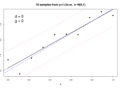
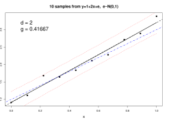
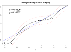
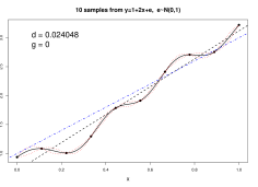
Figure 1 shows two interesting samples from (6). Also plotted are the generating line (dot-dashed), the maximum likelihood (ML) linear model ($\hat{\mbox{\boldmath$\beta$}}$) line (dashed), the predictive mean surface of the ML GP, maximized over range $d$, i.e., the one–vector $\mathbf{d}$, nugget $g$, and $[\sigma^{2}|d,g]$ (solid), and its 95% error bars (dotted). The ML values of $d$ and $g$ are also indicated in each plot. The GP likelihoods were evaluated for ML estimates of the regression coefficients $\hat{\mbox{\boldmath$\beta$}}$. Conditioning on $g$ and $d$, the ML variance was computed by solving

$$0\equiv\frac{d}{d\sigma^{2}}\log N_{n}(\mathbf{y}|\mathbf{F}\hat{\mbox{\boldmath$\beta$}},\sigma^{2}\mathbf{K})=-\frac{n}{\sigma^{2}}+\frac{(\mathbf{y}-\mathbf{F}\hat{\mbox{\boldmath$\beta$}})^{\top}\mathbf{K}^{-1}(\mathbf{y}-\mathbf{F}\hat{\mbox{\boldmath$\beta$}})}{(\sigma^{2})^{2}}.$$

This gave an MLE with the form $\hat{\sigma}^{2}=(\mathbf{y}-\mathbf{F}\hat{\mbox{\boldmath$\beta$}})^{\top}\mathbf{K}^{-1}(\mathbf{y}-\mathbf{F}\hat{\mbox{\boldmath$\beta$}})/n$. For the linear model the likelihood was evaluated as $P(\mathbf{y})=N_{10}(\mathbf{F}\hat{\mbox{\boldmath$\beta$}},\hat{\sigma}^{2}\mathbf{I})$, and for the GP as $P(\mathbf{y}|d,g)=N_{10}\left[\mathbf{F}\hat{\mbox{\boldmath$\beta$}},\hat{\sigma}^{2}\mathbf{K}_{\{d,g\}}\right]$, where $\mathbf{K}_{\{d,g\}}$ is the covariance matrix generated using $K(\cdot,\cdot)=K^{*}(\cdot,\cdot|d)+g\delta_{\cdot,\cdot}$ for $K^{*}(\cdot,\cdot|d)$ from the power family with range parameter $d$.

Figure 1: Two simulations (rows) from $y_{i}=1+2x_{i}+\epsilon_{i},\;\epsilon_{i}\sim N(0,1)$. Left column shows GP fit (solid) with 95% error bars (dotted), maximum likelihood $\hat{\mbox{\boldmath$\beta$}}$ (dashed), and generating linear model ($\mbox{\boldmath$\beta$}=(1,2)$) (dot-dashed). Right column shows GP$(d,g)$ likelihood surfaces, with each curve representing a different value of the nugget $g$. The (maximum) likelihood $(\hat{\mbox{\boldmath$\beta$}})$ of the linear model is indicated by the solid horizontal line.

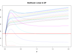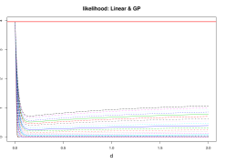
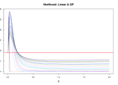
Both samples and fits plotted in Figure 1 have linear looking predictive surfaces, but only for the one in the top row does the linear model have the maximum likelihood. Though the predictive surface in the bottom-left panel could be mistaken as “linear”, it was indeed generated from a GP with large range parameter ($d=2$) and modest nugget setting ($g$) as this parameterization had higher likelihood than the linear model. The right column of Figure 1 shows likelihood surfaces corresponding to the samples in the left column. Each curve corresponds to a different setting of the nugget, $g$. Also shown is the likelihood value of the MLE $\hat{\mbox{\boldmath$\beta$}}$ of the linear model (solid horizontal line). The likelihood surfaces for each sample look drastically different. In the top sample the LLM ($d=0$) uniformly dominates all other GP parameterizations. Contrast this with the likelihood of the second sample. There, the resulting predictive surface looks linear, but the likelihood of the LLM is comparatively low.

Figure 2: Likelihoods as the nugget gets large for single sample of size $n=100$ from Eq. (6). The $x$-axis is $(\log g)$, the range is fixed at $d=1$; the likelihood of the LLM ($d=0$) is shown for comparison.

Figure 2 illustrates the other LLM parameterization by showing how, as the nugget $g$ increases, the likelihood of the GP approaches that of the linear model for a sample of size $n=100$ from (6) with $d$ fixed to one. Observe that the nugget must be quite large relative to the actual variability in the data before the likelihoods of the GP and LLM become comparable.

Figure 3: GP$(d,g)$ fits (left) and likelihood surfaces (right) for two of samples of the LM (6).

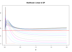Most simulations from (6) gave predictive surfaces like the upper left of Figure 1 and corresponding likelihoods like the upper-right. But this is not always the case. Occasionally a simulation would give high likelihood to GP parameterizations if the sample was slowly waving. This is not uncommon for small sample sizes such as $n=10$. For example, consider those shown in Figure 3. Waviness becomes less likely as the sample size $n$ grows.

Summary:
Min	1.000
1st Qu.	1.000
Median	1.141
Mean	19.160
3rd Qu.	2.619
Max	9419.0

Figure 4: Histogram of the ratio of the maximum likelihood GP parameterization over the likelihood of the limiting linear model with full summary statistics. For visual clarity, the upper tail of the histogram is not shown.

Figure 4 summarizes the ratio of the ML GP parameterization over the ML LM based on 1000 simulations of ten evenly spaced random draws from (6). A likelihood ratio of one means that the LM was best for a particular sample. The 90%-quantile histogram and summary statistics in Figure 4 show that the GP is seldom much better than the LM. For some samples the ratio can be really large ($>9000$) in favor of the GP, but more than two-thirds of the ratios are close to one—approximately 1/3 (362) were exactly one but 2/3 (616) had ratios less than 1.5. This means that the posterior inference for borderline linear data is likely to depend heavily the prior specification of $K(\cdot,\cdot)$.

For some of the smaller nugget values, in particular $g=0$, and larger range settings $d$, the likelihoods for the GP could not be computed because the corresponding covariance matrices were numerically singular, and could not be decomposed. This illustrates a phenomenon noted by Neal (1997) who advocates that a non-zero nugget (or jitter) should be included in the model to increase numerical stability. Numerical instabilities may also be avoided by allowing $p_{i}<2$ in (2), by using the Matérn family of correlation functions (see Section 6), or by simply using an LM where appropriate.

3.1.2 GP posteriors on linear data

Suppose that rather than examining the multivariate normal likelihoods of the linear and GP model, using the ML $\hat{\mbox{\boldmath$\beta$}}$ and $\hat{\sigma}^{2}$ values, the marginalized posterior $p(\mathbf{K}|\mathbf{y},\mbox{\boldmath$\beta$}_{0},\tau^{2},\mathbf{W})$ of Eq. (4) was used, which integrates out $\beta$ and $\sigma^{2}$. Using (4) requires specification of the prior $p(\mathbf{K})$, which for the power family means specifying $p(d,g)$. Alternatively, one could consider dropping the $p(d,g)$ term from (4) and look solely at the marginalized likelihood. However, in light of the arguments above, there is reason to believe that the prior specification will carry significant weight.

If it is suspected that the data might be linear, this bias should be somehow encoded in the prior. This is a non-trivial task, given the nature of the GP parameterizations which encode the LLM. Pushing $d$ towards zero is problematic because small non-zero $d$ causes the predictive surface to be quite wiggly—certainly far from linear. Deciding how small the range parameter ($d$) should be before treating it as zero—as in Stochastic Search Variable Selection (SSVS) of George and McCulloch, (1993), or Chapter 12 of Gilks et al., (1996)—while still allowing a GP to fit truly non-linear data is no simple task. The large nugget approach is also out of the question because putting increasing prior density on a parameter as it gets large is impossible. Rescaling the responses might work, but constructing the prior would be nontrivial. Moreover, such an approach would preclude its use in many applications, particularly for adaptive sampling or sequential design of experiments when one hopes to learn about the range of responses, and/or search for extrema.

However, we have seen that for a continuum of large $d$ values (say $d>0.5$ on the unit interval) the predictive surface is practically linear. Consider a mixture of gammas prior for $d$:

$$p(d,g) =p(d)p(g)=p(g)[G(d|\alpha=1,\beta=20)+G(d|\alpha=10,\beta=10)]/2.$$ (7)

It gives roughly equal mass to small $d$ (mean $1/20$) representing a population of GP parameterizations for wavy surfaces, and a separate population for those which are quite smooth or approximately linear. Figure 8 depicts $p(d)$ via a histogram, ignoring $p(g)$ which is usually taken to be a simple exponential distribution. Alternatively, one could encode the prior as $p(d,g)=p(d|g)p(g)$ and then use a reference prior (Berger et al.,, 2001) for $p(d|g)$. We chose the more deliberate, independent, specification in order to encode our prior belief that there are essentially two kinds of processes: wavy (small $d$) and smooth (large $d$). Observe that $d=0$ is “closer” to the wavy parameterizations—in fact it lies at the limit of extreme waviness. We argue, however, that extreme smoothness may not only be a more intuitive depiction of linearity, but that large $d$-values (though further away) serve as a better platform from which to jump to the LLM.

Evaluation of the marginalized posterior (4) requires settings for the prior mean coefficients $\mbox{\boldmath$\beta$}_{0}$, covariance $\tau^{2}\mathbf{W}$, and hierarchical specifications $(\alpha_{\sigma},\gamma_{\sigma})$ for $\sigma^{2}$. For now, these parameter settings are fixed to those which were known to generate the data.

Figure 5: Top row shows the GP$(d,g)$ fits; Middle row shows likelihoods and bottom row shows the integrated posterior distribution for range ($d$, x-axis) and nugget ($g$, lines) settings for three samples, one per each column. Note that s2 $\equiv\hat{\sigma}^{2}$ in the top row legend(s).

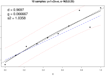
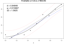
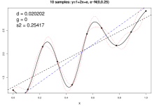
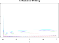
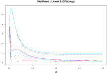
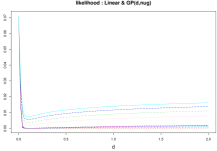
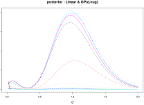
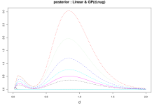
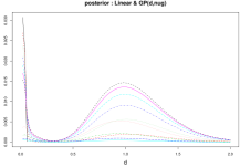
Figure 5 shows three samples from the linear model (6) along with likelihood and posterior surfaces. Occasionally the likelihood and posterior lines suddenly stop due to a numerically unstable parameterization (Neal,, 1997). The GP fits shown in the top row of the figure are based on the maximum a posteriori (MAP) estimates of $d$, $g$, and $\sigma^{2}$. The posteriors in the bottom row clearly show the influence of the prior. Nevertheless, the posterior density for large $d$-values is disproportionately high relative to the prior. Large $d$-values represent at least 90% of the cumulative posterior distribution. Samples from these posteriors would yield mostly linear predictive surfaces. The last sample is particularly interesting as well as being the most representative. Here, the LLM $(d=0)$ is the MAP GP parameterization, and uniformly dominates all other parameterizations in posterior density. Still, the cumulative posterior density favors large $d$-values, thus favoring linear “looking” predictive surfaces over the actual (limiting) linear parameterization.

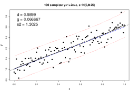
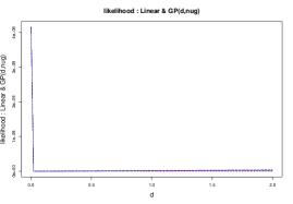
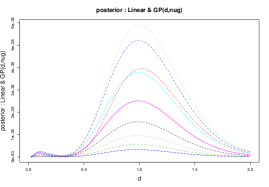
Figure 6 (top left) shows a representative MAP GP fit for a sample of size $n=100$ from (6). Since larger samples have a lower probability of coming out wavy, the likelihood of the LLM (on the right) is much higher than other GP parameterizations, though it is severely peaked. Small, nonzero, $d$-values have extremely low likelihood. By contrast, the posterior in the bottom panel puts high density on large $d$-values. The MAP predictive surface (top left) has a very small, but noticeable, amount of curvature.

Figure 6: Top-left shows the GP$(d,g)$ fit with a sample of size $n=100$; top-right shows the likelihood and bottom-right shows the integrated posterior for range ($d$, x-axis) and nugget ($g$, lines) settings.

Ideally, linear looking predictive surfaces should not have to bear the computational burden implied by full–fledged GPs. But since the LLM $(d=0)$ is a point-mass (which is the only parameterization that actually gives an identity covariance matrix), it has zero probability under the posterior. It would never be sampled in an MCMC, even when it did happen to be the MAP estimate.

3.1.3 GP posteriors and likelihoods on non-linear data

For completeness, Figure 7 and shows fits, likelihoods, and posteriors on non-linear data. The first column of Figure 7 corresponds to a sample with quadratic mean, and each successive column corresponds to a sample which is increasingly wavy.

Figure 7: Top row shows the GP$(d,g)$ fits; Middle row shows likelihoods and bottom row shows the integrated posterior distribution for range ($d$, x-axis) and nugget ($g$, lines) settings for four samples, one per each column .As the samples become less linear the $d$-axis (x-axis) shrinks in order to focus in on the mode.

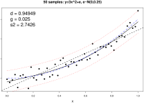
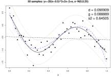
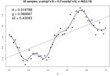
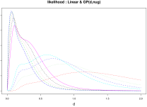
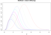
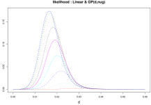
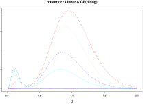
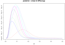
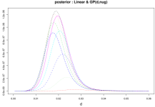
Each sample is of size $n=50$. The shape of the prior loses its influence as the data become more non-linear. Although in all three cases the MLEs do not correspond to the MAP estimates, the corresponding ML and MAP predictive surfaces look remarkably similar (not shown). This is probably due to the fact that the posterior integrates out $\beta$ and $\sigma^{2}$, whereas the likelihoods were computed with point estimates of these parameters.

4 Model selection prior

Figure 8: Histogram of the mixture of gammas prior $p(d)$ as given in Eq. (7), with the prior distribution for the boolean ($b$) superimposed on $p(d)$ from Eq.(8) using $(\gamma,\theta_{1},\theta_{2})=(10,0.2,0.95)$ .

With the ideas outlined above, we set out to construct a prior for the “mixture” of the GP with its LLM by focusing on large range parameters rather than $\mathbf{d}=\mathbf{0}$ or $g\rightarrow\infty$. The key idea is an augmentation of the parameter space by $m_{X}$ latent indicator variables $\mathbf{b}=\{b\}_{i=1}^{m_{X}}\in\{0,1\}^{m_{X}}$. The boolean $b_{i}$ is intended to select either the GP ($b_{i}=1$) or its LLM for the $i^{\mbox{\tiny th}}$ dimension. The actual range parameter used by the correlation function is multiplied by $\mathbf{b}$: e.g. $K^{*}(\cdot,\cdot|\mathbf{b}\mathbf{d})$. To encode our preference that GPs with larger range parameters should be more likely to “jump” to the LLM, the prior on $b_{i}$ is specified as a function of the range parameter $d_{i}$: $p(b_{i},d_{i})=p(b_{i}|d_{i})p(d_{i})$.

Probability mass functions which increase as a function of $d_{i}$, e.g.,

$$p_{\gamma,\theta_{1},\theta_{2}}(b_{i}=0|d_{i})=\theta_{1}+(\theta_{2}-\theta_{1})/(1+\exp\{-\gamma(d_{i}-0.5)\})$$ (8)

with $0<\gamma$ and $0\leq\theta_{1}\leq\theta_{2}<1$, can encode such a preference by calling for the exclusion of dimensions $i$ with with large $d_{i}$ when constructing $\mathbf{K}$. Thus $b_{i}$ determines whether the GP or the LLM is in charge of the marginal process in the $i^{\mbox{\tiny th}}$ dimension. Accordingly, $\theta_{1}$ and $\theta_{2}$ represent minimum and maximum probabilities of jumping to the LLM, while $\gamma$ governs the rate at which $p(b_{i}=0|d_{i})$ grows to $\theta_{2}$ as $d_{i}$ increases. Figure 8 plots $p(b_{i}=0|d_{i})$ for $(\gamma,\theta_{1},\theta_{2})=(10,0.2,0.95)$ superimposed on the mixture of gammas prior $p(d_{i})$ from (7). The $\theta_{2}$ parameter is taken to be strictly less than one so as not to preclude a GP which models a genuinely nonlinear surface using an uncommonly large range setting.

The implied prior probability of the full $m_{X}$-dimensional LLM is

$$p(\mbox{linear model})=\prod_{i=1}^{m_{X}}p(b_{i}=0|d_{i})=\prod_{i=1}^{m_{X}}\left[\theta_{1}+\frac{\theta_{2}-\theta_{1}}{1+\exp\{-\gamma(d_{i}-0.5)\}}\right].$$ (9)

Observe that the resulting process is still a GP if any of the booleans $b_{i}$ are one. The primary computational advantage associated with the LLM is foregone unless all of the $b_{i}$’s are zero. However, the intermediate result offers an improvement in numerical stability in addition to describing a unique transitionary model lying somewhere between the GP and the LLM. Specifically, it allows for the implementation of semiparametric stochastic processes like $Z(\mathbf{x})=\mbox{\boldmath$\beta$}f(\mathbf{x})+\varepsilon(\tilde{\mathbf{x}})$, representing a piecemeal spatial extension of a simple linear model. The first part ($\mbox{\boldmath$\beta$}f(\mathbf{x})$) of the process is linear in some known function of the full set of covariates $\mathbf{x}=\{x_{i}\}_{i=1}^{m_{X}}$, and $\varepsilon(\cdot)$ is a spatial random process (e.g., a GP) which acts on a subset of the covariates $\tilde{\mathbf{x}}$. Such models are commonplace in the statistics community (Dey et al.,, 1998). Traditionally, $\tilde{\mathbf{x}}$ is determined and fixed a priori. The separable boolean prior in (8) implements an adaptively semiparametric process where the subset $\tilde{\mathbf{x}}=\{x_{i}:b_{i}=1,i=1,\dots,m_{X}\}$ is given a prior distribution, instead of being fixed.

So even if the computational advantage of the LLM is not present because some $b_{i}\neq 0$ we still have that any $b_{i}=0$ setting releases us from the burden of sampling the corresponding $d_{i}$. It also imparts on us the knowledge that the response has (at best) a linear relationship with the $i^{\mbox{\tiny th}}$ covariate. This approach may also increase the scope for analysis of higher dimensional datasets, where data sparseness in higher dimensions (the “curse of dimensionality”) can be ameliorated by using linear models in most dimensions and GP models only in the dimensions where they will have the most effect, thus reducing the dimension of the GP model space.

Note that if an isotropic correlation function is used, which has only a single range parameter, then only one boolean $b$ is needed, and the product can be dropped from (9). In this case, however, the advantage of being able to detect linearity, marginally, in each dimension is lost.

4.1 Prediction

Prediction under the LLM parameterization of the GP model (5) can be simplified when all of the booleans are zero, whence it is known that $\mathbf{K}=(1+g)\mathbf{I}$. A characteristic of the standard linear model is that all input configurations $(\mathbf{x})$ are treated as independent conditional on knowing $\beta$. This additionally implies that in (5) the terms $k(\mathbf{x})$ and $K(\mathbf{x},\mathbf{x}_{j})$ are zero for all $\mathbf{x}$. Thus, the predicted value of $y$ at $\mathbf{x}$ is normally distributed with mean $\hat{y}(\mathbf{x})=\mathbf{f}^{\top}(\mathbf{x})\tilde{\mbox{\boldmath$\beta$}}$ and variance

$$\sigma^{2}[1+\tau^{2}\mathbf{f}^{\top}(\mathbf{x})\mathbf{W}\mathbf{f}(\mathbf{x})-\tau^{2}\mathbf{f}^{\top}(\mathbf{x})\mathbf{W}\mathbf{F}^{\top}((1+g)\mathbf{I}+\tau^{2}\mathbf{F}\mathbf{W}\mathbf{F}^{\top})^{-1}\mathbf{F}\mathbf{W}\mathbf{f}(\mathbf{x})\tau^{2}].$$

It is helpful to re-write the above expression for the variance as

$$\hat{\sigma}(\mathbf{x})^{2} =\sigma^{2}[1+\tau^{2}\mathbf{f}^{\top}(\mathbf{x})\mathbf{W}\mathbf{f}(\mathbf{x})]$$ (10)

$$-\sigma^{2}\left[1+\tau^{2}\mathbf{f}^{\top}(\mathbf{x})\mathbf{W}\mathbf{f}(\mathbf{x})-\frac{\tau^{2}}{1+g}\mathbf{f}^{\top}(\mathbf{x})\mathbf{W}\mathbf{F}^{\top}\left(\mathbf{I}+\frac{\tau^{2}}{1+g}\mathbf{F}\mathbf{W}\mathbf{F}^{\top}\right)^{-1}\mathbf{F}\mathbf{W}\mathbf{f}(\mathbf{x})\tau^{2}\right].$$

A matrix inversion lemma called the Woodbury formula (Golub and Van Loan,, 1996, pp. 51) or the Sherman–Morrison–Woodbury formula (Bernstein,, 2005, pp. 67) states that for $(\mathbf{I}+\mathbf{V}^{\top}\mathbf{A}\mathbf{V})$ non-singular $(\mathbf{A}^{-1}+\mathbf{V}\mathbf{V}^{\top})^{-1}=\mathbf{A}-(\mathbf{A}\mathbf{V})(\mathbf{I}+\mathbf{V}^{\top}\mathbf{A}\mathbf{V})^{-1}\mathbf{V}^{\top}\mathbf{A}.$ Taking $\mathbf{V}\equiv\mathbf{F}^{\top}(1+g)^{-\frac{1}{2}}$ and $\mathbf{A}\equiv\tau^{2}\mathbf{W}$ in (10) gives

$$\hat{\sigma}(\mathbf{x})^{2}=\sigma^{2}\left[1+\mathbf{f}^{\top}(\mathbf{x})\left(\frac{\mathbf{W}^{-1}}{\tau^{2}}+\frac{\mathbf{F}^{\top}\mathbf{F}}{1+g}\right)^{-1}\mathbf{f}(\mathbf{x})\right].$$ (11)

Eq. (11) is not only a simplification of the predictive variance given in (5), but it should look familiar. Writing $\mathbf{V}_{\tilde{\beta}}$ with $\mathbf{K}^{-1}=\mathbf{I}/(1+g)$ in (3) gives

$$\mathbf{V}_{\tilde{\beta}}=\left(\frac{\mathbf{W}^{-1}}{\tau^{2}}+\frac{\mathbf{F}^{\top}\mathbf{F}}{1+g}\right)^{-1}\;\;\;\;\;\mbox{and then:}\;\;\;\;\;\hat{\sigma}(\mathbf{x})^{2}=\sigma^{2}\left[1+\mathbf{f}^{\top}(\mathbf{x})\mathbf{V}_{\tilde{\beta}}\mathbf{f}(\mathbf{x})\right].$$ (12)

This is just the usual posterior predictive density at $\mathbf{x}$ under the standard linear model: $y(\mathbf{x})~{}\sim~{}N[\mathbf{f}^{\top}(\mathbf{x})\tilde{\mbox{\boldmath$\beta$}},\sigma^{2}(1+\mathbf{f}^{\top}(\mathbf{x})\mathbf{V}_{\tilde{\beta}}\mathbf{f}(\mathbf{x}))]$. This means that we have a choice when it comes to obtaining samples from the posterior predictive distribution under the LLM. We prefer (12) over (5) because the latter involves inverting the $n\times n$ matrix $\mathbf{I}+\tau^{2}\mathbf{F}\mathbf{W}\mathbf{F}^{\top}/(1+g)$, whereas the former only requires the inversion of an $m\times m$ matrix. Of course, if any of the booleans are non-zero, then GP prediction must proceed as usual, following Eq. (5).

GP fits to typical nonlinear response surfaces may seldom achieve $b_{i}=0$ for all $i$. However, the following section illustrates how treed partitioning can dramatically increase the probability of jumping to the LLM parameterization (in at least part of the input space) where the more thrifty predictive equations (12) may be exploited.

5 Implementation, results, and comparisons

Here, the GP with jumps to the LLM (hereafter GP LLM) is illustrated on synthetic and real data. This work grew out of research focused on extending the reach of the treed GP model presented by Gramacy and Lee, (2008), whereby the data are recursively partitioned and a separate GP is fit in each partition. Thus most of our experiments are in this context, though in Section 5.3 we demonstrate an example without treed partitioning. Partition models are an ideal setting for evaluating the utility of the GP LLM, as linearity can be extracted in large areas of the input space. The result is a uniquely tractable nonstationary semiparametric spatial model.

A separable correlation function is used throughout this section for brevity and consistency, even though in some cases the process which generated the data is clearly isotropic. Proposals for the booleans $\mathbf{b}$ are drawn from the prior, conditional on $\mathbf{d}$, and accepted and rejected on the basis of the constructed covariance matrix $\mathbf{K}$. The same prior parameterizations are used for all experiments unless otherwise noted, the idea being to develop a method that works “right out of the box” as much as possible.

5.1 Synthetic exponential data

Consider the 2-d input space $[-2,6]\times[-2,6]$ in which the true response is given by $Y(\mathbf{x})=x_{1}\exp(-x_{1}^{2}-x_{2}^{2})+\epsilon$, where $\epsilon\sim N(0,\sigma=0.001)$.

Figure 9: Left: exponential data GP LLM fit. Right: histogram of the areas under the LLM.

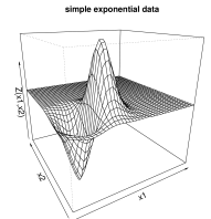
Figure 9 summarizes the consequences of estimation and prediction with the treed GP LLM for a $n=200$ random sub-sample of this data from a regular grid of size 441. The partitioning structure of the treed GP LLM first splits the region into two halves, one of which can be fit linearly. It then recursively partitions the half with the action into a piece which requires a GP and another piece which is also linear. The left pane shows a mean predictive surface wherein the LLM was used over 66% of the domain (on average) which was obtained in less than ten seconds on a 1.8 GHz Athalon. The right pane shows a histogram of the areas of the domain under the LLM over 20-fold repeated experiments. The four modes of the histogram clump around 0%, 25%, 50%, and 75% showing that most often the obvious three–quarters of the space is under the LLM, although sometimes one of the two partitions will use a very smooth GP. The treed GP LLM was 40% faster than the treed GP alone when combining estimation and sampling from the posterior predictive distributions at the remaining $n^{\prime}=241$ points from the grid.

5.2 Motorcycle Data

The Motorcycle Accident Dataset (Silverman,, 1985) is a classic for illustrating nonstationary models. It samples the acceleration force on the head of a motorcycle rider as a function of time in the first moments after an impact. Figure 10 shows the data and a fit using the treed GP LLM. The plot shows the mean predictive surface with 90% quantile error bars, along with a typical partition. On average, 29% of the domain was under the LLM, split between the left low–noise region (before impact) and the noisier rightmost region.

Figure 10: Motorcycle Data fit by treed GP LLM.

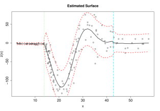
Rasmussen and Ghahramani, (2002) analyzed this data using a Dirichlet process mixture of Gaussian process (DPGP) experts which reportedly took one hour on a 1 GHz Pentium. Such times are typical of inference under nonstationary models because of the computational effort required to construct and invert large covariance matrices. In contrast, the treed GP LLM fits this dataset with comparable accuracy but in less than one minute on a 1.8 GHz Athalon.

We identify three things which make the treed GP LLM so fast relative to most nonstationary spatial models. (1) Partitioning fits models to less data, yielding smaller matrices to invert. (2) Jumps to the LLM mean fewer inversions all together. (3) MCMC mixes better because under the LLM the parameters $\mathbf{d}$ and $g$ are out of the picture and all sampling can be performed via Gibbs steps.

5.3 Friedman data

This Friedman dataset is the first one of a suite that was used to illustrate MARS (Multivariate Adaptive Regression Splines) (Friedman,, 1991). There are 10 covariates in the data ($\mathbf{x}=\{x_{1},x_{2},\dots,x_{10}\}$), but the function that describes the responses ($Y$), observed with standard Normal noise,

$$E(Y|\mathbf{x})=\mu=10\sin(\pi x_{1}x_{2})+20(x_{3}-0.5)^{2}+10x_{4}+5x_{5}$$ (13)

depends only on $\{x_{1},\dots,x_{5}\}$, thus combining nonlinear, linear, and irrelevant effects. We make comparisons on this data to results provided for several other models in recent literature. Chipman et al., (2002) used this data to compare their treed LM algorithm to four other methods of varying parameterization: linear regression, greedy tree, MARS, and neural networks. The statistic they use for comparison is root mean–squared error, $\mbox{RMSE}=\sqrt{\sum_{i=1}^{n}(\mu_{i}-\hat{Y}_{i})^{2}/n}$, where $\hat{Y}_{i}$ is the model–predicted response for input $\mathbf{x}_{i}$. The $\mathbf{x}$’s are randomly distributed on the unit interval. RMSE’s are gathered for fifty repeated simulations of size $n=100$ from (13). Chipman et al. provide a nice collection of boxplots showing the results. However, they do not provide any numerical results, so we have extracted some key numbers from their plots and refer the reader to their paper for the full results.

We duplicated the experiment using both a stationary GP and our GP LLM. For this dataset, we use a single model, not a treed model, as the function is essentially stationary in the spatial statistical sense (so if we were to try to fit a treed GP, it would keep all of the data in a single partition). Linearizing boolean prior parameters $(\gamma,\theta_{1},\theta_{2})=(10,0.2,0.9)$ were used, which gave the LLM a relatively low prior probability of 0.35, for large range parameters $d_{i}$. The RMSEs that we obtained for the stationary GP and the GP LLM are summarized in the table below.

	Min	1st Qu.	Median	Mean	3rd Qu.	Max
GP LLM	0.4341	0.5743	0.6233	0.6258	0.6707	0.7891
GP	0.8196	0.8835	0.9131	0.9232	0.9710	1.0440
Linear	1.710	2.165	2.291	2.325	2.500	2.794

Results on the linear model are reported for calibration purposes, and can be seen to be essentially the same as those reported by Chipman et al. RMSEs for the GP LLM are on average significantly better than all of those reported for the above methods, with lower variance. For example, the best mean RMSE shown in the boxplot is $\approx 0.9$. That is 1.4 times higher than the worst one we obtained for GP LLM. Further comparison to the boxplots provided by Chipman et al. shows that the GP LLM is the clear winner. It is also clear that jumping to a linear model in the relevant dimensions provides a more stable fit that gives improved predictive performance relative to a full (stationary) GP.

In fitting the model, the Markov Chain quickly keyed in on the fact that only the first three covariates contribute nonlinearly. After burn–in, the booleans $\mathbf{b}$ almost never deviated from $(1,1,1,0,0,0,0,0,0,0)$. From the following table summarizing the posterior for the linear regression coefficients ($\beta$) we can see that the coefficients for $x_{4}$ and $x_{5}$ (between double-bars) were estimated accurately, and that the model correctly determined that $\{x_{6},\dots x_{10}\}$ were irrelevant (i.e. not included in the GP, and had $\beta$’s close to zero).

		$x_{4}$	$x_{5}$	$x_{6}$	$x_{7}$	$x_{8}$	$x_{9}$	$x_{10}$
	5% Qu.	8.40	2.60	-1.23	-0.89	-1.82	-0.60	- 0.91
$\beta$	Mean	9.75	4.59	-0.190	0.049	-0.612	0.326	0.066
	95% Qu.	10.99	9.98	0.92	1.00	0.68	1.21	1.02

For a final comparison we consider a Support Vector Machine (SVM) method (Drucker et al.,, 1996) illustrated on this data and compared to Bagging (Breiman,, 1996). We note that the SVM method required cross-validation (CV) to set some of its parameters. In the comparison, 100 randomized training sets of size $n=200$ were used, and RMSEs were collected for a (single) test set of size $n^{\prime}=1000$. An average MSE of 0.67 is reported, showing the SVM to be uniformly better the Bagging method with an MSE of 2.26. We repeated the experiment for the GP LLM (which requires no CV!), and obtained an average MSE of 0.293, which is 2.28 times better than the SVM, and 7.71 times better than Bagging.

5.4 Boston housing data

A commonly used dataset for validating multivariate models is the Boston Housing Data (Harrison and Rubinfeld,, 1978), which contains 506 responses over 13 covariates. Chipman et al., (2002) showed that their (Bayesian) treed LM gave lower RMSEs, on average, compared to a number of popular techniques (the same ones listed in the previous section). Here we employed a treed GP LLM, which is a generalization of their treed LM, retaining the original treed LM as an accessible special case. Though computationally more intensive than the treed LM, the treed GP LLM gives impressive results. To mitigate some of the computational demands, the LLM can be used to initialize the Markov Chain by breaking the larger dataset into smaller partitions. Before treed GP burn–in begins, the model is fit using only the faster (limiting) treed LM model. Once the treed partitioning has stabilized, this fit is taken as the starting value for a full MCMC exploration of the posterior for the treed GP LLM. This initialization process allows us to fit GPs on smaller segments of the data, reducing the size of matrices that need to be inverted and greatly reducing computation time. For the Boston Housing data we use $(\gamma,\theta_{1},\theta_{2})=(10,0.2,0.95)$, which gives the LLM a prior probability of $0.95^{13}\approx 0.51$, when the $d_{i}$’s are large.

Experiments in the Bayesian treed LM paper (Chipman et al.,, 2002) consist of calculating RMSEs via 10-fold CV. The data are randomly partitioned into 10 groups, iteratively trained on 9/10 of the data, and tested on the remaining 1/10. This is repeated for 20 random partitions, and boxplots are shown. Note that the logarithm of the response is used and that CV is only used to assess predictive error, not to tune parameters. Samples are gathered from the posterior predictive distribution of the treed LM for six parameterizations using 20 restarts of 4000 iterations. This seems excessive, but we followed suit for the treed GP LLM in order to obtain a fair comparison. Our “boxplot” for training and testing RMSEs are summarized in the table below. As before, linear regression (on the log responses) is used for calibration.

		Min	1st Qu.	Median	Mean	3rd Qu.	Max
train	GP LLM	0.0701	0.0716	0.0724	0.0728	0.0730	0.0818
	Linear	0.1868	0.1869	0.1869	0.1869	0.1869	0.1870
test	GP LLM	0.1321	0.1327	0.1346	0.1346	0.1356	0.1389
	Linear	0.1926	0.1945	0.1950	0.1950	0.1953	0.1982

Notice that the RMSEs for the linear model have extremely low variability. This is similar to the results provided by Chipman et al. and was a key factor in determining that our experiment was well–calibrated. Upon comparison of the above numbers with the boxplots in Chipman et al., it can readily be seen that the treed GP LLM is leaps and bounds better than the treed LM, and all of the other methods in the study. Our worst training RMSE is almost two times lower than the best ones from the boxplot. All of our testing RMSEs are lower than the lowest ones from the boxplot, and our median RMSE (0.1346) is 1.26 times lower than the lowest median RMSE ($\approx 0.17$) from the boxplot.

More recently, Chu et al., (2004) performed a similar experiment (see Table V), but instead of 10-fold CV, they randomly partitioned the data 100 times into training/test sets of size 481/25 and reported average MSEs on the un-transformed responses. They compare their Bayesian SVM regression algorithm (BSVR) to other high-powered techniques like Ridge Regression, Relevance Vector Machine, GPs, etc., with and without ARD (automatic relevance determination—essentially, a separable covariance function). Repeating their experiment for the treed GP LLM gave an average MSE of 6.96 compared to that of 6.99 for the BSVR with ARD, making the two algorithms by far the best in the comparison. However, without ARD the MSE of BSVR was 12.34, 1.77 times higher than the treed GP LLM, and the worst in the comparison. The reported results for a GP with (8.32) and without (9.13) ARD showed the same effect, but to a lesser degree. Perhaps not surprisingly, the average MSEs do not tell the whole story. The 1st, median, and 3rd quartile MSEs we obtained for the treed GP LLM were 3.72, 5.32 and 8.48 respectively, showing that its distribution had a heavy right–hand tail. We take this as an indication that several responses in the data are either misleading, noisy, or otherwise very hard to predict.

6 Conclusions

Gaussian processes are a flexible modeling tool which can be an overkill for many applications. We have shown how its limiting linear model can be both useful and accessible in terms of Bayesian posterior estimation, and prediction. The benefits include speed, parsimony, and a relatively straightforward implementation of a semiparametric model. When combined with treed partitioning the GP LLM extends the treed LM, resulting in a uniquely nonstationary, tractable, and highly accurate regression tool.

We have focused on the separable power family of correlation functions, but the methodology is by no means restricted to this family. All that is required is that the relevant family have a range parameter (like $\mathbf{d}$) that yields the limiting (scaled) identity covariance matrix characterizing the LLM (like $\mathbf{d}\rightarrow 0$). For example, allowing a power $0<p_{i}\neq 2$ in the power family of Eq. (2) is straightforward. The separable Matérn family also has the desired property:

$$K(\mathbf{x}_{j},\mathbf{x}_{k}|\rho,\phi,\mathbf{d})=\prod_{i=1}^{m_{X}}\frac{\pi^{1/2}\phi d_{i}^{2\rho}}{2^{\rho-1}\Gamma(\rho+1/2)}(||x_{ij}-x_{ik}||/d_{i})^{\rho}\mathcal{K}_{\rho}(||x_{ij}-x_{ik}||/d_{i}),$$

where $\mathcal{K}_{\rho}$ is a modified Bessel function of the second kind. Unlike the power family, the isotropic Matérn family does not arise as a special case where $d_{i}=d$, for $i=1,\dots,m_{X}$, but, as mentioned in Section 4, the LLM methodology remains similarly applicable when there is only one range parameter.

One obvious extension of this work is to allow a larger class of “simple” models for the mean function of the process, such as higher-order polynomials or interactions between linear terms. Choosing among simpler models can be done straightforwardly within the Bayesian framework (George and McCulloch,, 1993; Geweke,, 1996; Joseph et al.,, 2008). Such an extension would likely allow more frequent selection of the simpler model, reducing the need for the GP. However, the clear understanding of what limiting cases lead to jumping from a GP to a linear model, as well as how to construct a set of booleans and their priors, would be lost in moving beyond linear models. Over a local region, a quadratic function would be well–approximated by a GP with a range parameter that could be neither very small nor large. Thus the approach contained herein would need further thought to efficiently extend it. There is also the tradeoff of the extra computing resources needed to test a larger set of models, whereas linear models can be worked directly into the current model fitting (via the auxiliary booleans), and do not require separate model selection steps.

We believe that a large contribution of the GP LLM will be in the domain of sequential design of computer experiments (Gramacy and Lee,, 2008) which was the inspiration for much of the work presented here. Empirical evidence suggests that many computer experiments are nearly linear. That is, either the response is linear in most of its input dimensions, or the process is entirely linear in a subset of the input domain. Supremely relevant, but largely ignored in this paper, is that the Bayesian treed GP LLM provides a full posterior predictive distribution (particularly a nonstationary and thus region–specific estimate of predictive variance) which can be used towards active learning in the input domain. Exploitation of these characteristics should lead to an efficient framework for the adaptive exploration of computer experiment parameter spaces.

References

- Berger et al., (2001) Berger, J. O., de Oliveira, V., and Sansó, B. (2001). “Objective Bayesian Analysis of Spatially Correlated Data.” Journal of the American Statistical Association, 96, 456, 1361–1374.
- Bernstein, (2005) Bernstein, D. (2005). Matrix Mathematics. Princeton, NJ: Princeton University Press.
- Breiman, (1996) Breiman, L. (1996). “Bagging Predictors.” Machine Learning, 24, 2, 123–140.
- Calder, (2007) Calder, C. A. (2007). “Dynamic factor process convolution models for multivariate space time data with application to air quality assessment.” Environmental and Ecological Statistics, 14, 229–247.
- Chilés and Delfiner, (1999) Chilés, J. and Delfiner, P. (1999). Geostatistics: Modeling Spatial Uncertainty. John Wiley and Sons, Inc.
- Chipman et al., (1998) Chipman, H., George, E., and McCulloch, R. (1998). “Bayesian CART Model Search (with discussion).” Journal of the American Statistical Association, 93, 935–960.
- Chipman et al., (2002) — (2002). “Bayesian Treed Models.” Machine Learning, 48, 303–324.
- Chu et al., (2004) Chu, W., Keerthi, S. S., and Ong, C. J. (2004). “Bayesian Support Vector Regression using a Unified Loss Function.” IEEE Transactions on Neural Networks, 15(1), 29–44.
- Cressie, (1991) Cressie, N. (1991). Statistics for Spatial Data. John Wiley and Sons, Inc.
- Dey et al., (1998) Dey, D., Müller, P., and Sinha, D. (1998). Practical Nonparametric and Semiparametric Bayesian Statistics. New York, NY, USA: Springer-Verlag New York, Inc.
- Drucker et al., (1996) Drucker, H., Burges, C. J. C., Kaufman, L., Smola, A. J., and Vapnik, V. (1996). “Support Vector Regression Machines.” In Advances in Neural Information Processing Systems, 155–161. MIT Press.
- Friedman, (1991) Friedman, J. H. (1991). “Multivariate Adaptive Regression Splines.” Annals of Statistics, 19, No. 1, 1–67.
- George and McCulloch, (1993) George, E. I. and McCulloch, R. E. (1993). “Variable selection via Gibbs sampling.” Journal of the American Statistical Association, 88, 881–889.
- Geweke, (1996) Geweke, J. (1996). “Variable selection and model comparison in regression.” In In Bayesian Statistics 5, eds. J. Bernardo, J. Berger, A. Dawid, and A. Smith, 609–620. Oxford Press.
- Gilks et al., (1996) Gilks, W., Richardson, S., and Spiegelhalter, D. (1996). Markov Chain Monte Carlo in Practice. London: Chapman & Hall.
- Gilleland and Nychka, (2005) Gilleland, E. and Nychka, D. (2005). “Statistical models for monitoring and regulating ground-level ozone.” Environmetrics, 16, 535–546.
- Golub and Van Loan, (1996) Golub, G. H. and Van Loan, C. F. (1996). Matrix Computations. Baltimore, MD: Johns Hopkins.
- Gramacy, (2007) Gramacy, R. B. (2007). “tgp: An R Package for Bayesian Nonstationary, Semiparametric Nonlinear Regression and Design by Treed Gaussian Process Models.” Journal of Statistical Software, 19, 9.
- Gramacy and Lee, (2008) Gramacy, R. B. and Lee, H. K. H. (2008). “Bayesian treed Gaussian process models with an application to computer modeling.” Journal of the American Statistical Association, to appear.
- Gramacy and Taddy, (2008) Gramacy, R. B. and Taddy, M. A. (2008). tgp: Bayesian treed Gaussian process models. R package version 2.1-2.
- Harrison and Rubinfeld, (1978) Harrison, D. and Rubinfeld, D. L. (1978). “Hedonic Housing Prices and the Demand for Clean Air.” Journal of Environmental Economics and Management, 5, 81–102.
- Joseph et al., (2008) Joseph, V. R., Hung, Y., and Sudjianto, A. (2008). “Blind Kriging: A New Method for Developing Metamodels.” AMSE Journal of Mechanical Design. To appear.
- Kennedy and O’Hagan, (2001) Kennedy, M. and O’Hagan, A. (2001). “Bayesian Calibration of Computer Models (with discussion).” Journal of the Royal Statistical Society, Series B, 63, 425–464.
- Neal, (1997) Neal, R. (1997). “Monte Carlo implementation of Gaussian process models for Bayesian regression and classification”.” Tech. Rep. CRG–TR–97–2, Dept. of Computer Science, University of Toronto.
- Rasmussen and Ghahramani, (2002) Rasmussen, C. and Ghahramani, Z. (2002). “Infinite Mixtures of Gaussian Process Experts.” In Advances in Neural Information Processing Systems, vol. 14, 881–888. MIT Press.
- Santner et al., (2003) Santner, T. J., Williams, B. J., and Notz, W. I. (2003). The Design and Analysis of Computer Experiments. New York, NY: Springer-Verlag.
- R Development Core Team, (2004) R Development Core Team (2004). R: A language and environment for statistical computing. R Foundation for Statistical Computing, Vienna, Aus. ISBN 3-900051-00-3.
- Silverman, (1985) Silverman, B. W. (1985). “Some Aspects of the Spline Smoothing Approach to Non-Parametric Curve Fitting.” Journal of the Royal Statistical Society Series B, 47, 1–52.