Separating Signals from Non-Interfering Backgrounds
using
Probabilistic Event Weightings.
Abstract
A common situation in experimental physics is to have a signal which can not be separated from a non-interfering background through the use of any cut. In this paper, we describe a procedure for determining, on an event-by-event basis, a quality factor (-factor) that a given event originated from the signal distribution. This -factor can then be used as an event weight in subsequent analysis procedures, allowing one to more directly access the true spectrum of the signal.
keywords:
PACS:
29.85.-c , 29.85.Fj, and
1 Introduction
In many physics analyses, one has non-interfering background events which cannot be cleanly separated from the desired signal. This is of particular concern when the problem being studied is multi-dimensional, i.e. there are kinematic correlations in the signal which must be preserved. One typical way to handle these situations is with the side-band subtraction method. Distributions constructed using events outside the signal region are subtracted from those using events inside the signal region to create distributions in which the backgrounds have been removed. While this method can be effective in some situations, implementing it can become problematic if the kinematics of the background region are different than those of the signal or if the problem is sufficiently multi-dimensional such that binning the data is severely limited by statistical uncertainties.
In this paper, we describe a procedure for assigning each event in a data sample a quality factor (-factor) which gives the chance that it originates from the signal sample. This -factor can then be used as an event weight in subsequent analysis procedures to gain access to the signal distribution. For example, the -factors can be used to perform event-based unbinned maximum likelihood fits on the data to extract physical observables. Eliminating the need to bin the data is highly desirable for the case of multi-dimensional problems. We note here that this procedure is not appropriate for situations where there are quantum mechanical interference effects between the signal and background.
2 Quality Factor Determination
Consider a data set composed of total events, each of which is described by coordinates (). The coordinates can be masses, angles, energies, etc. Furthermore, the data set consists of signal and background events. Both the signal and background distributions are functions of the coordinates, and respectively. For this procedure, we need to know a priori the functional dependence (possibly with unknown parameters) of the signal and background distributions in terms of one of the coordinates. We will refer to this coordinate as the reference coordinate and label it .
As an example, consider the case where the reference coordinate is a mass. The functional dependence of the signal, in terms of , might be given by a Gaussian or Breit-Wigner distribution. The background may be well represented by a polynomial. In both cases, there could be unknown parameters (e.g. the width of the Gaussian); these are permitted when using this procedure. No other a priori information is required concerning the dependence of or on any of the other coordinates.
The aim of this procedure is to assign each event a quality factor, or -factor, which gives the chance that it originates from the signal sample. We first need to define a metric for the space spanned by (excluding ). A reasonable choice is to use where is the maximum possible difference between the coordinates of any two events in the sample. Using this metric, the distance between any two events, , is given as
| (1) |
where the sum is over all coordinates except .
For each event, we compute the distance to all other events in the data set, and retain the nearest neighbor events, including the events itself, according to (1). The value of , which varies depending on the analysis, is discussed below. The events are then fit using the unbinned maximum likelihood method to obtain estimators for the parameters, , in the probability distribution function
| (2) |
where and describe the functional dependence on the reference coordinate, , of the signal and background respectively.
The -factor for each event is then calculated as
| (3) |
where is the value of the event’s reference coordinate and are the estimators for the parameters obtained from the event’s fit.
If one wants to bin the data, the signal yield in a bin is obtained as
| (4) |
where is the number of events in the bin. For example, to construct a histogram (of any dimension) of the signal, one would simply weight each event’s contribution by its -factor.
3 Error Estimation
It is also important to extract the uncertainties on the individual -factors so that we can obtain error estimates on measurable quantities. The full covariance matrix obtained from each event’s fit, , can be used to calculate the uncertainty in as
| (5) |
When using these values to obtain errors on the signal yield in any bin, we must consider the fact that the nature of our procedure leads to highly-correlated results for each event and its nearest neighbors; thus, simply adding the values in quadrature would certainly underestimate the true error. The actual degree of correlation of the -factors would depend on the population of the bins. A safe choice is to assume 100% correlation; thus,
| (6) |
which provides an overestimate of the true uncertainty inherent in the procedure.
In addition to the uncertainties associated with the fits, there will also be a purely statistical error associated with the signal yield in each bin, given by Poisson statistics. For large values of , the signal yield obtained using (4), this can be taken to be ; however, for smaller the upper limit is better approximated by [1]. The total uncertainty on the signal yield in any bin is then obtained by adding the fit errors, calculated using (6), in quadrature with the statistical errors discussed above.

4 Example Application
As an example, we will consider the reaction in a single bin, i.e. a single center-of-mass energy and production angle bin (extending the example to avoid binning in production angle, or , is discussed below). The decays to about 90% of the time; thus, we will assume we have a detector which has reconstructed events. Of course, there are production mechanisms other than which can produce this final state and there is no cut which can be performed to separate out events that originated from . Below we will construct a toy-model of this situation by generating Monte Carlo events for both signal, i.e. events, and background, i.e. non- events (10,000 events were generated for each). The goal of our model analysis is to extract the polarization observables known as the spin density matrix elements, denoted by (discussed below).
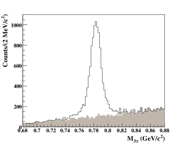
In terms of the mass of the system, , the events were generated according to 3-body phase space weighted by a Voigtian (a convolution of a Breit-Wigner and a Gaussian, see (4.1)) to account for both the natural width of the and detector resolution. For this example, we chose to use MeV/c2 for the detector resolution (see Figure 2). The goal of our analysis is to extract the three measurable elements of the spin density matrix (for the case where neither the beam nor target are polarized) traditionally chosen to be , and . These can be accessed by examining the distribution of the decay products () of the in its rest frame.
For this example, we chose to work in the helicity system which defines the axis as the direction of the in the overall center-of-mass frame, the axis as the normal to the production plane and the axis is simply given by . The decay angles are the polar and azimuthal angles of the normal to the decay plane in the rest frame, i.e. the angles of the vector . The decay angular distribution of the in its rest frame is then given by [2]
| (7) |
which follows directly from the fact that the is a vector particle; it has spin-parity .
We chose to use the following values for this example:
| (8a) | |||
| (8b) | |||
| (8c) |
The resulting generated decay distribution is shown in Figure 1.
For the background, we chose to generate it according to 3-body phase space weighted by a linear function in and
| (9) |
in the decay angles. Figure 2 shows the mass spectrum for all generated events and for just the background. The generated decay angular distributions for all events, along with only the signal and background are shown in Figure 1. There is clearly no way to separate out the signal events through the use of a cut.

4.1 Applying the Procedure
To obtain the -factors, we first need to identify the relevant coordinates, i.e. the kinematic variables in which we need to separate signal from background. The mass will be used as the reference coordinate, . The stated goal of our analysis is to extract the elements. We will do this using (4); thus, only the angles are relevant. Other decay variables, such as the distance from the edge of the Dalitz plot, are not relevant to this analysis — though, they would be in other analyses (see Section 4.4).
Using the notation of Section 2, and the distance between any two points, , is given by
| (10) |
The functional dependence of the signal and background on the reference coordinate, , are
| (11a) | |||
| (11b) |
where GeV/c2, MeV, MeV is the simulated detector resolution, are unknown parameters and
| (12) |
is the convolution of a Gaussian and non-relativistic Breit-Wigner known as a Voigtian ( is the complex error function).
As stated above, the number of nearest neighbor events required depends on the analysis. Specifically, it depends on how many unknown parameters there are, along with the functional forms of and . For this relatively simple case, the value works well. For each simulated event, we then find the closest events (containing both signal and background) and perform an unbinned maximum likelihood fit, using the CERNLIB package MINUIT [3], to determine the estimators . The -factors are then calculated from (3) and the uncertainties are straightforward to calculate using Section 3.
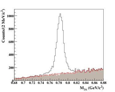
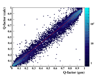
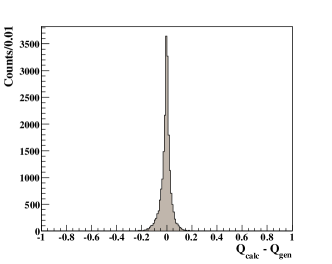
Figure 4 shows the comparison of the extracted and generated background distributions integrated over all decay angles. The agreement is quite good; however, we are looking for more than just global agreement. Figure 3 shows the extracted angular distributions for the signal and background. The agreement with the generated distributions is excellent (see Figure 1) . We can also compare the -factors extracted by the fits to the theoretical distributions from which our data was generated. Figure 5 shows that the extracted values are in very good agreement with the generated values.
We conclude this section by discussing the importance of quality control in the fits. For this example, we performed 20,000 independent fits to extract the -factors. To avoid problems which can arise due to fits not converging or finding local minima, each unbinned maximum likelihood fit was run with three different sets of starting values for the parameters : (1) 100% signal; (2) 100% background; (3) 50% signal, 50% background. In all cases, the fit with the best likelihood was used. The events were then binned and a was obtained. In about 2% of the fits the was very large, a clear indicator that the fit had not found the best estimators . For these events, a binned fit was run to obtain the -factor.
4.2 Examining the Errors
As discussed in Section 3, the covariance matrix obtained from each event’s fit can be used to obtain the uncertainty in , , using (5). The nature of our procedure leads to a high degree of correlation between neighboring event’s -factors. This means that adding the uncertainties in quadrature would definitely underestimate the true error. In Section 3, we argued that a better approach was to assume 100% correlation which provides an overestimate of the true error.
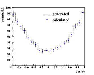
To examine the error bars in our toy example, we chose to project our data into a one-dimensional distribution in . This was done to avoid bin occupancy issues which arise in the two-dimensional case due to limitations in statistics. Figure 6(a) shows the comparison between the generated and calculated distributions. The agreement is excellent. The error bars on the calculated points were obtained using (6). For this study, we ignore the Poisson statistical uncertainty in the yield due to the fact that the number of generated events is known. In a real world analysis, these should be included in the quoted error bars.
We can examine the quality of the error estimation by examining the difference between the generated and calculated yields in each bin, . Figure 6(b) shows the comparison between , obtained assuming 100% correlation and obtained assuming no correlation, i.e. adding the individual uncertainties in quadrature. As expected, the correlated errors provide an overestimate of in every bin, while the uncorrelated errors greatly underestimate in the majority of bins.
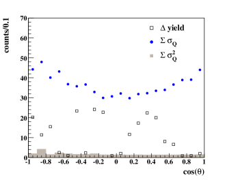
It is not surprising that the errors obtained using (6) are better estimates of the true uncertainty when the bin occupancy is closer to . We could come up with a scheme to scale the size of the error bars according to bin occupancy; however, recall that in this example we fit the background with the functional form to which it was generated. This typically will not be the case for real data. In a real analysis, fitting with different functional forms and examining the extracted signal distributions to estimate systematic effects due to the choice of background is generally required. In this case, one should simply consider that the uncorrelated error bars are overestimates for each choice of background function when estimating the systematic uncertainty in the signal yields.
4.3 Extracting Observables: Event-Based Fitting using -Factors
The goal of our model analysis is to extract the spin density matrix elements. When studying multi-dimensional problems, binning the data is often undesirable due to limitations in statistics. The -factors obtained for each event above can be used in conjunction with the unbinned maximum likelihood method to avoid this difficulty.
If we could cleanly separate out the signal events from the background, then the likelihood function would be defined as
| (13) |
where is the decay angular distribution defined in (4). We could then obtain estimators for the spin density matrix elements by minimizing
| (14) |
In this example, it is not possible to separate the signal and background event samples; however, we can use the -factors to achieve the same effect by rewriting (14) as
| (15) |
where the sum is now over all events (signal and background). Thus, the -factors are used to weight each event’s contribution to the likelihood.
Using the -factors obtained in Section 4.1, minimizing (15) yields
| (16a) | |||
| (16b) | |||
| (16c) |
where the uncertainties are purely statistical (obtained from the fit covariance matrix). Thus, the values extracted for the spin density matrix elements are in excellent agreement with the values used to generate the data given in (8).
4.4 Extending the Example
To extend this example to allow for the case where the data is not binned in production angle, we would simply need to include or in the vector of relevant coordinates, . To perform a full partial wave analysis on the data, we would also need to include any additional kinematic variables which factor into the partial wave amplitudes, e.g. the distance from the edge of the Dalitz plot (typically included in the decay amplitude). We would then construct the likelihood from the partial waves and minimize using the -factors obtained by applying our procedure including the additional coordinates. An example of this can be found in [4].
5 Conclusions
In this paper, we have presented a procedure for separating signals from non-interfering backgrounds by determining, on an event-by-event basis, a quality factor (-factor) that a given event originated from the signal distribution. We have shown that this -factor can be used as an event weight in subsequent analysis procedures to allow more direct access to the true signal distribution. Though this procedure may be computationally expensive, in principle it only needs to be performed once for each event in the data sample.
Acknowledgments
This work was supported by grants from the United States Department of Energy No. DE-FG02-87ER40315 and the National Science Foundation No. 0653316 through the “Physics at the Information Frontier” program.
References
- [1] V. H. Regener, Phys. Rev. 84, 161 (1951).
- [2] K. Schilling, P. Seyboth and G. Wolf, Nucl. Phys. B15, 397 (1970).
- [3] F. James, CERN Program Library D506 (1998).
- [4] M. Williams, Carnegie Mellon University Ph.D. Thesis, (2007).