Backbone and Side-chain Ordering in a Small Protein

Abstract

We investigate the relation between backbone and side-chain ordering in a small protein. For this purpose we have performed multicanonical simulations of the villin headpiece subdomain HP-36, an often used toy model in protein studies. Concepts of circular statistics are introduced to analyze side-chain fluctuations. In contrast to earlier studies on homopolypeptides (Wei et al., J. Phys. Chem. B, 111 (2007) 4244) we do not find collective effects leading to a separate transition. Rather, side-chain ordering is spread over a wide temperature range. Our results indicate a thermal hierarchy of ordering events, with side-chain ordering appearing at temperatures below the helix-coil transition but above the folding transition. We conjecture that this thermal hierarchy reflects an underlying temporal order, and that side-chain ordering facilitates the search for the correct backbone topology.

I Introduction

The process by which a protein folds into its biologically active state cannot be traced in all details solely by experiments. Fortunately, modern simulation techniques have opened another window, often leading to new insight into the dynamics and thermodynamics of folding Scheraga ; Kolinski ; Irbaeck ; Wei ; Skolnick ; Wenzel . Generalized ensemble techniques HO98 such as parallel tempering PT1 ; PT2 ; H97f or multicanonical sampling MU ; MU2 , first introduced to protein science in Ref. HO, , have made it possible to study the folding of small proteins (with up to $\approx 50$ residuesKH05 ) in silico. Of particular interest is whether there are different distinct transitions in the folding process, and what their thermal order and relation is.

An example is the role of side-chain ordering. In recent studies on homopolymers WNH06 ; WNH07a , we found for certain amino acids a de-coupling of backbone and side-chain ordering. The ordering did not depend on the details of the environment, i.e. whether the molecules were in gas phase or solvent, but solely on the particular side groups. It exhibited a transition-like character, marked by an accompanying peak in the specific heat. In the present work we extend this study to proteins, i.e. heteropolymers of amino acids.

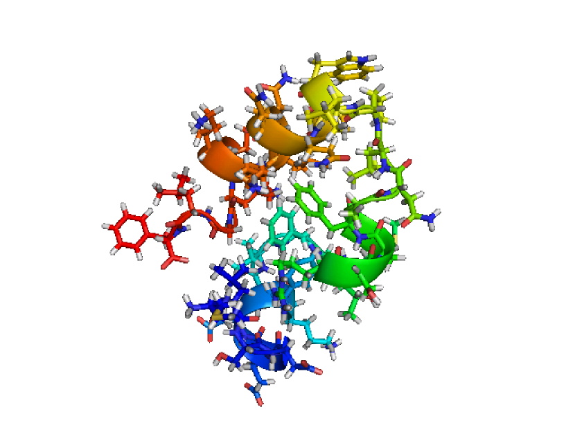
Our test protein is the villin head piece subdomain HP-36 with which we are familiar from earlier work ELP ; HP36 ; TTH06 . This molecule has raised considerable interest in computational biology Freed ; Ripoli as it is one of the smallest proteins (596 atoms) with well-defined secondary and tertiary structure McKnight:96 but at the same time still accessible to simulations Duan:98 . Its structure was resolved by NMR analysis and is shown in Fig. 1 as it is available in the Protein Data Bank PDB (PDB code 1vii). We use multicanonical sampling to study the thermal behavior of the protein in aqueous solvent over a wide range of temperatures from one single simulation. Such an approach is well-suited to overcome the problem of “slowness” of side-chain ordering observed in canonical simulations Shimada ; Kussell .

We observe that side-chain ordering occurs over a wide range in temperatures below the helix-coil transition. Although we do not find the collective effects leading to a separate side-chain ordering transition that were observed for homopolymers  WNH06 ; WNH07a , this result indicates that secondary structure formation is a necessary precursor for side-chain ordering. On the other hand, side-chain ordering occurs at higher temperatures than those at which the protein backbone assumes its native fold. We conjecture that HP-36 folds in a multi-step process, with side-chain ordering facilitating the search for the correct backbone topology.

II Methods

Our simulations utilize the ECEPP/2 force field EC as implemented in the 2005 version of the program package SMMP SMMP ; SMMP05 . Here the interactions between the atoms of the protein are approximated by a sum $E_{ECEPP/2}$ consisting of electrostatic energy $E_{C}$, a Lennard-Jones term $E_{LJ}$, hydrogen-bonding term $E_{HB}$ and a torsion energy $E_{Tor}$:

$$E_{\text{ECEPP/2}} = E_{C}+E_{LJ}+E_{HB}+E_{Tor}$$ (1)

$$= \sum_{(i,j)}\frac{332q_{i}q_{j}}{\epsilon r_{ij}}$$

$$+\sum_{(i,j)}\left(\frac{A_{ij}}{r_{ij}^{12}}-\frac{B_{ij}}{r_{ij}^{6}}\right)$$

$$+\sum_{(i,j)}\left(\frac{C_{ij}}{r_{ij}^{12}}-\frac{D_{ij}}{r_{ij}^{10}}\right)$$

$$+\sum_{l}U_{l}(1\pm\cos(n_{l}\xi_{l}))\;,$$

where $r_{ij}$ is the distance between the atoms $i$ and $j$, $\xi_{l}$ is the $l$-th torsion angle, and energies are measured in kcal/mol. The protein-solvent interactions are approximated by a solvent accessible surface term

$$E_{solv}=\sum_{i}\sigma_{i}A_{i}\;.$$ (2)

The sum is over the solvent accessible areas $A_{i}$ of all atoms $i$ weighted by solvation parameters $\sigma_{i}$ as determined in Ref. OONS, , a common choice when the ECEPP/2 force field is utilized. Our previous experiences PTH ; TTH06 have shown that $E_{solv}$ reproduces the effects of protein-water interaction qualitatively correct. However, the temperature scale is often distorted, leading, for instance, to transitions at temperatures where water would be vaporized in nature. This problem can be remedied, however, by renormalization of the temperature scale upon comparison with experiments.

The above defined energy function leads to a landscape that is characterized by a multitude of minima separated by high barriers. As the probability to cross an energy barrier of height $\Delta E$ is given by $\exp(-\Delta E/k_{B}T)$, $k_{B}$ being the Boltzmann constant, it follows that extremely long runs are necessary to obtain sufficient statistics in regular canonical simulations at low temperatures. Hence, in order to enhance sampling we rely on the multicanonical approach MU ; MU2 as described in Ref. HO, . Here, configurations are weighted with a non-canonical term $w_{MU}(E)$ usually determined iteratively to optimize certain properties of the simulation. Thermodynamic averages of an observable $<O>$ at temperature $T$ are obtained by re-weighting FS :

$$<O>(T)=\frac{\int dx\;O(x)e^{-E(x)/k_{B}T}/w_{MU}[E(x)]}{\int dx\;e^{-E(x)/k_{B}T}/w_{MU}[E(x)]}$$ (3)

where $x$ counts the configurations of the system.

Most often the multicanonical weight is determined such that the probability distribution obeys

$$P_{MU}(E)\propto n(E)w_{MU}(E)\approx const~{},$$ (4)

where $n(E)$ is the spectral density of the system. However, in our implementation we do not require a constant histogram but that the number of round-trips $n_{rt}$ between two pre-set low and high energy values $E_{low}$ and $E_{high}$ is maximal. $E_{high}$ is a an energy value typical for an disordered high temperature state (in our example $E_{high}$ = -133.5 kcal/mol) while $E_{low}=-357$ Kcal/mol was chosen to correspond to typical low-energy states as determined by us in preliminary studies. Obviously, the number of round-trips $n_{rt}$ between the lowest and highest temperature, $E_{low}$ and $E_{high}$, respectively, is a lower bound for the statistically independent visits at the low energy states, and therefore a good measure for the efficiency of the simulation. For this reason, it is desirable to maximize the number of round trips by optimizing $w_{MU}(E)$. This can be achieved in a systematic way by the feedback algorithm described in Refs. THT, ; NH, . The resulting weights are given as supplemental material.

A simulation of five million Monte Carlo sweeps (each consisting of 217 Metropolis steps that try to update all 217 dihedral angles of the molecule once) leads to 35 tunneling events, i.e. at least 35 independent configurations with energies smaller than $-357$ kcal/mol. Every ten sweeps, we measure the energy $E$ with its respective contributions from Eq. (1) and from the protein-solvent interaction energy $E_{solv}$. Other quantities measured are the radius of gyration $R_{gy}$ as a measure of the geometrical size, and the number of helical residues $n_{H}$, i.e. residues where the pair of dihedral angles $(\phi,\psi)$ takes values in the range ($-70^{\circ}\pm 30^{\circ}$, $-37^{\circ}\pm 30^{\circ}$) Okamoto1995 . Also we monitor the $RMSD$ (root mean square deviation) of various subsets of heavy atoms (backbone, sidechain, all) from the PDB structure.

Finally, all the 217 dihedral angles are recorded for later analysis of their fluctuations and correlations. As the statistical analysis of dihedral angles has subtle pitfalls, we present and justify our approach in the Appendix.

III Results and Discussions

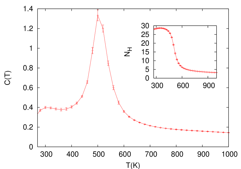
Multicanonical simulations allow determining thermodynamic quantities over a wide range of temperatures. The thermal evolution of the specific heat, for example,

$$C(T)=\frac{d}{dT}E=k_{B}\beta^{2}\left(<E^{2}>-<E>^{2}\right)$$ (5)

provides information about the temperatures where the protein changes its state. In earlier investigations WNH06 ; WNH07a of homopolymers we observed two separate peaks in the specific heat for particular amino acids, characterizing two well-defined transitions. One peak was associated with a helix-coil transition, i.e. the ordering of the protein backbone. The second peak, at a much lower temperature, could be related to an ordering of side chains. These results indicated a two-step folding process upon lowering the temperature, starting with backbone ordering followed by side-chain ordering. How does the situation look like for a heteropolymer such as HP-36?

The specific heat curve in Fig. 2 has only one marked peak at $T=505\pm 8$ K; but it also exhibits a shoulder around T=$300$K. As for the homopolymers, the peak in the specific heat can be related to a helix-coil transition. This interpretation is supported by the inset where we display the average number $<n_{H}>$ of residues that are part of an $\alpha$-helix as a function of temperature. The steep increase in this quantity at $T=505$K is clearly correlated with the peak in the specific heat.

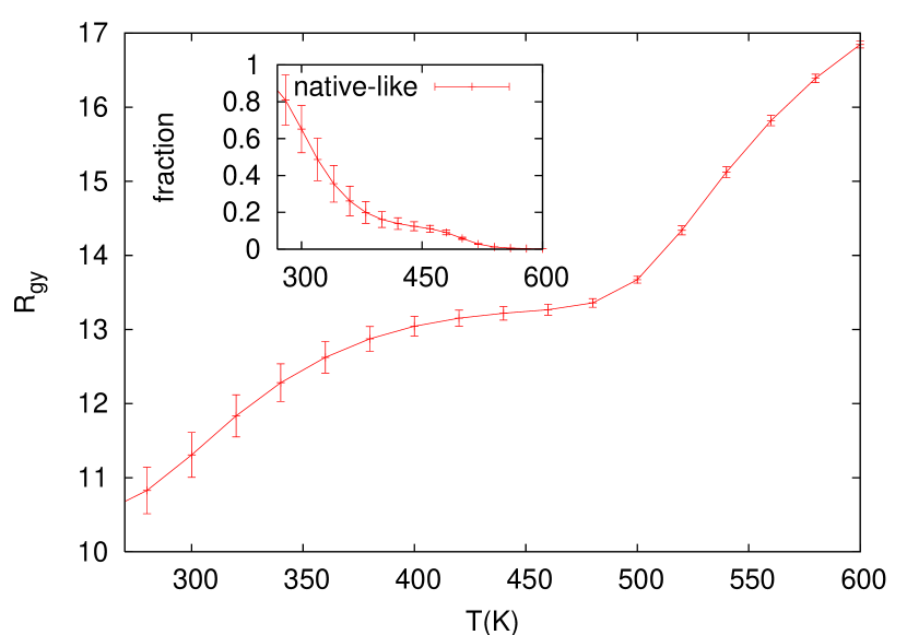
However, for HP-36 backbone ordering is more than just the formation of secondary structure. The average radius of gyration $<R_{gy}>$, a measure for the compactness of a protein configuration, as a function of temperature, is displayed in Fig. 3. It indicates that backbone ordering occurs in more than one step. Below $T=505$ K, most protein configurations have a high helix propensity. Lowering the temperature further, compact structures become finally more frequent than extended configurations with equal or even higher helicity. This two-step process in the backbone ordering can also be seen in the inset which displays the fraction of configurations with a $RMSD$ smaller than 6 Å, i.e. those that should fall within the free energy basin of the native structure ScheragaOrSo . Final compactification and transition to nativeness are therefore concomitant processes. We believe that the shoulder in the specific heat is correlated with that final backbone ordering since it occurs close to the steepest parts of the decrease of $<R_{gy}>$ and the increase of nativeness.

Hence, our results so far indicate a two-step process, but one that involves only the backbone. The first step, correlated with a critical temperature $T=505$ K involves the formation of helical segments. In a second step, these arrange themselves to compact and native-like structures. The energy gain here is much smaller, and therefore this second ordering step is observed at lower temperatures only.

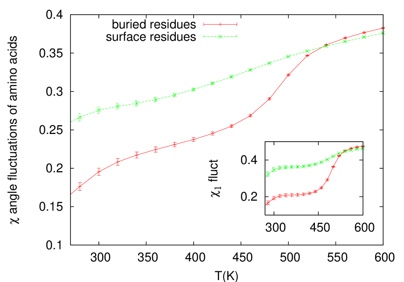
How does side-chain ordering fit into this picture? The behavior of the specific heat does not give any indications of a separate transition related to side-chain ordering. Such a transition could still exist — albeit not associated with large energy fluctuations. A quantity that describes side-chain ordering in a very general way is the average of the fluctuations of dihedral angles. We have calculated this quantity as described in the appendix for buried side chains and compare it with fluctuations of angles belonging to side chains at the surface of the molecule. Both quantities are displayed in Fig. 4 for all angles of a side chain, and in the inset solely for the $\chi_{1}$ angle. For the buried residues one observes a single step ordering of the side chains. Immediately below the helix-coil transition the fluctuations decrease, indicating that here the formation of helical segments leads already to some ordering of side chains. In the temperature range $300-500$ K the fluctuations decrease further, albeit less dramatic. This range corresponds to the shoulder in the specific heat and marks compactification and the formation of the tertiary backbone structure. Residues at the surface exhibit a much smaller decrease of fluctuations associated with the formation of helical segments.

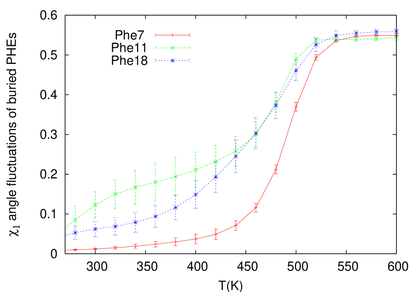
At higher temperatures, side-chain ordering is restricted to residues in the interior of a protein. This is reasonable as here the side chain positions are more constraint by the geometry of the molecule. For this reason, we have focused our further analysis on side chain angles of residues in the interior of the molecule. Fig. 5 shows the fluctuations of the $\chi_{1}$ angle for the residues Phe₇, Phe₁₁ and Phe₁₈. Fluctuations of these angles decrease strongly over a small range of temperatures below the formation of the helical segments. We note that Phe₇ exhibits ordering at a somewhat higher temperature than Phe₁₁ and Phe₁₈.

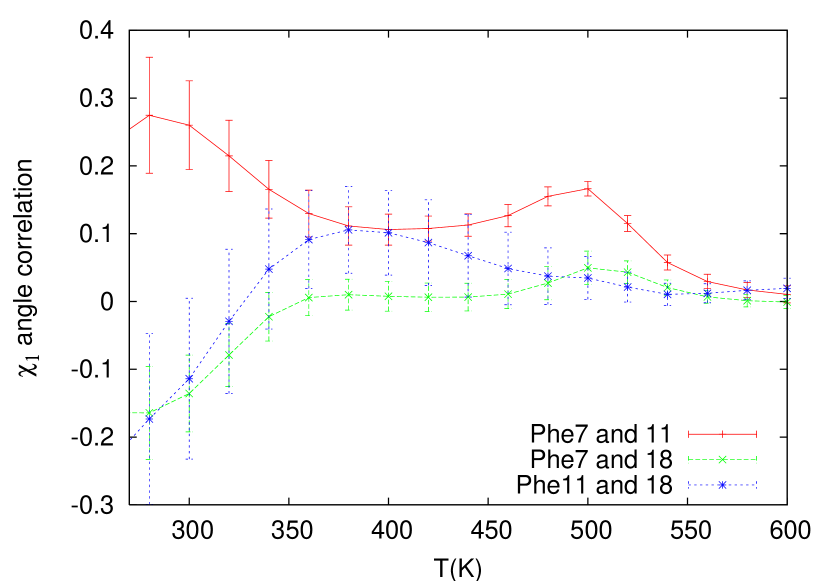
The decrease in fluctuations is only loosely related to an increase in correlations between the $\chi_{1}$ angles of these three residues, see Fig. 6, where the data were determined as described in the appendix. Phe₇ exhibits correlated fluctuations with Phe₁₁ already close to the helix coil transition. They persist and increase finally in the low temperature phase. Phe₇ and Phe₁₈ exhibit (anti-)correlations only below $350$ K. The most dramatic change occurs with Phe₁₁ and Phe₁₈: Their correlations start to occur around $450$ K, i.e. just when those angles are ordering; however, upon lowering the temperature the correlations switch to anti-correlations and increase in magnitude.

Note, that all correlated fluctuations of these side chains exhibit their steepest change below $350$ K, where Fig. 3 and its inset indicate the folding transition into the native backbone topology. On the other hand, this is the regime where angle fluctuations have subsided already. Hence, for HP-36 the correct ordering of the side chains seem to predate tertiary structure formation. These results also indicate that the final arrangement of the side chains occurs collectively.

The above results indicate the following sequence of events in the folding of villin headpiece subdomain HP-36 upon lowering the temperature. The first stage is the formation of helical segments, connected with a large gain in potential energy. Below this helix-coil transition is a large intermediate temperature range where various helical configurations other than the native one dominate for entropic reasons. This temperature range is also characterized by an increased side-chain ordering that is more pronounced for side chains of residues in the interior that arrange themselves in coordinated way. The heterogeneity of the sequence seems to destroy the phase transition-like character of side-chain ordering that was observed by us for some homopolymers. Instead, the ordering is more gradual. Only at temperatures below side-chain ordering, and connected with a much smaller gain in energy than at the helix-coil transition, do the helical segments arrange themselves in native-like structures.

Our results show a particular thermal order of the folding processes. It is natural to assume that this thermal order reflects a related temporal order of folding events. Hence, we conjecture that HP-36 folds in multi-step process where side chain and backbone ordering are interconnected. The initial step is the formation of helical segments. In a second step the protein collapses into more compact structures before it assumes its native state. This sequence of events is consistent with various computational Lei ; Pande ; Mori and experimental Kubelka2003 studies that also identify the formation of helical segments as the time limiting factor in the folding of HP-36. New is our observation that the search for the correct structure seems to be facilitated by the ordering of side chains subsequent to secondary structure formation. This scenario is also consistent with recent mutagenesis experiments (relying on nanosecond laser T-jump measurements) that emphasize the importance of buried side chains for the rather short folding times of the villin headpiece Kubelka2003 ; Kubelka2006 .

IV Summary and Outlook

Choosing a well-studied small protein, the villin headpiece subdomain HP-36, we have presented methods that allow us to simulated and analyze ordering processes taking place on the level of the side chain dihedral angles as well as at the level of the backbone structures. Our results indicate a thermal hierarchy of ordering events with side-chain ordering appearing at temperatures below the helix-coil transition but above the folding transition. We believe that the observed thermal hierarchy of folding reflects an underlying temporal sequence of these ordering processes in actual protein folding dynamics. We conjecture that side-chain ordering facilitates the search for the correct backbone topology. Further studies along these lines on different proteins will elucidate how general such a scenario is.

Acknowledgments Support by a research grant (CHE-0313618) of the National Science Foundation (USA) is acknowledged.

Appendix A Statistical Analysis of Dihedral Angles

Correct statistical analysis of dihedral angles is somewhat subtle because of their periodicity modulo $2\pi$. This property excludes the use of regular statistical measures like the mean angle, $\left<\alpha\right>$, or its variance, $\left<(\alpha-\left<\alpha\right>)^{2}\right>$. The reason is that the numerical values of those quantities depend on the reference frame chosen, e.g. $\left[-\pi,\pi\right]$ or $\left[0,2\pi\right]$ or any other interval of length $2\pi$. Moreover, choosing an inappropriate reference frame can lead, e.g. to the spurious appearance of a bimodal distributions from an underlying unimodal one.

On the other hand, there exist the well-established mathematical fields of circular or directional statistics Fisher1995 ; Mardia1999 ; Topics2001 that deal with such problems. However, we believe that some the quantities and equations used there introduce unnecessary complications and do not fully reflect the underlying physical concepts. So, here we will borrow some ideas from that field, but we will not fully follow that approach.

The important fundamental idea introduced in circular and directional statistics is that an angle $\alpha$ can be viewed as a two-dimensional vector of unit length

$${\bf a}={\cos(\alpha)\choose\sin(\alpha)}\quad,$$ (6)

a concept that bears some similarity to, e.g., a spin in an XY-model XYmodel treated in statistical physics. Consequently, we are interested in the mean direction ${\overline{{\bf a}}}$, also considered to be a unit vector. It can be determined from the averaged vector

$$\left<{\bf a}\right>={\left<\cos(\alpha)\right>\choose\left<\sin(\alpha)\right>}\quad.$$ (7)

which is usually smaller than a unit vector,

$$R^{2}(\alpha)=\left<\cos(\alpha)\right>^{2}+\left<\sin(\alpha)\right>^{2}<1\quad,$$ (8)

by

$${\overline{{\bf a}}}=\frac{1}{R(\alpha)}\left<{\bf a}\right>$$ (9)

From this mean direction vector a corresponding mean angle ${\overline{\alpha}}$ could be determined in an appropriate frame,

$${\overline{{\bf a}}}\equiv{\cos({\overline{\alpha}})\choose\sin({\overline{\alpha}})}\quad.$$ (10)

Notice that - as we will see below - most often it is not necessary to determine that angle. Rather, it is sufficient to work with either the mean vector $\left<{\bf a}\right>$, Eq. (7), or the mean direction vector ${\overline{{\bf a}}}$ , Eq. (9).

In this contribution we concentrate mostly on $fluctuations$ and $correlations$ between dihedral angles. Correlation analysis, in particular, is a somewhat complex field in the directional statistics literature, sometimes motivated and dominated by the fact that the underlying data are temporal and the goal is the detection of circadian rhythms Fisher1995 ; Mardia1999 . Moreover, the quantities employed for describing fluctuations do not always match up with those employed for describing correlations. Below we sketch the problems and justify our approach.

The simplest measure for fluctuations is based on the length of the average vector, Eq. (8). The circular variance is given simply by

$$V\left(\alpha\right)=1-R\left(\alpha\right)\quad.$$ (11)

$V=0$ corresponds to vanishing fluctuations, while $V=1$ describes the case of an equidistribution of angles over the full range, i.e. maximal fluctuations. Interestingly, the circular variance can be derived, too, by considering the deviation vectors from the mean direction, i.e.

$$V\left(\alpha\right) = \frac{1}{2}\left<\left|{\bf a}-{\overline{{\bf a}}}\right|^{2}\right>$$ (12)

$$= \frac{1}{2}\left(\left<{\bf a}^{2}\right>-2\left<{\bf a}\right>\cdot{\overline{{\bf a}}}+{\overline{{\bf a}}}^{2}\right)$$

$$= 1-R(\alpha)\quad.$$

Ideally, in order to systematically analyze correlations and fluctuations together, a covariance function $C\left(\alpha_{i},\alpha_{j}\right)$ is necessary that generalizes the fluctuation measure employed. Combining the chosen covariance and fluctuation functions, the correlation matrix is finally given by

$$\rho\left(\alpha_{i},\alpha_{j}\right)=\frac{C\left(\alpha_{i},\alpha_{j}\right)}{\sqrt{V(\alpha_{i})V(\alpha_{j})}}\quad.$$ (13)

$\rho=0$ denotes vanishing correlations, either since there are no fluctuations at all, or because the fluctuations are uncorrelated. $\rho\to\pm 1$ corresponds to full correlation or anti-correlation of the fluctuations, respectively.

Unfortunately, a straightforward extension from Eqs. (11) and (12), e.g. defining the covariance function as the scalar product of the respective deviation vectors from the mean direction, $C\left(\alpha_{i},\alpha_{j}\right)\propto\left<\left({\bf a}_{i}-{\overline{{\bf a}_{i}}}\right)\cdot\left({\bf a}_{j}-{\overline{{\bf a}_{j}}}\right)\right>$, is not possible. This quantity does not vanish if the angles are statistically independent, as it should for a proper covariance. Instead, replacing the deviations from the mean direction by the deviations from the mean vector does result in a seemingly proper covariance function,

$$C_{\rm diff}\left(\alpha_{i},\alpha_{j}\right)=\left<\left({\bf a}_{i}-\left<{\bf a}_{i}\right>\right)\cdot\left({\bf a}_{j}-\left<{\bf a}_{j}\right>\right)\right>\quad.$$ (14)

The related variance function differs from Eq. (11) though,

$$V_{\rm diff}\left(\alpha\right) = \left<\left|{\bf a}-\left<{\bf a}\right>\right|^{2}\right>=\left<{\bf a}^{2}\right>-\left<{\bf a}\right>^{2}$$ (15)

$$= 1-\left[\left<\cos(\alpha)\right>^{2}+\left<\sin(\alpha)\right>^{2}\right]$$

$$= 1-R^{2}(\alpha)\quad.$$

Both forms, $V\left(\alpha\right)$ and $V_{\rm diff}\left(\alpha\right)$, are related by a monotonic — albeit nonlinear — mapping and describe fluctuations in a qualitatively similar way. The only quantitative difference is that Eq. (15) better resolves the small fluctuation regime while Eq. (11) does that with the regime of large fluctuations.

While we do not consider the changed variance to be a problem, there is one with Eq. (14). Although $C_{\rm diff}\left(\alpha_{i},\alpha_{j}\right)$ exhibits the correct behavior in the limit of statistical independence of the angles, we have observed that problems arise in the regime of larger correlations. This is due to the fact that $\left|\left<{\bf a}_{i}\right>\right|\neq\left|\left<{\bf a}_{j}\right>\right|$ usually holds, which leads to an imbalance in the treatment of the respective deviation vectors.

The authors of Ref. Topics2001, suggest to describe correlations between angles by the covariance function

$$C_{\sin}\left(\alpha_{i},\alpha_{j}\right)=\left<\sin(\alpha_{i}-{\overline{\alpha_{i}}})\sin(\alpha_{j}-{\overline{\alpha_{j}}})\right>\quad,$$ (16)

This function also exhibits the correct behavior for independently distributed angles, and - again - the related variance function differs from Eq. (11),

$$V_{\sin}\left(\alpha\right)=\left<\sin^{2}(\alpha-{\overline{\alpha}})\right>\quad.$$ (17)

Notice that this measure of fluctuations necessarily includes higher order moments of the angular trigonometric functions than those Eqs. (11) and (15) use. Consequently, there does not exist a simple analytic mapping to the circular variance, and - particularly for large fluctuations - a non-monotonic relationship is possible footnoteNonMonotonic .

We note that, as mentioned above, it is actually not necessary to determine the average angle ${\overline{\alpha}}$ explicitly for evaluating Eq. (16). Rather, this equation also has a vector representation, albeit by using the cross product of vectors in addition to the scalar product. Extending ${\bf a}$ to a 3d vector via

$${\hat{{\bf a}}}=\left(\begin{array}[]{c}\cos(\alpha)\\ \sin(\alpha)\\ 0\\ \end{array}\right)\quad,$$ (18)

and using trigonometric identities, it can be easily seen that the the sine of the angle difference is given by the $z$-component of the cross product $(-{\hat{{\bf a}}}\times{\overline{\hat{{\bf a}}}})$. Consequently, the covariance (16) can be represented as

$$C_{\sin}\left(\alpha_{i},\alpha_{j}\right)=\left<\left({\hat{{\bf a}}_{i}}\times{\overline{\hat{{\bf a}}_{i}}}\right)\cdot\left({\hat{{\bf a}}_{j}}\times{\overline{\hat{{\bf a}}_{j}}}\right)\right>\quad.$$ (19)

Analogously, the corresponding fluctuations are represented via

$$V_{\sin}(\alpha)=\left<\left|{\hat{{\bf a}}_{i}}\times{\overline{\hat{{\bf a}}_{i}}}\right|^{2}\right>\quad.$$ (20)

As outlined above, we would have preferred to systematically analyze fluctuations and correlations together, either using Eqs. (15) and (14), or Eqs. (17) and (16). However, the problems with the covariance Eq. (14) — imbalance in the large correlations regime — and the variance Eq. (17) — non-monotonicity in the large fluctuations regime — do not allow this.

Rather, we decided to employ a hybrid approach: When dealing with fluctuations we always rely on the circular variance, Eqs. (11) since it is the simplest reliable approach. When dealing with correlations, we use the covariance $C_{\sin}\left(\alpha_{i},\alpha_{j}\right)$, Eq.(16). Necessarily, we have to employ the problematic variance $V_{sin}(\alpha)$, Eq.(17), as normalization in determining the correlation function $\rho\left(\alpha_{i},\alpha_{j}\right)$, Eq. (13). Since in our case correlations arise only in the regime where fluctuations are small, we feel that is an acceptable approach. It also outweighs the problems that arise from using Eq. (14).

We emphasize in closing that — to our knowledge — no satisfying approach exists yet to treat strong dihedral angle correlations in the large fluctuations regime.

Figure captions:

Fig. 1: Structure of HP-36 (picture was obtained by VMD  vmd ).

Fig. 2: Specific heat as a function of temperature. The inset displays the helicity as a function of temperature.

Fig. 3: Radius of gyration as a function of temperature. The inset shows the fraction of configurations with a backbone RMSD from the PDB structure less than 6 Å.

Fig. 4: Averaged fluctuations, Eq. (11), of side chain angles from buried and surface side groups, respectively; the inset shows average of only the $\chi_{1}$ angle fluctuations. Note the errorbars denote the average of the errors in the fluctuations of each individual $\chi$ angle.

Fig. 5: Averaged fluctuations, Eq. (11), of $\chi_{1}$ for Phe7, Phe11, and Phe18.

Fig. 6: Correlations, Eq. (13), based on Eqs. (16) and (17), of $\chi_{1}$ fluctuations between Phe7 and Phe11, Phe7 and Phe18, and Phe11 and Phe18, respectively; see also the discussion in the appendix.

Figure 1:

Figure 2:

Figure 3:

Figure 4:

Figure 5:

Figure 6:

References

- (1) A. Ghosh, R. Elber and H. Scheraga, Proc. Natl. Acad. Sci. (USA) 99, 10394 (2002).
- (2) S. Kmiecik and A. Kolinski, Proc. Natl. Acad. Sci. 104 12330 (2007).
- (3) G. Favrin, A. Irbäck, and S. Wallin, Proteins: Struct., Funct., Genet. 47, 99 (2002).
- (4) H. Li, M. Fajer and W. Yang, J. Chem. Phys. 126 24106 (2007).
- (5) A. Jagielska and J. Skolnick, Journal of Computational Chemistry 28(10) 1648 (2007).
- (6) T. Herges and W. Wenzel, Biophys. J. 87, 3100 (2004).
- (7) U.H.E. Hansmann and Y. Okamoto, in D. Stauffer (ed.) Annual Reviews in Computational Physics VI (Singapore, World Scientific; 1999) p.129-157.
- (8) C.J. Geyer and A. Thompson, J. Am. Stat. Ass. 90, 909 (1995).
- (9) K. Hukushima and K. Nemoto, J. Phys. Soc. (Jpn.) 65, 1604, (1996).
- (10) U.H.E. Hansmann, Chem. Phys. Lett. 281, 140, (1997).
- (11) B.A. Berg and T. Neuhaus, Phys. Lett. B 267, 249, (1991).
- (12) B.A. Berg and T. Celik, Phys. Rev. Lett. 69. 2292 (1992).
- (13) U.H.E. Hansmann and Y. Okamoto, J. Comp. Chem. 14, 1333, (1993).
- (14) W. Kwak and U.H.E. Hansmann, Phys. Rev. Lett. 95, 138102, (2005).
- (15) Y. Wei, W. Nadler, and U.H.E. Hansmann, J. Chem. Phys. 125 , 164902, (2006).
- (16) Y. Wei, W. Nadler, and U.H.E. Hansmann, J. Phys. Chem. B, 111, 4244 (2007).
- (17) U.H.E. Hansmann and L. Wille, Phys. Rev. Let., 88, 068105 (2002).
- (18) C.Y. Lin, C.K. Hu and U.H.E. Hansmann, Proteins:Structure, Function and Genetics, 52, 436 (2003).
- (19) S. Trebst, M. Troyer and U.H.E. Hansmann, J. Chem. Phys., 124, 174903 (2006).
- (20) M.Y. Shen and K.F. Freed, Proteins 49 439 (2002).
- (21) D.R. Ripoli , J.A. Vila and H.A. Scheraga J. Mol. Biol. 339 915 (2004).
- (22) McKnight, C.J., Matsudaira, P.T., Kim, P.S., Nat. Struct. Biol. v4 pp. 180-184, (1997)
- (23) Y. Duan and P.A. Kollman, Science 282, 740 (1998).
- (24) http://www.rcsb.org/pdb/explore/explore.do?structureId=1VII
- (25) http://www.ks.uiuc.edu/Research/vmd/
- (26) J Shimada, E. Kussell, and E. I. Shakhnovich, J. Mol. Biol. 308, 79 (2001).
- (27) E. Kussell and E. I. Shakhnovich, Phys. Rev. Lett. 89, 168101 (2002).
- (28) M.J. Sippl, G. Némethy, and H.A. Scheraga, J. Phys. Chem. 1984, 88, 6231-6233, and references therein.
- (29) F. Eisenmenger, U.H.E. Hansmann, Sh. Hayryan, C.-K. Hu, Comp. Phys. Comm. 138, 192 (2001).
- (30) F. Eisenmenger, U.H.E. Hansmann, Sh. Hayryan, C.-K. Hu, Comp. Phys. Comm. 174, 422(2006).
- (31) T. Ooi, M. Obatake, G. Nemethy, and H.A. Scheraga, Proc. Natl. Acad. Sci. USA 8, 3086 (1987).
- (32) U.H.E. Hansmann , J. Chem. Phys. 120, 417 (2004).
- (33) A.M. Ferrenberg and R.H. Swendsen, Phys. Rev. Lett. 1988, 61, 2635-2638; Phys. Rev. Lett. 1989, 63, 1658(E) and references given in the erratum.
- (34) S. Trebst, D.A. Huse, and M. Troyer, Phys. Rev. E 70, 046701 (2004).
- (35) W. Nadler and U.H.E. Hansmann, Phys. Rev. E 75, 036702 (2007)
- (36) Y. Okamoto and U.H.E. Hansmann, J. Phys. Chem. 99, 11276 (1995).
- (37) The threshold of 6 Å to characterize native-like structures follows remarks by H.A. Scheraga at CBSB06, Jülich (Germany) June 6-9, 2006.
- (38) H.lei, C. Wei, H. Liu and Y. Duan, Proc. Natl. Acad. Sci. (USA) 104 4930 (2007)
- (39) G.M.S. De Mori, G. Colombo and M. Micheletti, Proteins: Struct. Func. Bioinf. 58 459 (2005)
- (40) G. Jayachandran, V. Vishal and V.S. Pande, J. Chem. Phys. 124 164902 (2006)
- (41) J. Kubelka, W.A. Eaton and J. Hofrichter, J. Mol. Biol. 329 625 (2003).
- (42) J. Kubelka, T.K. Chiu, D.R. Davies, W.A. Eaton and J. Hofrichter, J. Mol. Biol. 359 546 (2006).
- (43) N.I. Fisher, Statistical Analysis of Circular Data (Cambridge, Cambridge University Press, 21995).
- (44) K.V. Mardia and P.E. Jupp, Directional Statistics (New York, Wiley, 1999).
- (45) S. Rao Jammalamadaka and A. SenGupta, Topics in Circular Statistics (Singapore, World Scientific, 2001).
- (46) L.P. Kadanoff, Statistical Physics : Statics, Dynamics and Renormalization (Singapore, World Scientific , 2000 ).
- (47) For example, for angles distributed equally in the interval , the resulting variance is . Clearly, larger fluctuations give rise to oscillations in . Consequently, only the range describes fluctuations somewhat reliably, the latter value holding for an equidistribution of angles.