CARTE: pretraining and transfer for tabular learning

Abstract

Pretrained deep-learning models are the go-to solution for images or text. However, for tabular data the standard is still to train tree-based models. Pre-training or transfer is a huge challenge as in general tables have columns about different quantities and naming conventions that vary vastly across sources. Data integration tackles correspondences across multiple sources: schema matching for columns, and entity matching for entries. We propose a neural architecture that does not need such matches. As a result, we can pretrain it on background data that has not been matched. The architecture –CARTE for Context Aware Representation of Table Entries– uses a graph representation of tabular (or relational) data to process tables with different columns, string embeddings of entries and columns names to model an open vocabulary, and a graph-attentional network to contextualize entries with column names and neighboring entries. An extensive benchmark shows that CARTE facilitates learning, outperforming a solid set of baselines including the best tree-based models. CARTE also enables joint learning across tables with unmatched columns, enhancing a small table with bigger ones. CARTE opens the door to large pretrained models embarking information for tabular data.

1 Introduction

The wide availability of pre-trained models has greatly facilitated machine learning for various data modalities, for example with images (Simonyan & Zisserman, 2015) or texts (Devlin et al., 2019). These models can be downloaded from model hubs, embarking a lot of implicit information and transformations that unleashes the power of deep learning even on small datasets. This paradigm has led to the revolution of foundation models (Bommasani et al., 2021) such as large language models (Touvron et al., 2023). But this revolution has not happened for tabular data despite its huge importance for enterprise and institutional data. One roadblock is that integrating data from tables in the wild is often difficult, sometimes impossible. Different tables might not have any related data and when they do, data integration is a whole field of database research (Doan et al., 2012). One might need to solve correspondence across columns –schema matching– or across data sources with different naming conventions for entries –entity matching.

For lack of matching schemas and entities, pretraining across tables in the wild has so far not been possible. Lack of pretraining reduces the benefit of deep architectures, and applications often rely on tree-based methods (Grinsztajn et al., 2022). Here we introduce a learning architecture that enables bypassing schema and string matching by using a graph representation of tables as well as embeddings for all symbols (column names, table entries). The architecture, dubbed CARTE (Context-Aware Representation of Table Entries), is pretrained on a large knowledge base, to capture information on a vast amount of entities and relations. It can then be fine-tuned on a given downstream task, helping learning even in few shot settings. It can also be used for joint learning across multiple tables, enriching a target table with weakly related sources.

In section 2 we present related work; in section 3 we describe the CARTE architecture and training procedures; and in section 4 we ran an extensive empirical study across many tabular datasets, benchmarking the settings of a single downstream table as well as multiple related ones.

2 Related Works

Tabular deep learning

Tables are central to many applications. As a result, numerous deep learning methods tailored for this modality have been proposed (Abutbul et al., 2020; Arik & Pfister, 2020; Popov et al., 2019; Gorishniy et al., 2023b; Somepalli et al., 2021). However, their superiority over tree-based methods has been challenged (Grinsztajn et al., 2022; Shwartz-Ziv & Armon, 2021) especially when accounting for speed or robustness (Gardner et al., 2022). While this debate is ongoing, with McElfresh et al. (2023) claiming that neural networks perform well on certain types of tables, and promising architectures recently published (Gorishniy et al., 2023a; Chen et al., 2023), the difficulty of making significant improvements over tree-based methods suggests that deep learning must bring something more to the fight, such as background knowledge.

Transfer learning for tabular data

Most transfer learning has studied the “conventional” settings: transferring across datasets with the same features i.e. columns. Somepalli et al. (2021) demonstrates pre-training on a larger unlabeled version of the table to improve prediction, while Levin et al. (2023) argues that transfer learning bridges the gap between deep learning and tree-based models in settings where there are few data points but large related datasets, such as in their medical setting. In addition, they consider new or missing features in the downstream table, though this requires exact matching between most features.

XTab (Zhu et al., 2023) can work on tables with different columns using data-specific featurizers that map instances to the same dimension followed by federated learning on the common block. However, they did not outperform tree-based models (CatBoost, Dorogush et al., 2018). Transtab (Wang & Sun, 2022) also vectorizes each row of tables into an embedding space to learn across tables, demonstrating data accumulation across multiple clinical trials to outperform baselines including XGBoost (Chen & Guestrin, 2016). These approach benefit from a pool of tables in the subtopic, but it is not clear if they can be adapted to build pretrained models for a wide set of applications.

Pretrained models for tabular data

TabPFN (Hollmann et al., 2023) has made an interesting step in the direction of pre-trained models for tabular learning: it uses a transformer model pre-trained on large amounts of synthetic data to capture the inductive biases of tabular data, leading to very strong performance on small datasets, though it has no dedicated handling for categorical columns, a challenge of tables where trees historically shine.

Discrete entries

One challenge of tables –much more tackled by the database literature than the machine learning one– is that many of the entries are discrete, represented as strings. Cerda & Varoquaux (2022) created string-based representations that facilitate learning. The TableVectorizer in Skrub (2024) uses these heuristically to turn columns of different types into numerical matrices well suited for learning. Cvetkov-Iliev et al. (2023) contributed KEN, another approach to embed table entities, closer to our goals of pretraining. They create embeddings of all entities in a knowledge graph, capturing the information in a source such as Wikipedia. These embeddings facilitate learning, but the challenge is that each entry of a column must be linked to a Wikipedia entry.

Data integration

Traditional statistical models need data assembled in a single consistent table, which is tackled by the data integration literature (Doan et al., 2012). Finding correspondences between columns across data sources is known as schema matching. Entity matching is a challenge common to data integration and natural language processing (NLP), where a string must be linked to an entity: a unique concept. For instance “Davinci” may denote the historical figure “Leonardo da Vinci”, but also OpenAI “Text-Davinci-003” GPT3 API. Entity matching must be robust to string variations, but most importantly it must account for the context in which an entity appears to disambiguate potential matches. In NLP, pretrained attention-based models, such as BERT (Devlin et al., 2019), have been crucial to capture the corresponding context.

These pretrained language models have actually been shown on tables to be useful to automate data normalization and integration tasks with few manually-supplied examples per table (Narayan et al., 2022). Deep learning, and more recently attention-based models, is progressing on tasks to structure databases, e.g. column typing, entity linking (Hulsebos et al., 2019; Deng et al., 2020).

We are interested in a different problem, capturing only implicit data structure and integration to enhance downstream machine learning task without any manual operation such as finding related sources. The problem is timely: researchers sharing this vision are assembling large corpora of tables (Hulsebos et al., 2023; Eggert et al., 2023). Yet, the small scale of most tables available and the variability between tabular datasets has so far made this vision elusive.

3 The CARTE model to learn across tables

The ability of CARTE to learn across tables stems from the combination of two elements: a novel representation of table entities with graphs and a deep neural network architecture that captures the context that reside within a table. In particular, the former endows synchronization of multiple tables to the same graph domain, which makes pretraining on formerly unmatched background data possible. Moreover, the context-aware deep neural network trained on broad spectrum of knowledge can readily spread the background information to downstream tasks at our hands. In this section, we introduce CARTE with detailed implementations.

3.1 Graph Representation of Table Entities

The graph representation of table entities play a crucial role in facilitating the generalization power of CARTE. In general, a graph, $G$, consists of nodes and edges, where the former denote the entities and the latter denote the relations between the nodes. Graphs are useful for capturing intricate relations between the entities, and numerous graph-based models exploit such relations. The conventional usage of graphs for tables is to describe each row with a node and build edges based on the similarity of the features.

On contrary, CARTE considers each of the row as a small graph, as shown in Figure 1. From a table with $k$ columns, CARTE represents each of the $i$-th instance as a graph, $G_{i}(X,E)$, where the components denote the node and edge features, respectively. The structure of $G_{i}(X,E)$ is a star-like graph with $k-p_{i}$ leaf-nodes, with $p_{i}$ as the number of columns with missing values for row $i$. On the resulting graphlet, each of the leaf-nodes are annotated by the cell values and their corresponding column names. To make these graphlets as viable inputs for neural networks, we initialize $X$ and $E$ by using a language model. For categorical values and column names, CARTE simply places a $d$-dimensional embedding that is generated from a language model. For numerical values, the features are initialized by the product of its value with the embedding of the corresponding column name. For instance, the node feature $X_{(239)}$ in Figure 1 is equal to $239\times E_{\text{(H index)}}$. Lastly, the center node is initialized with the mean of the leaflets, and will later serve as the readout-node that captures the overall information of the graph.

Figure 1: Graphlet representation of tabular entities. From a table, CARTE represents each row as a star-like graphlet. Excluding for missing values, the leaf-nodes and the edges are annotated by the cell values and their corresponding column names. Then, CARTE initializes the features of nodes and edges with a language model. For numerical values the nodes are initialized by the elementwise product with its corresponding column features. For the center node, it is initially set as the average of the leaflets. It will later act as a readout that captures the overall information of the graphlet.

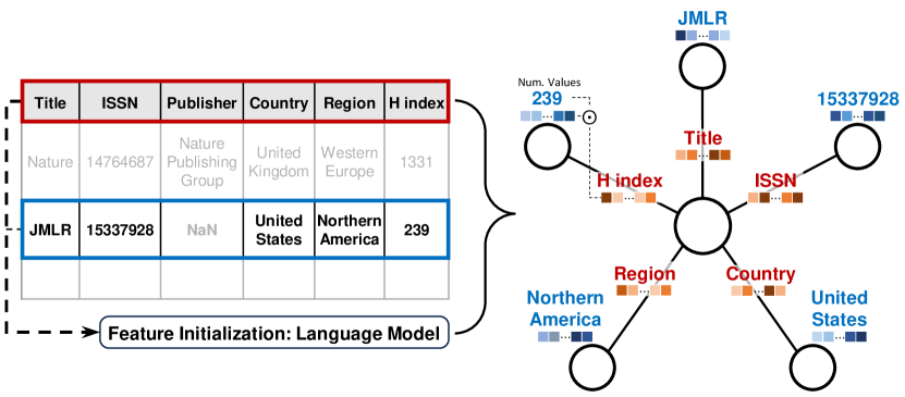
There are several important aspects to be addressed. First, for tabular data, the context of an instance cannot be interpreted fully with the column names. In Figure 1, for example, it would be difficult to grasp the row (blue-box) only with the entries of ‘JMLR’, ‘15337928’, ‘$239$’. The column names ‘Title’, ‘ISSN’, and ‘H index’ clarifies that it is an instance of a journal. CARTE embodies the notion of context in tables through the nodes and edge, which can be exploited by its neural network architecture.

Second, CARTE benefits from the use of language models on non-numerical entries, such as strings, categories, and names. With the language models in feature initialization, the graph transformation in CARTE does not require extensive intervention on discrete entries with data preprocessing or data-cleaning. Moreover, CARTE works with an open set of vocabularies. Problems of typos or wordings of the same meaning, such as ‘North America’ to ‘Northern America’, are readily resolved for CARTE.

This naturally leads to our last point that the proposed graph representation is a powerful representation that can be generalized across heterogeneous tables. The graph transformation with CARTE synchronizes instances from different tables to the same graph domain, without requiring any schema matching for columns or entity matching for entries. Thus, learning process can be operated across many tables, which opens the door for pretraining or transfer.

3.2 Pretrained Model from a Large Knowledgebase

CARTE is pretrained on YAGO3 (Mahdisoltani et al., 2013), a large knowledgebase built from Wikidata and other sources that contain facts about real-world. YAGO stores information as a knowledge graph, which is a collection of triplets (head, relation, tail). For instance, the triplet (Louvre, is located in, Paris) from Figure 2 would be a sample that we can find in YAGO. Our current version of YAGO contains over $18.1$ million triplets of $6.3$ million entities.

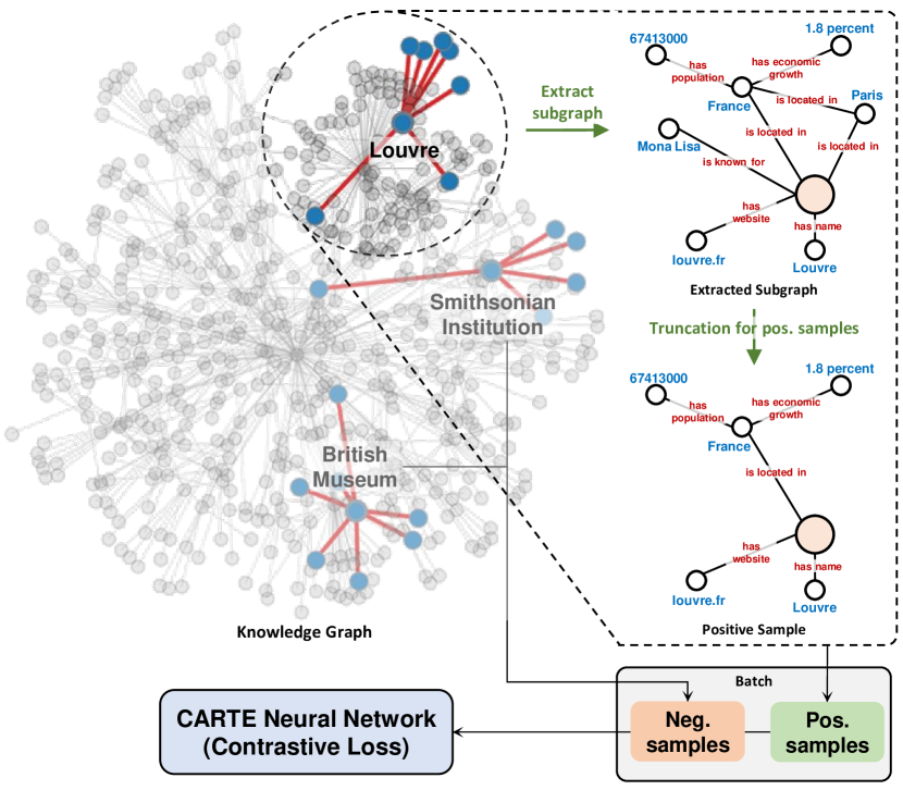
The pretraining process of CARTE can be summarized with Figure 2. From the large knowledge graph, we first extract small graphlets of entities that would work as inputs for CARTE. To enable the self-supervised scheme with a contrastive loss, we also generate truncated versions of selected graphlets and forge them as a batch. Through the training process, CARTE learns how to aggregate information based on the given context. In this subsection, we describe the specific details of the pretraining process.

Figure 2: CARTE pretraining process. From a large knowledge graph, CARTE begins by constructing graphlets and their positives of entities present in YAGO. The extracted samples are then fed into the CARTE neural network and trained with a self-supervised scheme. The resulting neural network learns how to aggregate information within the graphlets, which reflect how table entities can combine entries through the edges (columns)

Graphlets for pretraining

From the large knowledge graph of YAGO, we construct small graphlets of the entities that can be used as inputs for CARTE. To construct a suitable graphlet for an entity, we first extract its subgraph within a user-specified $k$-hop relations. To resemble the structure outlined in Figure 1, while benefiting from additional information through multiple hops, we set $k=2$ with a restriction in the maximum number of $1$-hop and $2$-hop relations as $100$ and $10$, respectively. However, unlike the graph structure shown in Figure 1 the center node would be the name of the entity (for instance ‘Louvre’). To account for the difference, we create an additional neighbor which is comprised of the name as its node and ‘has name’ as its relation. Finally, we initialize node and edge features with the procedure outlined in subsection 3.1 with the FastText embeddings (Mikolov et al., 2017) as the language model.

Batch samples

To construct a batch sample of $N_{b}$, we first select which of the YOGO entities to be included in the batch as graphlets. For this, we employ a selection criteria where $0.9$ of $N_{b}$ are sampled from entities with $6$ or more $1$-hop relations and the remaining $0.1$ from the other subset. The main reason for such sampling scheme is that a large portion of entities in YAGO only have one or two $1$-hop relations, which seldomly come across for tabular data. Moreover, the value $6$ was selected so that the rough median of $1$-hop relations in the batch samples is $15$. To enable the self-supervised contrastive loss, we include positive samples, which are simply the truncation of original graphlets. Through the process, a random fraction (varying from $0.3$ to $0.7$) of the edges were deleted. An exemplary graphlet of ‘Louvre’ and its positive is shown in Figure 2.

Model architecture

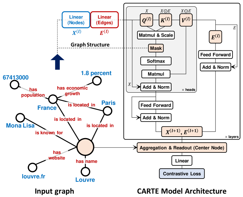
Figure 3 depicts the model structure of CARTE. At its basis, CARTE takes the classical Transformer encoder model in Vaswani et al. (2017), and adapts to a graph attentional network. The key component in CARTE’s architecture is the self-attention layer where both the node and edge features are considered in calculating the attention. The term ‘attention’ in the graph domain refers to the importance of neighbors from a specific node of interest (Velickovic et al., 2017). For graph representation of table entities, the attention translates to the importance of the entries for a given instance with the context supplemented by the column information.

Next, we provide some mathematical details to see how CARTE leverages the the context for the self-attention mechanism. To bring some consistency in notations, we write vectors with an arrow on top $\vec{A}$, matrices in bold $\mathbf{A}$, and scalars $A$. For the ease of reading, we present the case of single-head attention layer, but keep in mind that it can easily be extended to the multi-head schemes of concatenating or averaging the attention outputs.

For a graph with $N$ nodes, let $\vec{X}^{(l)}_{i}\in\mathbb{R}^{d}$ denote the feature of node $i$ and $\vec{E}^{(l)}_{ij}\in\mathbb{R}^{d}$ the feature of the edge directed from node $j$ to $i$. By design, graphlets for CARTE always holds the center node, which we fix its index at $1$. To obtain the representation from the attention layer, we first need to set query, key, and value, which are crucial elements for taking context into account. For query, it should be the vectors of what we are interested in, which are the nodes. Thus, we take the conventional approach and parameterize it with solely the node information. On the other hand, the key-value pairs should convey the elements that the neighboring nodes can offer. Therefore, we additionally parameterized them with the edge information. Keeping this in mind we set the three components as:

$$\vec{Q}_{i} =\vec{X}^{(l)}_{i}\cdot\mathbf{W_{Q}}$$

$$\vec{K}_{ij} =(\vec{X}^{(l)}_{i}\odot\vec{E}^{(l)}_{ij})\cdot\mathbf{W_{K}}$$

$$\vec{V}_{ij} =(\vec{X}^{(l)}_{i}\odot\vec{E}^{(l)}_{ij})\cdot\mathbf{W_{V}}$$

where $\odot$ denotes the element-wise multiplication and $\mathbf{W_{Q}}$, $\mathbf{W_{K}}$, and $\mathbf{W_{V}}$ are trainable weights that reside on $\mathbb{R}^{d\times d}$. Here, the choice of element-wise product is motivated from a knowledge graph embedding technique in Balazevic et al. (2019); Cvetkov-Iliev et al. (2023). These works showed better performance with element-wise multiplication applied on edge and node features compared to translational operations. Following the scaled dot-product attention with the above three equations, the attention score of node $j$ from node $i$, $A_{ij}$, is derived as:

$$A_{ij}=\frac{\exp{(e_{ij})}}{\sum_{k\in\mathcal{N}_{i}}\exp{(e_{ik})}},\,\,\text{where}\,\,e_{ij}=\frac{\vec{Q}_{i}\cdot\vec{K}_{ij}^{T}}{\sqrt{d}}$$ (1)

where the calculation of $A_{ij}$ only takes the sum with respect to the connected neighbors of node $i$. This corresponds masking step, in which we take the inherent graph structure of the input. Notice that if we only considered the node features in $\vec{V}_{ij}$, then the attention score would only be the dot product (a scaled similarity) of projected word vectors of the entities. In such cases, the network would not be able to distinguish between the two cities, ‘Paris’ in France and ‘Paris’ in Texas. Through the attention layers, the outputs for nodes and edges become:

$$\vec{X}_{i}^{(l+1)} =\sigma_{X}(\sum_{j}A_{ij}\cdot\vec{V}_{ij})$$ (2)

$$\vec{E}_{ij}^{(l+1)} =\sigma_{E}(E^{(l)}_{ij}\cdot\mathbf{W_{E}})$$ (3)

where $\sigma$ denote the appropriate consecutive operations (see Figure 3). Finally, the consequent layers consist of the same attention layer, without the edge update, followed by the readout layer that extracts the representation of the center node ($i=1$). The outputs are then processed for the contrastive loss used in the pretraining. For more information on model specification and training details, please refer to Appendix A.1

Contrastive loss

For the self-supervised contrastive loss, we adapted the framework outlined in Chen et al. (2020b). For CARTE, the original and one truncated graphlets are set as positives while the other graphlets in the batch are considered as negatives. The learning loss is then calculated based on the cosine similarity of the network outputs, accompanied by the InfoNCE loss (Oord et al., 2018).

Figure 3: The model architecture for CARTE The inputs of CARTE are graphs that contain node ($X$) and edge ($E$) features, which are both utilized self-attention layer (shown in grey). The attention layers focus on updating the node features based on the context embodied with the edge information. Moreover, the inherent graph structure of the input is reflected in the masking step. The consequent Aggregate & Readout layer consists of the same attention layer (without the edge update) followed by the extraction of the embedding on the center node. The outputs are then processed for the contrastive loss.

3.3 Fine-tuning for downstream tasks

From the architecture shown in Figure 3, the fine-tuning strategy for CARTE is to take two parts from the pretrained model: the initial layers for nodes and edges (blue and red blocks) and the ‘Aggregation & Readout’ layer. Although such simplification is contrary to conventional fine-tuning approaches, it is a suitable one in the view of graph-neural networks. Recall that the graph of downstream table entities would be star-like graphs (Figure 1). Given that the downstream tables contain less variability in graph structures and the cardinality of discrete variables compared to YAGO, the latent representations after each attention layer would lose discriminant characteristics (also known as the over-smoothing problem, Chen et al., 2020a; Rusch et al., 2023, which we study in appendix C.1). Therefore, we take the widely used convention of setting the number of attention layers as the maximum $k$-hop relation, which corresponds to $k=1$. For the final classifier, we simply attach the linear layers. With the base model for fine-tuning, we consider two different settings of downstream inference.

Inference on single tables

This is the well-known setting in which we are given a single table with a target variable to predict. Before transforming table entities into graphs, we preprocess numerical variables with a power transform (Yeo & Johnson, 2000). The power transform has shown to be effective in several works (e.g. Hollmann et al., 2023; Cvetkov-Iliev et al., 2022), and likewise, gives stability to the fine-tuning process of CARTE. Moreover we employ a bagging strategy (Breiman, 1996), in which different models, based on different train-validation splits used for early-stopping, are trained. The prediction outputs are calculated as the average of the outputs from each model.

Transfer from one source table to a target

We also use CARTE in transfer learning setting where we are given a source table $X_{S}$ that can aid predictions on our target table $X_{T}$. Importantly, the source table may have many more samples than the target. We fine-tune CARTE on both tables jointly. Note that the graph representation of the tables enables such joint fine tuning without correspondences in the columns; however, we do need to have similar outcomes $y_{S}$ and $y_{T}$ on both tables. The source outcomes $y_{S}$ are transformed to match the first moment of the target outcome $y_{T}$ using as above a power transform (Yeo & Johnson, 2000, note that here we use the inverse transform). If the target and source table differ on the classification / regression nature of the outcome, we adapt $y_{S}$ as the following: for a classification target $y_{T}$ we binarize regression outcomes in the source table, and for the target regression $y_{T}$, we use binary classification outcomes of the source table, encoded as $\{0,1\}$ and standard scaled. We then proceed to fine tune CARTE by drawing a batch with a fixed proportion of rows from the target and the source table (we use a batch size of 64, 8 of which come from the target). As we consider the settings in which the target table has much fewer samples than the source table, we iterate many more times on the target table, but do early stopping on a validation set of the target table. Note that as in the single-table case, we use a bagging strategy of building multiple learners on different random validation sets and averaging the predictions. Often, early stopping kicks in before all the data points of the source have been covered. This prevents overfitting the source data, which may be less important than the target data for predicting $y_{T}$. Moreover, we use the hyperparameters that have been selected above for the single-table setting.

As we choose source tables quite loosely from weakly-related data, the resulting pair-wise learner may not actually improve upon the single-table learner if the source table does not bring in enough related information. We thus combine the pair-wise learner with the single-table learner ensembling the predictors by combining their output with a softmax. The weights of the softmax are computed using the prediction score computed in the internal validation set of these learners, but divided by the standard deviation across the learners to set the temperature of the softmax.

Joint learning across multiple tables

The key to transfer learning, as above, is finding the right source table. If we have multiple tables from a given domain or institution, CARTE can be adapted to use them all, finding the most useful information for transfer. In these settings we are given a target table $X_{T}$ and a set of source tables ${X_{S,1}...X_{S,m}}$. We proceed to build individual learners: first the single-table learner on $X_{T}$, then each pair of one source table $X_{S,i}$ and the target table $X_{T}$ using the pair-wise joint learner described above. Here again, not every pair-wise learning brings the same amount of useful information. Thus, to find the optimal combination of datasets, we use the same strategy as above of ensembling all the pair-wise predictors as well as the single-table predictor. As a consequence, if all source tables lead to predictors that work as well, they are combined with equal weights, but if one source dominates, the prediction is anchored on this one.

4 Experimental study

4.1 Experimental setup

Datasets

We used 51 tabular learning datasets, all with an associated learning task –40 regressions and 11 classification–, gathered across multiple sources, mainly from previous machine learning studies and kaggle competitions. These datasets cover a variety of topics of society and businesses: accidents, elections, remunerations, food, restaurants, etc. We select datasets that were representative of modern data science applications: tabular data with meaningful columns and discrete entries, unlike many datasets from UCI . Appendix B gives the specific list of datasets.

Baselines

We evaluate different baselines, with the following abbreviations (details and hyper-parameter tuning in Appendix A.2):

TabVec-…-HGB,

a family of baselines using the TableVectorizer from the Skrub package (Skrub, 2024) to encode tables into numerical arrays. When applied on all features (TabVec-HGB), text features are encoded using the Gamma-Poisson encoder from skrub, introduced in Cerda & Varoquaux (2022), which extracts latent categories from substrings. We also use tailored strategy to encode columns that we manually identify as containing rich strings or entity names. For this the corresponding columns are encoded either with FastText (Joulin et al., 2017) (TabVec-FT-HGB) or with an LLM –we use intfloat/e5-small-v2 (Wang et al., 2022) from HuggingFace– (TabVec-FT-LLM, and the TableVectorizer is applied on remaining numerical and categorical features. For all these baselines, the encoded table is passed into the HistGradientBoosting estimators from scikit-learn (Pedregosa et al., 2011).

CatBoost

(Dorogush et al., 2018), a gradient-boosted trees package commonly used to learn on tables. We treat text features as categorical, which are encoded by CatBoost’s categorical encoding, an improved version of target encoding (Micci-Barreca, 2001).

S-LLM

Inspired by TabLLM (Hegselmann et al., 2023), we investigate encoding each row of a table with an LLM. We represent each row as a sentence, alternate the column names and the corresponding entries, and encode the table with the last hidden layer. Unlike TabLLM, however, the encoded table is passed to the HistGradientBoosting estimator as this led to better prediction accuracies. The benefit of using an LLM is that, as with CARTE, it gives a consistent representation of data without requiring correspondences in columns. For numerical entries, we investigate either concatenating them as additional features outside of the LLM (CN), or passing them as strings to the LLM (EN).

MLP

The classical Multilayer Perceptron with target encoder (Micci-Barreca, 2001) for treating categorical features. The missing values were imputed with the mean for numerical features, while they were treated as another category for categorical features. After the transformations, we applied the minmax scale on all columns to set the values in between zero and one.

Resnet

Similar architecture to the MLP (with the same encoding and transformation measures), but with additional layernorm/batchnorm and skip-connections.

TabPFN

(Hollmann et al., 2023) is a transformer model pretrained on synthetic data to generate predictions for new (small) datasets in one forward pass. We treat the text features as categorical and encode them with a target encoder (Micci-Barreca, 2001).

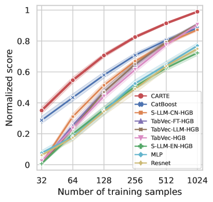
a. Regression – 40 datasets HGB = sklearn’s HistGradientBoosting
TabVec = skrub’s TableVectorizer
FT = FastText
CN = concat numerical
EN = embed numerical 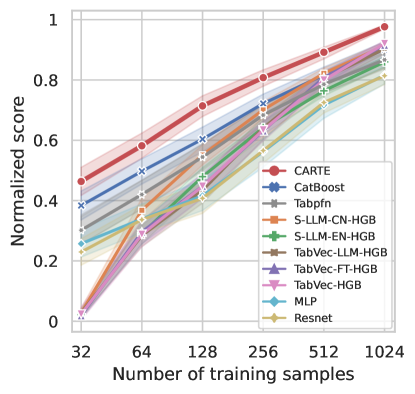                                                                 b. Classification – 11 datasets

Figure 4: CARTE outperforms alternatives for learning on single tables. Learning curve on (a) regression and (b) classification tasks over 51 datasets. Top: normalized score (for a given dataset, 1 is the best performing score across all methods and training-set size, and 0 is the worst), averaged across all datasets. Bottom: critical difference diagrams, for $n=1024$ (code from Ismail Fawaz et al., 2019).

4.2 Results on single tables

CARTE outperforms alternatives for learning on single tables

Figure 4 compares the prediction performance of the multiple methods, summarizing the different datasets. We see that CARTE consistently outperforms alternatives across the different sample sizes, whether it is with normalized score or critical difference diagrams based on the Wilcoxon-Holm method to detect pairwise significance.

Entity matching not required for CARTE

The hypothesis to explain the good performance of CARTE is that has integrated information on many entities because it has been pretrained on the YAGO knowledge base. However, in a given downstream table, entities might appear written in a different way: for instance ”Londres” instead of ”London”. This begs the question of whether CARTE transfers well useful information if the string representation of the entities differs. String matching is necessary for instance when using as features vector embeddings of the entries such as KEN embeddings (Cvetkov-Iliev et al., 2023).

Figure 5: Entity matching not required for CARTE, and downstream entities do not need in YAGO to work. We evaluate CARTE and KEN either on the full datasets, or on a reduced version of the datasets corresponding to entities present in YAGO. In addition, when entities are present in YAGO, we compare matching them to their canonical name in YAGO (blue) or leaving the original names (orange). When KEN is used enrich the dataset, CatBoost is used for prediction, and entities without match are replaced with missing values. Each point on the figure correspond to an improvement in performance with respect to Catboost without any enrichment for a dataset and a training size. Detailed results in Appendix C.2.

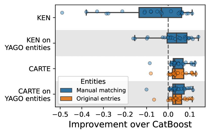
On four of our datasets (company employees, movies, US accidents, and US election), we performed manual entity matching of the entries to their corresponding YAGO entity. Figure 5 shows that while using KEN requires entity matching to have good performance, CARTE has string-level models, and its performance does not vary between using original entries or manually matched entities.

4.3 Learning across multiple tables

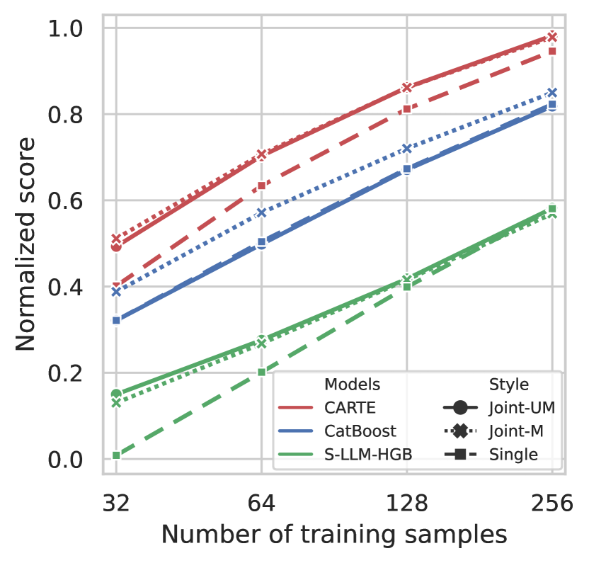
Joint learning 84 cases of two tables                                                                                   HGB = sklearn’s HistGradientBoosting
UM = columns unmatched
M = columns matched

Figure 6: Schema matching not required for CARTE, with consistent improvements through joint learning. We compare three scenarios (style) – single (dashed lines): only the target tables; joint (full lines): the automated transfer learning without any manual operation; matched (dotted lines): transfer learning after manually matching the columns.

We investigate learning across multiple tables without explicit correspondences across columns. We use tables “in the wild”: in our 51 datasets, we find groups covering the same general topic (selling bikes, rating restaurants) though they come from different sources (appendix B.3). In this setting, we can readily use CARTE and S-LLM approaches as they use an open-vocabulary representation of the column to embed entries (but only the EN, Embed Numerical, version of S-LLM, as the CN, Concat Numerical, needs correspondence for the numerical columns). As CatBoost natively deals with missing values, we use it by concatenating the datasets and adding missing values for columns that mismatch. We also investigate manual matching of columns.

Schema matching not required for CARTE

Figure 6 shows results for transfer learning across only two tables. We see that for all approaches transfer learning can help (the dashed line, representing the learning only on the target table, is below), but only CARTE provides consistent improvements without requiring manual column matching. For CatBoost, the matching (dotted line) is crucial, which is not the case for the other approaches. For S-LLM, the benefit of transfer drops rapidly with respect to the number of training samples. The results show that CARTE does not need schema matching, and it provides consistent improvements in the target table with transfer. Extended results of schema-matching can be found in Appendix C.3.

Figure 7: CARTE further benefits from additional source tables. Each point represents an average increase in the performance of CARTE on a target table from the case of no source tables, when incorporating different number of sources into its training process. For each setting, we permute the tables so that each table is used both as target and as source.

Joint learning from multiple tables

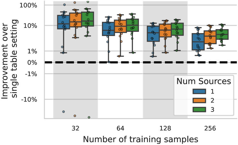
The difficulty for transfer learning may be finding good source tables. In Figure 7, we investigate bringing in more source tables, up to a total of 4 tables (1 target, and 3 sources, with a total of 245 cases). CARTE benefits from adding source tables: not only does the median performance improve but also, the variability with respect the lower range improves quickly. In other words, with more source tables, there are more chances of finding a real beneficial one, and thus the worst-case scenario becomes better.

5 Conclusion

By using an architecture that models table entries not as a $i^{\text{th}}$ feature in a data matrix but as a function of its context (column names and neighboring entries) as well open-vocabulary embedding of strings, CARTE enables consistent representations of very different tabular data. This opens the door to pre-training across background tables, and fine-tuning to downstream tasks without need for entity or schema matching. Our results show that after pretraining on a large knowledge base, the resulting model brings marked benefits to downstream analytic tasks, consistently outperforming a broad range of baselines both for learning on a single table or transfer learning on tables with imperfect correspondences. It enables transfer from tables in the wild, a setting so far never studied. Pre-training has been key to the wide application of deep learning on images and text. We hope that the ideas behind CARTE will bring these benefits to tabular learning, enabling further improved architectures, for instance by merging with the complementary meta-learning ideas of TabPFN (Hollmann et al., 2023).

Appendix A Detailed information on training

A.1 Pretrained model of CARTE

Model specification and training details

The model specification and training details were largely referenced from the work of Devlin et al. (2019). We set $12$ attention layers, each consisting of $12$ multi-head attentions, and the hidden dimension was fixed to the same size as the inputs ($300$). The resulting model contains over $9.3$ million parameters. To run the pretraining, we selected $128$ entities with one additional positive, resulting in the batch size of $256$. The total number of steps for training was $1,000,000$, which approximately covers $40$ epochs with respect to YAGO entities. We use the AdamW optimizer accompanied by the cosine scheduler with $lr_{min}=5\times 10^{-6}$, $lr_{max}=1\times 10^{-4}$ and a warmup over the first $10,000$ steps. The dropout rate was fixed to $0.1$ and the gelu activation function was used.

A.2 Details on experiment settings for downstream tasks

Single tables

To evaluate the performances of baselines on single tables, we focused on the few-shot learning setting with the number of train data for each table varying from $32$, $64$, $128$, $256$, $512$, and $1,024$; the rest of the remaining data were set as the test set. To find the optimal hyperparameters of the baselines, $5$-fold cross-validation over $100$ random search iteration were carried out on all the comparing methods except for CARTE and TabPFN. For CARTE, the same $5$-fold cross-validation, but only the grid-search over the learning rate was conducted. For Tabpfn, we ran with the default values, as suggested in the paper. For detailed information the hyperparameter spaces of each method, please refer to the Hyperparmeter tuning paragraph below. The performance was recorded on $10$ different train/test splits, with the performance measure set as the $R^{2}$ score for regression tasks and the Area Under Receiver Operating Curve (AUROC) for classification tasks.

Joint learning across multiple tables

The experiment settings for joint learning is almost the same as in the single table setting, except for minor details. The number of train-set on the target was varied across $32$, $64$, $128$, $256$, while the same split was set as in the case of single-tables to make the results comparable. In terms of hyperparameter optimization, CARTE only takes the best values obtained from the the single-table case (section 3). For other baselines, the same scheme for hyperparameter search was conducted.

Hyperparameter space

The hyperparameter tuning was done using grid search for CARTE, as we only tune the learning rate, and with random search for the baselines as these come with more than two hyperparameters to tune. The hyperparmeter spaces for the HGB, Resnet, and MLP baselines are based on that used in Grinsztajn et al. (2022); for CatBoost we follow that used in the CatBoost paper (Dorogush et al., 2018). For the baselines in joint learning across multiple tables, we employ an additional hyperparameter ‘fraction source’, which denote the fraction of source data used for training. The tables below depict the hyperparameter spaces for each.

Parameter	Grid
Learning rate	[$2.5$, $5$, $7.5$] $\times$ [$1e^{-4}$, $1e^{-3}$]

Table 1: CARTE hyperparameter space

Parameter	Distribution
Max depth	UniformInt [$2$, $6$]
Learning rate	LogUniform [$1e^{-5}$, $1$]
Bagging temperature	Uniform [$0$, $1$]
$l_{2}$-leaf regularization	LogUniform [$1$, $10$]
Random strength	UniformInt [$1$, $2$]
One hot max size	UniformInt [$2$, $25$]
Iterations	UniformInt [$400$, $1000$]

Table 2: CatBoost hyperparameter space, adapted from Dorogush et al. (2018)

Parameter	Distribution
Learning rate	LogUniform [$1e^{-2}$, $10$]
Max depth	[None, $2$, $3$, $4$]
Max leaf nodes	NormalInt [$31$, $5$]
Min samples leaf	NormalInt [$20$, $2$]
$l_{2}$-regularization	LogUniform [$1e^{-6}$, $1e^{3}$]

Table 3: HistGradientBoosting hyperparameter space, adapted from Grinsztajn et al. (2022)

Parameter	Distribution
Num layers	UniformInt [$1$, $8$]
Layer size	UniformInt [$32$, $512$]
Hidden factor	UniformInt [$1$, $3$]
Hidden dropout	Uniform [$0$, $0.5$]
Residual dropout	Uniform [$0$, $0.5$]
Learning rate	LogUniform [$1e^{-5}$, $1e^{-2}$]
Weight decay	LogUniform [$1e^{-8}$, $1e^{-2}$]
Normalization	[batchnorm, layernorm]
Batch size	[$16$, $32$]

Table 4: Resnet hyperparameter space, adapted from Grinsztajn et al. (2022)

Parameter	Distribution
Num layers	UniformInt [$1$, $4$]
Layer size	UniformInt [$16$, $1024$]
Dropout	Uniform [$0$, $0.5$]
Learning rate	LogUniform [$1e^{-5}$, $1e^{-2}$]
Weight decay	LogUniform [$1e^{-8}$, $1e^{-2}$]
Batch size	[$16$, $32$]

Table 5: MLP hyperparameter space, adapted from Grinsztajn et al. (2022)

Parameter	Distribution
Source fraction	Uniform [$0$, $1$]

Table 6: Additional hyperparameter for the baselines in joint learning

Appendix B Data Description

B.1 Data proprocessing

Only minimal data preprocessing were carried out in data preparation. For all datasets, we excluded columns that contained only one unique value or had missing values over half the size of the dataset.

B.2 Datasets used

We provide detailed description of the datasets used in our experiment study.

1. Anime Planet This dataset contains information about anime scrapped from the website Anime-Planet. The task is to predict the average rating of the anime on this site.

2. Babies R Us (Sanjib et al., 2023) Information of baby products scraped from the Babies R Us website. The task is to predict the price of baby products.

3. Buy Buy Baby (Sanjib et al., 2023) Information of baby products scraped from the Buy Buy Baby website. The task is to predict the price of baby products.

4. Beer Ratings : The dataset contains tasting profiles and consumer reviews for 3197 unique beers from 934 different breweries. The task is to predict overall review ratings of different beers.

5. Bikedekho (Sanjib et al., 2023) Information on bikes and scooters from bikedekho website in India. The task is to predict the price of bikes.

6. Bikewale (Sanjib et al., 2023) Information on bikes and scooters from bikewale website in India. The task is to predict the price of bikes.

7. Cardekho . This dataset contains information on used cars, with their listing price in the websit Cardekho. The task is to predict the price.

8. Chocolate Bar Ratings .Dataset containing information and expert rating on cocoa batches. The task is to predict the rating.

9. Clear Corpus (Crossley et al., 2023): Generic information about the reading passage excerpts for elementary school students. The task is to predict the readability of the excerpts. The text feature is the name of the book, not the excerpt.

10. Coffee Ratings Dataset scraped from coffeereview.com containing information on various coffees. The task is to predict the review ratings of the coffees.

11. Company Employees: Information on companies with over $1,000$ employees. The task is to predict the number of employees of each company.

12. Employee remuneration and expenses earning over 75000 Remuneration and expenses for employees earning over $75,000 per year. The task is to predict the remuneration of employees.

13. Employee Salaries : Information on salaries for employees of the Montgomery County, MD. The task is to predict the current annual salary range of the employees.

14. Fifa22 Players : Information on soccer players and their ability scores in Fifa22 game. The task is to predict the player’s wage.

15. Filmtv Movies : Information of movies and ratings scraped from an Italian movie review website Filmtv Movies. The task is to predict the public vote on movies.

16. Journal Score JCR: Scientific journals and their descriptive features from Journal Citation Reports. The task is to predict the impact factors of the journals.

17. Journal Score SJR: Scientific journals and their descriptive features from Scimago journal rank. The task is to predict the H-index of journals.

18. Japanese Anime: : List of Japanese animes and their relevant information. The task is to predict score for the animes.

19. K-Drama: : List of korean drama and their basic information from mydramalist website. The task is to predict the score of the korean dramas.

20. Michelin: : List of restaurants along with additional details curated from the Michelin Restaurants guide. The task is to predict the award of the restaurants.

21. ML/DS Salaries: salary and basic information of workers in machine learning and data science industry. The task is to predict the salary of workers.

22. Movie Revenues: : Metadata of movies released on or before July 2017. The task is to predict the range of the box-office revenues.

23. Museums: : General information on the US museums. The task is to predict the revenues across the museums.

24. Mydramalist: General information on Asian drama scaped from mydramalist website. The task is to predict the ratings of Asian dramas.

25. NBA Draft: Information on all NBA Draft picks from 1989-2021. The task is to predict the ‘value over replacement’ of players.

26. Prescription Drugs: The data contains new prescription drugs introduced to market in California with a Wholesale Acquisition Cost (WAC) that exceeding Medicare Part D. The task is to predict WAC at introduction.

27. Ramen ratings. The dataset contains ratings and characteristics of various ramens produced from multiple countries. The task is to predict the range of ratings of the ramens.

28. Roger Ebert:. The dataset contains movies ratings by famous critic Rogert Ebert. The task is to predict the range of ratings.

29. Rotten Tomatoes:(Sanjib et al., 2023) . Contain information on movies that can be found in Rotten Tomatoes movie rating website. The task is to predict the rating values of the movies.

30. Spotify: Generic information on Spotify tracks with some associated audio features. The task is to predict the popularity of the albums.

31. US Accidents: Information of accidents in US cities between 2016 and 2020. From this dataset, two tasks are conducted: (1) the range of accident counts for the US cities (2) the severity of the reported accidents.

32. US Presidential (Cvetkov-Iliev et al., 2022): Voting statistics in the 2020 US presidential election along with information on US counties. The task is to predict the range of voting numbers across US counties.

33. Used Cars 24: . Information on used cars. The task is to predict the price.

34. Used Cars Benz Italy: Dataset containing information on used cars sold in Italy. The task is to predict the price.

35. UsedCars.com: Dataset containing information on used cars usedcars.com. The task is to predict the price.

36. Used Cars Pakistan: . Dataset containing information on used cars sold in Pakistan. The task is to predict the price.

37. Used Cars Saudi Arabia: Dataset containing information on used cars sold in Saudi Arabia from the Syarah Website. The task is to predict the price of used cars.

38. Videogame Sales: This dataset contains a list of video games with sales greater than 100,000 copies (scrape of vgchartz.com). The task is to predict the global sales of the videogames.

39. Whisky: Basic and tasting information on whiskies form the whiskyanalysis.com. The task is to predict the range of meta critic of the whiskies.

40. Wikiliq: Information on alcohol that can be found in the Wikiliq website. We conducted two tasks to predict the prices of (1) beer and (2) spirits.

41. Wina Poland: Information about wines on the polish market. The task is to predict the price.

42. Wine.com: Information on wines scraped from the wine.com website. We conducted two tasks on prediction of (1) wine ratings and (2) wine prices.

43. WineEnthusiasts: Information about a wine and a taster from winemag.com. We conducted two tasks on prediction of (1) wine ratings and (2) wine prices.

44. WineVivino: . Information about wine bottles scrapped from Vivino’s website. We conducted two tasks on prediction of (1) wine ratings and (2) wine prices.

45. Yelp: The Yelp Open dataset for academic research. We extracted information on the restaurants from the original dataset. The task is to predict the range of stars for the restaurants. https://www.yelp.com/dataset

46. Zomato. Information and reviews of restaurants found in the zomato websites. The task is to predict the range of ratings for each restaurants.

B.3 Datasets from multi-table experiments

For the multi-table experiments we extract from the list above groups of tables that are related to the same topics:

Wine prices

: Wina Poland, WineEnthusiasts, WineVivino, Wine.com

Wine ratings

: WineEnthusiasts, WineVivino, Wine.com

Beers

: Beer Ratings, Wikiliq-Beer

Used Cars

Used Cars 24, Used Cars Benz Italy, UsedCars.com, Used Cars Pakistan, Used Cars Saudi Arabia

Films

Filmtv Movies, Rotten Tomatoes

Dramas

K-Drama, Mydramalist

Animes

Anime Planet, Japanese Anime

Baby products

Buy Buy Baby, Babies R Us

Bike sales

Bikedekho, Bikewale

Employee remunerations

Company Employees, Employee remuneration and expenses earning over 75000, ML/DS Salaries

Restaurant ratings

Zomato, Michelin, Yelp

Journal scores

Journal Score JCR, Journal Score SJR

Appendix C Extended results

C.1 The effect of oversmoothing

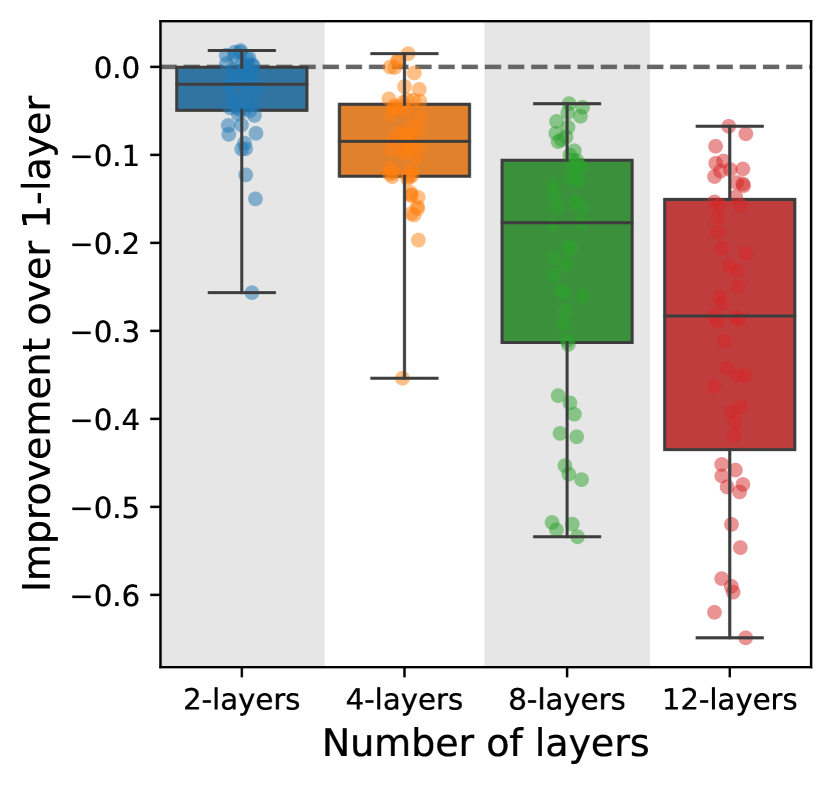
Figure 8 show that representations extracted from deeper layers of the Graph Neural Networks (GNNs) are less useful for prediction on downstream tasks. We interpret this as an effect of oversmoothing, a well known problem in GNNs (Chen et al., 2020a; Rusch et al., 2023).

Figure 8: The effect of oversmoothing: comparing prediction from representations extracted from the GNN from the 2^nd, 4^th, 8^th, and 12^th layers, with that build from the first layer. We see that the deeper we go in the GNN, the less useful the representation is for downstream task. We interpret this as an effect of oversmoothing.

C.2 Details of the entity matching experiment

The experiments were conducted with the same experiment settings as that of the singletable experiments. Table 7 gives the specific results behind each dataset used in the entity matching experiment Figure 5. The specific datasets are

• CE = Company employees : 32% of the companies matched to YAGO

• MV = movie revenues : 84% of the movies matched to YAGO

• US-Acc = US accidents : 67% of the cities matched to YAGO

• US-Elec = US elections : 98% of the counties matched to YAGO

	CatBoost-MR	CatBoost-MF	CatBoost-OR	CatBoost-OF
CE-32	0.673$\pm$0.036	0.672$\pm$0.063	0.683$\pm$0.052	0.668$\pm$0.062
CE-64	0.707$\pm$0.021	0.72$\pm$0.013	0.702$\pm$0.025	0.718$\pm$0.017
CE-128	0.734$\pm$0.007	0.739$\pm$0.024	0.731$\pm$0.011	0.745$\pm$0.01
CE-256	0.739$\pm$0.008	0.747$\pm$0.014	0.74$\pm$0.009	0.749$\pm$0.008
CE-512	0.744$\pm$0.005	0.758$\pm$0.005	0.744$\pm$0.005	0.758$\pm$0.004
CE-1024	0.752$\pm$0.006	0.763$\pm$0.004	0.752$\pm$0.006	0.764$\pm$0.003
MV-32	0.4$\pm$0.058	0.398$\pm$0.049	0.394$\pm$0.058	0.403$\pm$0.042
MV-64	0.436$\pm$0.043	0.449$\pm$0.045	0.426$\pm$0.059	0.453$\pm$0.035
MV-128	0.484$\pm$0.027	0.492$\pm$0.028	0.482$\pm$0.018	0.495$\pm$0.019
MV-256	0.511$\pm$0.011	0.515$\pm$0.017	0.51$\pm$0.017	0.523$\pm$0.012
MV-512	0.545$\pm$0.007	0.55$\pm$0.007	0.545$\pm$0.009	0.552$\pm$0.008
MV-1024	0.559$\pm$0.007	0.574$\pm$0.007	0.563$\pm$0.005	0.573$\pm$0.005
US-Acc-32	-0.016$\pm$0.063	-0.018$\pm$0.064	-0.023$\pm$0.076	-0.02$\pm$0.058
US-Acc-64	0.007$\pm$0.055	-0.01$\pm$0.069	0.028$\pm$0.036	-0.023$\pm$0.087
US-Acc-128	0.082$\pm$0.026	0.055$\pm$0.029	0.084$\pm$0.028	0.057$\pm$0.026
US-Acc-256	0.129$\pm$0.018	0.089$\pm$0.031	0.129$\pm$0.015	0.089$\pm$0.025
US-Acc-512	0.163$\pm$0.02	0.12$\pm$0.022	0.163$\pm$0.021	0.121$\pm$0.02
US-Acc-1024	0.214$\pm$0.007	0.157$\pm$0.01	0.217$\pm$0.005	0.155$\pm$0.009
US-Elec-32	0.31$\pm$0.133	0.318$\pm$0.142	0.34$\pm$0.118	0.285$\pm$0.161
US-Elec-64	0.433$\pm$0.062	0.441$\pm$0.068	0.449$\pm$0.038	0.445$\pm$0.056
US-Elec-128	0.512$\pm$0.019	0.505$\pm$0.02	0.511$\pm$0.02	0.51$\pm$0.02
US-Elec-256	0.547$\pm$0.009	0.543$\pm$0.011	0.546$\pm$0.009	0.544$\pm$0.011
US-Elec-512	0.572$\pm$0.007	0.571$\pm$0.01	0.57$\pm$0.009	0.571$\pm$0.008
US-Elec-1024	0.586$\pm$0.004	0.586$\pm$0.006	0.586$\pm$0.005	0.587$\pm$0.005

	CARTE-MR	CARTE-MF	CARTE-OR	CARTE-OF	KEN-R	KEN-F
CE-32	0.699$\pm$0.023	0.69$\pm$0.034	0.693$\pm$0.023	0.692$\pm$0.029	0.518$\pm$0.11	0.459$\pm$0.119
CE-64	0.729$\pm$0.019	0.744$\pm$0.025	0.733$\pm$0.01	0.747$\pm$0.022	0.612$\pm$0.077	0.434$\pm$0.284
CE-128	0.755$\pm$0.007	0.763$\pm$0.012	0.755$\pm$0.01	0.763$\pm$0.014	0.708$\pm$0.019	0.409$\pm$0.305
CE-256	0.762$\pm$0.009	0.776$\pm$0.01	0.763$\pm$0.008	0.781$\pm$0.007	0.738$\pm$0.02	0.368$\pm$0.812
CE-512	0.773$\pm$0.011	0.785$\pm$0.007	0.778$\pm$0.012	0.789$\pm$0.008	0.757$\pm$0.006	0.267$\pm$0.494
CE-1024	0.783$\pm$0.008	0.793$\pm$0.006	0.787$\pm$0.01	0.798$\pm$0.006	0.772$\pm$0.008	0.486$\pm$0.301
MV-32	0.3$\pm$0.057	0.313$\pm$0.083	0.329$\pm$0.066	0.322$\pm$0.095	0.301$\pm$0.057	0.318$\pm$0.033
MV-64	0.452$\pm$0.044	0.471$\pm$0.027	0.458$\pm$0.025	0.461$\pm$0.038	0.42$\pm$0.035	0.369$\pm$0.055
MV-128	0.521$\pm$0.022	0.523$\pm$0.022	0.519$\pm$0.023	0.515$\pm$0.018	0.493$\pm$0.024	0.384$\pm$0.08
MV-256	0.556$\pm$0.022	0.562$\pm$0.02	0.554$\pm$0.021	0.555$\pm$0.014	0.543$\pm$0.014	0.464$\pm$0.089
MV-512	0.594$\pm$0.013	0.597$\pm$0.013	0.595$\pm$0.014	0.595$\pm$0.011	0.589$\pm$0.012	0.517$\pm$0.04
MV-1024	0.62$\pm$0.008	0.622$\pm$0.008	0.62$\pm$0.008	0.618$\pm$0.009	0.616$\pm$0.007	0.544$\pm$0.032
US-Acc-32	0.061$\pm$0.054	0.053$\pm$0.055	0.054$\pm$0.067	0.048$\pm$0.045	0.062$\pm$0.094	0.047$\pm$0.045
US-Acc-64	0.112$\pm$0.057	0.114$\pm$0.046	0.122$\pm$0.056	0.105$\pm$0.051	0.146$\pm$0.038	0.051$\pm$0.09
US-Acc-128	0.155$\pm$0.06	0.136$\pm$0.053	0.16$\pm$0.058	0.14$\pm$0.051	0.175$\pm$0.025	0.117$\pm$0.026
US-Acc-256	0.225$\pm$0.024	0.197$\pm$0.023	0.232$\pm$0.02	0.2$\pm$0.024	0.225$\pm$0.029	0.152$\pm$0.014
US-Acc-512	0.278$\pm$0.008	0.237$\pm$0.01	0.275$\pm$0.015	0.235$\pm$0.014	0.27$\pm$0.012	0.173$\pm$0.029
US-Acc-1024	0.303$\pm$0.01	0.263$\pm$0.008	0.304$\pm$0.008	0.265$\pm$0.012	0.298$\pm$0.004	0.205$\pm$0.006
US-Elec-32	0.387$\pm$0.082	0.387$\pm$0.083	0.393$\pm$0.08	0.393$\pm$0.082	0.149$\pm$0.193	0.209$\pm$0.159
US-Elec-64	0.467$\pm$0.031	0.467$\pm$0.032	0.465$\pm$0.021	0.465$\pm$0.022	0.432$\pm$0.089	0.454$\pm$0.073
US-Elec-128	0.52$\pm$0.021	0.52$\pm$0.021	0.52$\pm$0.022	0.52$\pm$0.022	0.564$\pm$0.038	0.571$\pm$0.035
US-Elec-256	0.552$\pm$0.011	0.553$\pm$0.011	0.546$\pm$0.013	0.546$\pm$0.013	0.625$\pm$0.019	0.628$\pm$0.011
US-Elec-512	0.586$\pm$0.008	0.586$\pm$0.008	0.58$\pm$0.007	0.581$\pm$0.007	0.667$\pm$0.006	0.664$\pm$0.01
US-Elec-1024	0.615$\pm$0.007	0.615$\pm$0.007	0.612$\pm$0.007	0.613$\pm$0.007	0.7$\pm$0.009	0.697$\pm$0.005

Table 7: Detailed results of the entity matching experiment: individual scores on each dataset. The abbreviations are as follows: O-Original entries, M-Matched entries, R-Reduced dataset, and F-Full dataset.

C.3 Schema-matching results on joint learning across multiple tables

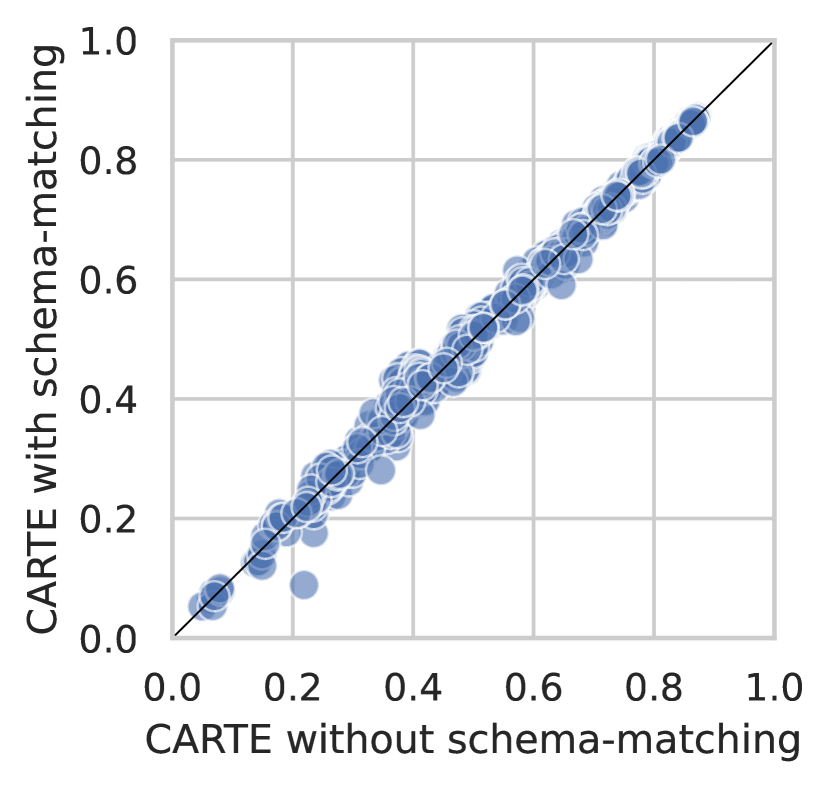
Figure 9 depicts a direct comparison of performance between CARTE with and without schema-matching over 275 different cases in number of source data (ranging from one source to five sources). Each point represents a comparison of the average score over a dataset with different train/test split for a given size of train data. If a point is located below the diagonal line, it indicates a higher performance of x-axis. From the figure, we see that dots align along the diagonal line, indicating similar performance between CARTE with and without schema-matching (also with p-value of 0.728 for two-sided t-test on difference in means). The results suggest schema-matching is not required for CARTE on transfer across multiple tables.

Figure 9: Performance comparison of CARTE with and without schema-matching: The figures portrays a direct comparison of performance between CARTE with and without schema-matching over 275 different cases in number of source data. A point below the diagonal line indicate better performance of the method in x-axis. We see that the dots align along the diagonal line, showing similar performance both approaches of CARTE on joing learning (p-value of 0.728). The results bolster no schema-matching for CARTE.

References

- Abutbul et al. (2020) Abutbul, A., Elidan, G., Katzir, L., and El-Yaniv, R. DNF-Net: A Neural Architecture for Tabular Data, June 2020.
- Arik & Pfister (2020) Arik, S. O. and Pfister, T. TabNet: Attentive Interpretable Tabular Learning, December 2020.
- Balazevic et al. (2019) Balazevic, I., Allen, C., and Hospedales, T. Multi-relational poincaré graph embeddings. Advances in Neural Information Processing Systems, 32, 2019.
- Bommasani et al. (2021) Bommasani, R., Hudson, D. A., Adeli, E., Altman, R., Arora, S., von Arx, S., Bernstein, M. S., Bohg, J., Bosselut, A., Brunskill, E., et al. On the opportunities and risks of foundation models. arXiv preprint arXiv:2108.07258, 2021.
- Breiman (1996) Breiman, L. Bagging predictors. Machine learning, 24:123–140, 1996.
- Cerda & Varoquaux (2022) Cerda, P. and Varoquaux, G. Encoding high-cardinality string categorical variables. IEEE Transactions on Knowledge and Data Engineering, 34(3):1164–1176, March 2022. ISSN 1041-4347, 1558-2191, 2326-3865. doi: 10.1109/TKDE.2020.2992529.
- Chen et al. (2020a) Chen, D., Lin, Y., Li, W., Li, P., Zhou, J., and Sun, X. Measuring and relieving the over-smoothing problem for graph neural networks from the topological view. In Proceedings of the AAAI conference on artificial intelligence, volume 34, pp. 3438–3445, 2020a.
- Chen et al. (2023) Chen, J., Yan, J., Chen, D. Z., and Wu, J. ExcelFormer: A Neural Network Surpassing GBDTs on Tabular Data, January 2023.
- Chen & Guestrin (2016) Chen, T. and Guestrin, C. Xgboost: A scalable tree boosting system. In Proceedings of the 22nd acm sigkdd international conference on knowledge discovery and data mining, pp. 785–794, 2016.
- Chen et al. (2020b) Chen, T., Kornblith, S., Norouzi, M., and Hinton, G. A simple framework for contrastive learning of visual representations. In International conference on machine learning, pp. 1597–1607. PMLR, 2020b.
- Crossley et al. (2023) Crossley, S., Heintz, A., Choi, J. S., Batchelor, J., Karimi, M., and Malatinszky, A. A large-scaled corpus for assessing text readability. Behavior Research Methods, 55(2):491–507, 2023.
- Cvetkov-Iliev et al. (2022) Cvetkov-Iliev, A., Allauzen, A., and Varoquaux, G. Relational Data Embeddings for Feature Enrichment with Background Information. Machine Learning, 112, 2022. doi: 10.1007/s10994-022-06277-7.
- Cvetkov-Iliev et al. (2023) Cvetkov-Iliev, A., Allauzen, A., and Varoquaux, G. Relational data embeddings for feature enrichment with background information. Machine Learning, 112(2):687–720, 2023.
- Deng et al. (2020) Deng, X., Sun, H., Lees, A., Wu, Y., and Yu, C. TURL: Table Understanding through Representation Learning, December 2020.
- Devlin et al. (2019) Devlin, J., Chang, M.-W., Lee, K., and Toutanova, K. BERT: Pre-training of Deep Bidirectional Transformers for Language Understanding, May 2019.
- Doan et al. (2012) Doan, A., Halevy, A., and Ives, Z. Principles of data integration. Elsevier, 2012.
- Dorogush et al. (2018) Dorogush, A. V., Ershov, V., and Gulin, A. CatBoost: Gradient boosting with categorical features support. arXiv preprint arXiv:1810.11363, 2018.
- Eggert et al. (2023) Eggert, G., Huo, K., Biven, M., and Waugh, J. TabLib: A Dataset of 627M Tables with Context, October 2023.
- Gardner et al. (2022) Gardner, J., Popovic, Z., and Schmidt, L. Subgroup Robustness Grows On Trees: An Empirical Baseline Investigation. Advances in Neural Information Processing Systems, 35:9939–9954, December 2022.
- Gorishniy et al. (2023a) Gorishniy, Y., Rubachev, I., Kartashev, N., Shlenskii, D., Kotelnikov, A., and Babenko, A. TabR: Tabular Deep Learning Meets Nearest Neighbors in 2023, October 2023a.
- Gorishniy et al. (2023b) Gorishniy, Y., Rubachev, I., Khrulkov, V., and Babenko, A. Revisiting Deep Learning Models for Tabular Data, October 2023b.
- Grinsztajn et al. (2022) Grinsztajn, L., Oyallon, E., and Varoquaux, G. Why do tree-based models still outperform deep learning on tabular data?, July 2022.
- Hegselmann et al. (2023) Hegselmann, S., Buendia, A., Lang, H., Agrawal, M., Jiang, X., and Sontag, D. TabLLM: Few-shot Classification of Tabular Data with Large Language Models, March 2023.
- Hollmann et al. (2023) Hollmann, N., Müller, S., Eggensperger, K., and Hutter, F. TabPFN: A Transformer That Solves Small Tabular Classification Problems in a Second, September 2023.
- Hulsebos et al. (2019) Hulsebos, M., Hu, K., Bakker, M., Zgraggen, E., Satyanarayan, A., Kraska, T., Demiralp, Ç., and Hidalgo, C. Sherlock: A deep learning approach to semantic data type detection. In Proceedings of the 25th ACM SIGKDD International Conference on Knowledge Discovery & Data Mining, pp. 1500–1508, 2019.
- Hulsebos et al. (2023) Hulsebos, M., Demiralp, Ç., and Groth, P. GitTables: A Large-Scale Corpus of Relational Tables. Proceedings of the ACM on Management of Data, 1(1):1–17, May 2023. ISSN 2836-6573. doi: 10.1145/3588710.
- Ismail Fawaz et al. (2019) Ismail Fawaz, H., Forestier, G., Weber, J., Idoumghar, L., and Muller, P.-A. Deep learning for time series classification: a review. Data Mining and Knowledge Discovery, 33(4):917–963, 2019.
- Joulin et al. (2017) Joulin, A., Grave, E., Bojanowski, P., and Mikolov, T. Bag of Tricks for Efficient Text Classification. In Lapata, M., Blunsom, P., and Koller, A. (eds.), Proceedings of the 15th Conference of the European Chapter of the Association for Computational Linguistics: Volume 2, Short Papers, pp. 427–431, Valencia, Spain, April 2017. Association for Computational Linguistics.
- Levin et al. (2023) Levin, R., Cherepanova, V., Schwarzschild, A., Bansal, A., Bruss, C. B., Goldstein, T., Wilson, A. G., and Goldblum, M. Transfer Learning with Deep Tabular Models, August 2023.
- Mahdisoltani et al. (2013) Mahdisoltani, F., Biega, J., and Suchanek, F. M. Yago3: A knowledge base from multilingual wikipedias. In CIDR, 2013.
- McElfresh et al. (2023) McElfresh, D., Khandagale, S., Valverde, J., C, V. P., Feuer, B., Hegde, C., Ramakrishnan, G., Goldblum, M., and White, C. When Do Neural Nets Outperform Boosted Trees on Tabular Data?, October 2023.
- Micci-Barreca (2001) Micci-Barreca, D. A preprocessing scheme for high-cardinality categorical attributes in classification and prediction problems. ACM SIGKDD Explorations Newsletter, 3(1):27–32, 2001.
- Mikolov et al. (2017) Mikolov, T., Grave, E., Bojanowski, P., Puhrsch, C., and Joulin, A. Advances in pre-training distributed word representations. arXiv preprint arXiv:1712.09405, 2017.
- Narayan et al. (2022) Narayan, A., Chami, I., Orr, L., and Ré, C. Can foundation models wrangle your data? Proceedings of the VLDB Endowment, 16(4):738–746, 2022.
- Oord et al. (2018) Oord, A. v. d., Li, Y., and Vinyals, O. Representation learning with contrastive predictive coding. arXiv preprint arXiv:1807.03748, 2018.
- Pedregosa et al. (2011) Pedregosa, F., Varoquaux, G., Gramfort, A., Michel, V., Thirion, B., Grisel, O., Blondel, M., Prettenhofer, P., Weiss, R., Dubourg, V., Vanderplas, J., Passos, A., Cournapeau, D., Brucher, M., Perrot, M., and Duchesnay, E. Scikit-learn: Machine learning in Python. Journal of Machine Learning Research, 12:2825–2830, 2011.
- Popov et al. (2019) Popov, S., Morozov, S., and Babenko, A. Neural Oblivious Decision Ensembles for Deep Learning on Tabular Data, September 2019.
- Rusch et al. (2023) Rusch, T. K., Bronstein, M. M., and Mishra, S. A survey on oversmoothing in graph neural networks. arXiv preprint arXiv:2303.10993, 2023.
- Sanjib et al. (2023) Sanjib, D., AnHai, D., Suganthan, P., Chaitanya, G., Pradap, K., Yash, G., and Derek, P. The Magellan Data Repository, 2023.
- Shwartz-Ziv & Armon (2021) Shwartz-Ziv, R. and Armon, A. Tabular Data: Deep Learning is Not All You Need, November 2021.
- Simonyan & Zisserman (2015) Simonyan, K. and Zisserman, A. Very deep convolutional networks for large-scale image recognition. In International Conference on Learning Representations (ICLR 2015), 2015.
- Skrub (2024) Skrub. Skrub, prepping tables for machine learning. https://skrub-data.org, 2024.
- Somepalli et al. (2021) Somepalli, G., Goldblum, M., Schwarzschild, A., Bruss, C. B., and Goldstein, T. SAINT: Improved Neural Networks for Tabular Data via Row Attention and Contrastive Pre-Training, June 2021.
- Touvron et al. (2023) Touvron, H., Lavril, T., Izacard, G., Martinet, X., Lachaux, M.-A., Lacroix, T., Rozière, B., Goyal, N., Hambro, E., Azhar, F., et al. Llama: Open and efficient foundation language models. arXiv preprint arXiv:2302.13971, 2023.
- (45) UCI. UC Irvine Machine Learning Repository. https://archive.ics.uci.edu.
- Vaswani et al. (2017) Vaswani, A., Shazeer, N., Parmar, N., Uszkoreit, J., Jones, L., Gomez, A. N., Kaiser, Ł., and Polosukhin, I. Attention is all you need. Advances in neural information processing systems, 30, 2017.
- Velickovic et al. (2017) Velickovic, P., Cucurull, G., Casanova, A., Romero, A., Lio, P., Bengio, Y., et al. Graph attention networks. stat, 1050(20):10–48550, 2017.
- Wang et al. (2022) Wang, L., Yang, N., Huang, X., Jiao, B., Yang, L., Jiang, D., Majumder, R., and Wei, F. Text embeddings by weakly-supervised contrastive pre-training. arXiv preprint arXiv:2212.03533, 2022.
- Wang & Sun (2022) Wang, Z. and Sun, J. Transtab: Learning transferable tabular transformers across tables. Advances in Neural Information Processing Systems, 35:2902–2915, 2022.
- Yeo & Johnson (2000) Yeo, I.-K. and Johnson, R. A. A new family of power transformations to improve normality or symmetry. Biometrika, 87(4):954–959, 2000.
- Zhu et al. (2023) Zhu, B., Shi, X., Erickson, N., Li, M., Karypis, G., and Shoaran, M. Xtab: Cross-table pretraining for tabular transformers. arXiv preprint arXiv:2305.06090, 2023.