Tomographic measurement of nonclassical radiation states

Abstract

We propose to experimentally test the nonclassicality of quantum states through homodyne tomography. For single-mode states we check violations of inequalities involving the photon-number probability. For two-mode states we test the nonclassicality by reconstructing some suitable number-operator functions. The test can be performed with available quantum efficiency of homodyne detection, by measuring the pertaining quantities on the corresponding noisy states.

I INTRODUCTION

The concept of nonclassical states of light has drawn much attention in quantum optics [1, 2, 3, 4, 5, 6, 7, 8, 9, 10, 11]. The customary definition of nonclassicality is given in terms of the Glauber-Sudarshan $P$-function: a nonclassical state does not admit a regular positive $P$-function representation, namely, it cannot be written as a statistical mixture of coherent states. Such states produce effects that have no classical analogue. These kinds of states are of fundamental relevance not only for the demonstration of the inadequacy of classical description, but also for applications, e.g., in the realms of information transmission and interferometric measurements [5, 6, 10].

In this paper we are interested in testing the nonclassicality of a quantum state by means of an operational criterium, which is based on a set of quantities that can be measured experimentally with some given level of confidence, even in the presence of loss, noise, and less-than-unity quantum efficiency. The positivity of the $P$-function itself cannot be adopted as a test, since there is no method available to measure it. The $P$-function is a Fourier transform on the complex plane of the generating function for the normal-ordered moments; hence, in principle, it could be recovered by measuring all the quadrature components of the field, and subsequently performing an (deconvolved) inverse Radon transform [12]. Currently, there is a well-established quantitative method for such a universal homodyne measurement, and it is usually referred to as quantum homodyne tomography (see Ref. [13] for a review). However, as proven in Ref. [14], only the generalized Wigner functions of order $s<1-\eta^{-1}$ can be measured, $\eta$ being the quantum efficiency of homodyne detection. Hence, through this technique, all functions from $s=1$ to $s=0$ cannot be recovered, i.e., we cannot obtain the $P$-function and all its smoothed convolutions up to the customary Wigner function. For the same reason, the nonclassicality parameter proposed by Lee [8], namely, the maximum $s$-parameter that provides a positive distribution, cannot be experimentally measured.

Among the many manifestations of nonclassical effects, one finds squeezing, antibunching, even-odd oscillations in the photon-number probability, and negativity of the Wigner function [2, 3, 4, 5, 10, 15, 16, 17]. Any of these features alone, however, does not represent the univocal criterium we are looking for. Neither squeezing nor antibunching provides a necessary condition for nonclassicality [7]. The negativity of the Wigner function, which is well exhibited by the Fock states and the Schrödinger-cat-like states, is absent for the squeezed states. As for the oscillations in the photon-number probability, some even-odd oscillations can be simply obtained by using a statistical mixture of coherent states [18].

Many authors [7, 9, 11] have adopted the nonpositivity of the phase-averaged $P$-function $F(I)={1\over 2\pi}\int_{0}^{2\pi}d\phi\,P(I^{1/2}e^{i\phi})$ as the definition for a nonclassical state, since $F(I)<0$ invalidates Mandel’s semiclassical formula [1] of photon counting, i.e., it does not allow a classical description in terms of a stochastic intensity. Of course, some states can exhibit a “weak” nonclassicality [11], namely, a positive $F(I)$, but with a non-positive $P$-function (a relevant example being a coherent state undergoing Kerr-type self-phase modulation). However, from the point of view of the detection theory, such “weak” nonclassical states still admit a classical description in terms of having the intensity probability $F(I)>0$. For this reason, we adopt nonpositivity of $F(I)$ as the definition of nonclassicality.

II SINGLE-MODE NONCLASSICALITY

The authors of Refs. [7, 9, 11] have recognized relations between $F(I)$ and generalized moments of the photon distribution, which, in turn, can be used to test the nonclassicality. The problem is reduced to an infinite set of inequalities that provide both necessary and sufficient conditions for nonclassicality [9]. In terms of the photon-number probability $p(n)=\langle n|\hat{\rho}|n\rangle$ of the state with density matrix $\hat{\rho}$, the simplest sufficient condition involves the following three-point relation for $p(n)$ [9, 11]

$$B(n) \equiv (n+2)p(n)p(n+2)$$ (2)

$$-(n+1)[p(n+1)]^{2}<0\;.$$

Higher-order sufficient conditions involve five-, seven-, …, $(2k+1)$-point relations, always for adjacent values of $n$. It is sufficient that just one of these inequalities be satisfied in order to assure the negativity of $F(I)$. Notice that for a coherent state $B(n)=0$ identically for all $n$.

In the following we show that quantum tomography can be used as a powerful tool for performing the nonclassicality test in Eq. (2). For less-than-unity quantum efficiency ($\eta<1$), we rely on the concept of a “noisy state” $\hat{\varrho}_{\eta}$, wherein the effect of quantum efficiency is ascribed to the quantum state itself rather than to the detector. In this model, the effect of quantum efficiency is treated in a Schrödinger-like picture, with the state evolving from $\hat{\varrho}$ to $\hat{\varrho}_{\eta}$, and with $\eta$ playing the role of a time parameter. Such lossy evolution is described by the master equation

$$\partial_{t}\hat{\varrho}(t)={\Gamma\over 2}\left\{2\hat{a}\hat{\varrho}(t)\hat{a}^{{\dagger}}-\hat{a}^{{\dagger}}\hat{a}\hat{\varrho}(t)-\hat{\varrho}(t)\hat{a}^{{\dagger}}\hat{a}\right\}\;,$$ (3)

wherein $\hat{\varrho}(t)\equiv\hat{\varrho}_{\eta}$ with $t=-\ln\eta/\Gamma$.

For the nonclassicality test, reconstruction in terms of the noisy state has many advantages over the true-state reconstruction. In fact, for nonunit quantum efficiency $\eta<1$ the tomographic method introduces errors for $p(n)$ which are increasingly large versus $n$, with the additional limitation that quantum efficiency must be greater than the minimum value $\eta=0.5$ [19, 20]. On the other hand, the reconstruction of the noisy-state probabilities $p_{\eta}(n)=\langle n|\hat{\rho}_{\eta}|n\rangle$ does not suffer such limitations, and even though all quantum features are certainly diminished in the noisy-state description, nevertheless the effect of nonunity quantum efficiency does not change the sign of the $P$-function, but only rescales it as follows:

$$P(z)\rightarrow P_{\eta}(z)={1\over\eta}P(z/\eta^{1/2})\;.$$ (4)

Hence, the inequality (2) still represents a sufficient condition for nonclassicality when the original probabilities $p(n)=\langle n|\hat{\rho}|n\rangle$ are replaced with the noisy-state probabilities $p_{\eta}(n)=\langle n|\hat{\rho}_{\eta}|n\rangle$, the latter being given by the Bernoulli convolution

$$p_{\eta}(n)=\sum_{k=n}^{\infty}{k\choose n}\eta^{n}(1-\eta)^{k-n}p(k)\;.$$ (5)

Hence, when referred to the noisy-state probabilities $p_{\eta}(n)$, the inequality in Eq. (2) keeps its form and simply rewrites as follows

$$B_{\eta}(n) \equiv (n+2)p_{\eta}(n)p_{\eta}(n+2)$$ (7)

$$-(n+1)[p_{\eta}(n+1)]^{2}<0\;.$$

According to Eq. (7), the quantity $B_{\eta}(n)$ is nonlinear in the density matrix. This means that $B_{\eta}(n)$ cannot be measured by averaging a suitable kernel function over the homodyne data, as for any other observable [14]. Hence, in the evaluation of $B_{\eta}(n)$ one needs to tomographically reconstruct the photon-number probabilities, using the kernel functions[19]

$$K^{(n)}_{\eta}(x) = 2\,\kappa^{2}\,e^{-\kappa^{2}x^{2}}\sum_{\nu=0}^{n}\frac{(-)^{\nu}}{\nu!}{n\choose n-\nu}(2\nu+1)!\kappa^{2\nu}$$ (8)

$$\times \hbox{Re }\{D_{-(2\nu+2)}(-2i\kappa x)\}\;,$$ (9)

where $D_{\sigma}(z)$ denotes the parabolic cylinder function and $\kappa=\sqrt{\eta/(2\eta-1)}$. The true-state probabilities $p(n)$ are obtained by averaging the kernel function in Eq. (9) over the homodyne data. On the other hand, the noisy-state probabilities $p_{\eta}(n)$ are obtained by using the kernel function in Eq. (9) for $\eta=1$, namely without recovering the convolution effect of nonunit quantum efficiency. Notice that the expression (9) does not depend on the phase of the quadrature. Hence, the knowledge of the phase of the local oscillator in the homodyne detector is not needed for the tomographic reconstruction, and it can be left fluctuating in a real experiment.

Regarding the estimation of statistical errors, they are generally obtained by dividing the set of homodyne data into blocks. However, in the present case, the nonlinear dependence on the photon number probability introduces a systematic error that is vanishingly small for increasingly larger sets of data. Therefore, the estimated value of $B(n)$ will be obtained from the full set of data, instead of averaging the mean value of the different statistical blocks.

FIG. 1.: Tomographic measurement of $B(n)$ (dashed trace) with the respective error bars (superimposed in grey-shade) along with the theoretical values (solid trace) for a Schrödinger-cat state with average photon number $\bar{n}=5$. The quantum efficiency is $\eta=0.8$ and the number of simulated experimental data used for the reconstruction is $10^{7}$.

FIG. 2.: Tomographic measurement of $B(n)$ (dashed trace) with the respective error bars (superimposed in grey-shade) along with the theoretical values (solid trace) for a phase-squeezed state with $\bar{n}=5$ and $\bar{n}_{\rm sq}=\sinh^{2}r=3$ squeezing photons. The quantum efficiency is $\eta=0.8$ and $10^{7}$ simulated experimental data have been used for the reconstruction.

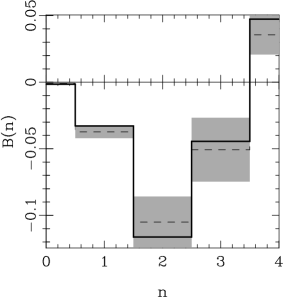
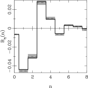
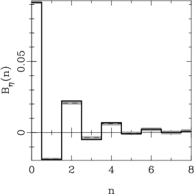
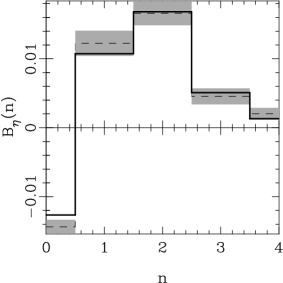
In Figs. 1–7 we present some numerical results that are obtained by a Monte-Carlo simulation of a quantum tomography experiment. The nonclassicality criterium is tested either on a Schrödinger-cat state $|\psi(\alpha)\rangle\propto(|\alpha\rangle+|-\alpha\rangle)$ or on a squeezed state $|\alpha,r\rangle\equiv D(\alpha)S(r)|0\rangle$, wherein $|\alpha\rangle$, $D(\alpha)$, and $S(r)$ denote a coherent state with amplitude $\alpha$, the displacement operator $D(\alpha)=e^{\alpha\hat{a}^{{\dagger}}-\bar{\alpha}\hat{a}}$, and the squeezing operator $S(r)=e^{r(\hat{a}^{{\dagger}2}-\hat{a}^{2})/2}$, respectively. Figs. 1–3 show tomographically-obtained values of $B(n)$, with the respective error bars superimposed, along with the theoretical values for a Schrödinger-cat state, for a phase-squeezed state ($r>0$), and for an amplitude-squeezed state ($r<0$), respectively. For the same set of states the results for $B_{\eta}(n)$ [cf. Eq. (7)] obtained by tomographic reconstruction of the noisy state are reported in Figs. 4–6. Let us compare the statistical errors that affect the two measurements, namely, those of $B(n)$ and $B_{\eta}(n)$ on the original and the noisy states, respectively. In the first case (Figs. 1–3) the error increases with $n$, whereas in the second (Figs. 4–6) it remains nearly constant, albeit with less marked oscillations in $B_{\eta}(n)$ than those in $B(n)$. Fig. 7 shows tomographically-obtained values of $B_{\eta}(n)$ for the phase-squeezed state (cf. Fig. 5), but for a lower quantum efficiency $\eta=0.4$. Notice that, in spite of the low quantum efficiency, the nonclassicality of such a state is still experimentally verifiable, as $B_{\eta}(0)<0$ by more than five standard deviations. In contrast, for coherent states one obtains small statistical fluctuations around zero for all $n$.

FIG. 3.: Same as in Fig. 2, but for an amplitude-squeezed state.

FIG. 4.: Tomographic measurement of $B_{\eta}(n)$ for a Schrödinger-cat state with $\bar{n}=5$, degraded by a quantum efficiency $\eta=0.8$. The number of simulated experimental data is $10^{7}$.

FIG. 5.: Tomographic measurement of $B_{\eta}(n)$ (dashed trace) with the respective error bars (superimposed in grey-shade) along with the theoretical values (solid trace) for a phase-squeezed state, which has $\bar{n}=5$ and $\bar{n}_{\rm sq}=\sinh^{2}r=3$ squeezing photons, and which has been degraded by a quantum efficiency $\eta=0.8$. For the reconstruction a sample of $10^{7}$ simulated experimental data have been used.

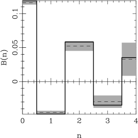
We remark that the simpler test of checking for antibunching or oscillations in the photon-number probability in the case of the phase-squeezed state considered here (Figs. 2, 5, and 7) would not reveal the nonclassical features of such a state.

FIG. 6.: Same as in Fig. 5, but for an amplitude-squeezed state.

FIG. 7.: Same as in Fig. 5, but here for a quantum efficiency of $\eta=0.4$, and a sample of $5\times 10^{7}$ simulated experimental data.

III TWO-MODE NONCLASSICALITY

Quantum homodyne tomography can also be employed to test the nonclassicality of two-mode states. For a two-mode state nonclassicality is defined in terms of nonpositivity of the following phase-averaged two-mode $P$-function [11]:

$$F(I_{1},I_{2},\phi)={1\over 2\pi}\int_{0}^{2\pi}d\phi_{1}\,P(I_{1}^{1/2}e^{i\phi_{1}},I_{2}^{1/2}e^{i(\phi_{1}+\phi)})\;.$$ (10)

In Ref. [11] it is also shown that a sufficient condition for nonclassicality is

$$C=\langle(\hat{n}_{1}-\hat{n}_{2})^{2}\rangle-(\langle\hat{n}_{1}-\hat{n}_{2}\rangle)^{2}-\langle\hat{n}_{1}+\hat{n}_{2}\rangle<0\;,$$ (11)

where $\hat{n}_{1}$ and $\hat{n}_{2}$ are the photon-number operators of the two modes.

A tomographic test of the inequality in Eq. (11) can be performed by averaging the kernel functions for the operators in the ensemble averages in Eq. (11) over the two-mode homodyne data. For the normal-ordered field operators one can use the Richter formula in Ref. [21], namely

$${\cal R}[a^{{\dagger}n}a^{m}](x,\phi)=e^{i(m-n)\phi}\,\frac{H_{n+m}(\sqrt{2\eta}x)}{\sqrt{(2\eta)^{n+m}}{n+m\choose n}}\;,$$ (12)

$H_{n}(x)$ denoting the Hermite polynomial and $\phi$ being the phase of the fiels with respect to the local oscillator of the homodyne detector. Again, as for the kernel function in Eq. (9), the value $\eta=1$ is used to reconstruct the ensemble averages of the noisy state $\hat{\rho}_{\eta}$. Notice that for $n=m$ Eq. (12) is independent on the phase $\phi$, and hence no phase knowledge is needed to reconstruct the ensemble averages in Eq. (11). As an example, we consider the twin-beam state at the output of a nondegenerate parametric amplifier

$$|\chi\rangle\equiv(1-|\lambda|^{2})\sum_{n=0}^{\infty}\lambda^{n}|n\rangle\otimes|n\rangle\;,$$ (13)

where $|n\rangle\otimes|n\rangle$ denotes the joint eigenvector of the number operators of the two modes with equal eigenvalue $n$, and the parameter $\lambda$ is related to the gain $G$ of the amplifier by the relation $|\lambda|^{2}=1-G^{-1}$. The theoretical value of $C$ for the state in Eq. (13) is $C=-2|\lambda|^{2}/(1-|\lambda|^{2})<0$. A tomographic reconstruction of the twin-beam state in Eq. (13) is particularly facilitated by the self-homodyning scheme, as shown in Ref. [22]. With regard to the effect of quantum efficiency $\eta<1$, the same argument still holds as for the single-mode case: one can evaluate $C_{\eta}$ for the twin-beam state that has been degraded by the effect of loss. In this case, the theoretical value of $C_{\eta}$ is simply rescaled to $C_{\eta}=-2\eta^{2}|\lambda|^{2}/(1-|\lambda|^{2})$.

FIG. 8.: Tomographic measurement of $C_{\eta}$ as defined in Eq. (11) and modified by the quantum efficiency for the twin-beam state in Eq. (13). The respective error bars are shown in the grey shade and $|\lambda|^{2}=0.5$ corresponding to an average of 2 total photons. The results are shown for various values of the quantum efficiency $\eta$ (in steps of 0.05) and for each value of $\eta$ the number of simulated data is $4\times 10^{5}$.

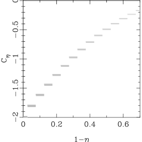
In Fig. 8 we report $C_{\eta}$ vs. $1-\eta$, $\eta$ ranging from 1 to 0.3 in steps of 0.05, for the twin-beam state in Eq. (13) with $|\lambda|^{2}=0.5$, corresponding to the total average photon number equal to 2. The values of $C_{\eta}$ result from a Monte-Carlo simulation of a homodyne tomography experiment with a sample of $4\times 10^{5}$ data, using the theoretical joint homodyne probability of the state $|\chi\rangle$

$$p_{\eta}(x_{1},x_{2},\phi_{1},\phi_{2})={2\exp\left[-{{(x_{1}+x_{2})^{2}}\over{d^{2}_{z}+4\Delta^{2}_{\eta}}}-{{(x_{1}-x_{2})^{2}}\over{d^{2}_{-z}+4\Delta^{2}_{\eta}}}\right]\over{\pi\sqrt{(d^{2}_{z}+4\Delta^{2}_{\eta})(d^{2}_{-z}+4\Delta^{2}_{\eta})}}}\;,$$ (14)

with

$$z=e^{-i(\phi_{1}+\phi_{2})}\Lambda\;,$$ (15)

$$d^{2}_{\pm z}={{|1\pm z|^{2}}\over{1-|z|^{2}}}\;,$$ (16)

$$\Delta^{2}_{\eta}=\frac{1-\eta}{4\eta}\;,$$ (17)

$\phi_{1}$ and $\phi_{2}$ denoting the phases of the two modes relative to the respective local oscillator. Notice that the nonclassicality test in terms of the noisy state gives values of $C_{\eta}$ that are increasingly near the classically positive region for decreasing quantum efficiency $\eta$. However, the statistical error remains constant and is sufficiently small to allow recognition of the nonclassicality of the twin-beam state in Eq. (13) up to $\eta=0.3$.

IV CONCLUSIONS

We have shown that quantum homodyne tomography allows one to perform nonclassicality tests for various single- and two-mode radiation states, even when the quantum efficiency of homodyne detection is rather low. The method involves reconstruction of the photon-number probability or of some suitable function of the number operators pertaining to the noisy state, namely, the state degraded by the less-than-unity quantum efficiency. The noisy-state reconstruction is affected by the statistical errors; however, they are sufficiently small that the nonclassicality of the state can be tested even for low values of $\eta$. For the cases considered in this paper, we have shown that the nonclassicality of the states can be proven (deviation from classicality by many error bars) with $10^{5}$–$10^{7}$ homodyne data. Moreover, since the knowledge of the phase of the local oscillator in the homodyne detector is not needed for the tomographic reconstruction, it can be left fluctuating in a real experiment. Hence, we conclude that the proposed nonclassicality test should be easy to perform experimentally.

REFERENCES

- [1] L. Mandel, Proc. Phys. Soc. 72, 1037 (1958).
- [2] C. K. Hong and L. Mandel, Phys. Rev. Lett. 54, 323 (1985); Phys. Rev. A 32, 974 (1985).
- [3] M. Hillery, Phys. Rev. A 36, 3796 (1987).
- [4] W. Schleich and J. A. Wheeler, Nature 326, 574 (1987).
- [5] Special issues on Squeezed states: J. Opt. Soc. Am. B 4, (H. J. Kimble and D. F. Walls, Eds.,1987); J. Mod. Opt. 34 (R. Loudon and P. L. Knight, Eds., 1987).
- [6] Squeezed and Non-classical Light, P. Tombesi and E. R. Pike, Eds., (Plenum Publishing, New York 1989).
- [7] G. S. Agarwal and K. Tara, Phys. Rev. A 46, 485 (1992).
- [8] C. T. Lee, Phys. Rev. A 44, R2775 (1991); Phys. Rev. A 52, 3374 (1995).
- [9] D. N. Klyshko, Phys. Usp. 37, 1097 (1994); Phys. Usp. 39, 573 (1996); Phys. Lett. A 213, 7 (1996).
- [10] Quantum Interferometry, F. De Martini et al., Eds. (VCH, Wenheim 1996).
- [11] Arvind, N. Mukunda, and R. Simon, J. Phys. A 31, 565 (1998).
- [12] K. Vogel and H. Risken, Phys. Rev. A 40, 2847 (1989).
- [13] G. M. D’Ariano, “Quantum estimation theory and optical detection,” in Quantum Optics and the Spectroscopy of Solids, T. Hakioǧlu and A. S. Shumovsky, Eds. (Kluwer, Dordrecht 1997) pp. 139-174.
- [14] G. M. D’Ariano, in “Quantum Communication, Computing, and Measurement”, ed. by O. Hirota, A. S. Holevo and C. M. Caves, Plenum Publishing (New York and London 1997), p. 253.
- [15] H. P. Yuen, Phys. Rev. A 13, 2226 (1976).
- [16] Y. Yamamoto and H. A. Haus, Rev. Mod. Phys. 58, 1001 (1986).
- [17] A. Bandilla, G. Drobný, and I. Jex, Phys. Rev. Lett. 75, 4019 (1995); Phys. Rev. A 53, 507 (1996).
- [18] J. Huang, Ph.D. thesis, Northwestern University, 1991 (unpublished).
- [19] G. M. D’Ariano, U. Leonhardt and H. Paul, Phys. Rev. A 52, R1801 (1995).
- [20] G. M. D’Ariano and C. Macchiavello, Phys. Rev. A 57, 3131 (1998).
- [21] Th. Richter, Phys. Rev. A 53, 1197 (1996).
- [22] G. M. D’Ariano, M. Vasilyev and P. Kumar, Phys. Rev. A 58, 636 (1998).