Quantum and Classical Noise in Practical Quantum Cryptography Systems based on polarization-entangled photons

Abstract

Quantum-cryptography key distribution (QCKD) experiments have been recently reported using polarization-entangled photons. However, in any practical realization, quantum systems suffer from either unwanted or induced interactions with the environment and the quantum measurement system, showing up as quantum and, ultimately, statistical noise. In this paper, we investigate how ideal polarization entanglement in spontaneous parametric downconversion (SPDC) suffers quantum noise in its practical implementation as a secure quantum system, yielding errors in the transmitted bit sequence. Because all SPDC-based QCKD schemes rely on the measurement of coincidence to assert the bit transmission between the two parties, we bundle up the overall quantum and statistical noise in an exhaustive model to calculate the accidental coincidences. This model predicts the quantum-bit error rate and the sifted key and allows comparisons between different security criteria of the hitherto proposed QCKD protocols, resulting in an objective assessment of performances and advantages of different systems.

I Introduction

Quantum Cryptography Key Distribution (QCKD) is at the moment the most advanced and challenging application of quantum information. QCKD offers the possibility that two remote parties, sender and receiver (conventionally called Alice and Bob), can exchange a secret random key, called sifted key (string of qubits), to implement a secure encryption/decryption algorithm based on a shared secret key, without the need that the two parties meet bennet&brassard ; ekert ; bb92 .

In practical QCKD, Alice and Bob use a quantum channel, along which sequences of signals are either sent or measured at random between different bases of orthogonal quantum states. Alice can play the role of either setting randomly the polarization basis of photons and sending them to Bob (faint laser pulses as photon source), or measuring photons randomly in any one of the selected bases (entangled photon source). Bob, randomly and independently from Alice, measures in one of the bases. The sifted key consists of the subset of measurements performed when Alice’s and Bob’s bases are in an agreed configuration according to the protocol used, obtaining at this point a deterministic outcome whose security relies on the laws of quantum physics, for they previously agreed upon the correspondence between counting a photon in a specific state and the bit values 0 or 1. In contrast, the security of conventional cryptography relies upon the unproven difficulty in factorizing large numbers into prime numbers by a conventional algorithm. We note that there is no guarantee that such an algorithm does not exist.

The underlying feature of QCKD, namely the reliance of the security of the distributed secret key on the laws of quantum physics bennet&brassard ; ekert ; bb92 , gives it an advantage over the public key cryptography. In other words, the uncertainty principle prohibits one from gaining information from a quantum channel without disturbing it. Basically, QCKD is founded on the principle that when a third party (Eve) performs a measurement on a qubit exchanged, she induces a perturbation, yielding errors in the bit sequence transmitted, revealing her presence. Any attempt by Eve to obtain information about the key leads to a nonzero error rate in the generated sifted key. Nevertheless this last claim must be somewhat softened because of practical realization of quantum channels brassard . Unfortunately, in practical systems, errors also happen because of experimental leakage, like losses in optics, detection, electronics and noise. Also, even when no eavesdropper is disturbing the bit exchange, there will be errors in the transmission and Alice’s and Bob’s strings will not coincide perfectly. Thus in practice there is no way to distinguish an eavesdropper attack from experimental imperfections, making it necessary to establish an upper bound on tolerable experimental imperfections in the realization of the quantum channels to implement an error correction procedure.

Following the first proposal by Bennett and Brassard bennet&brassard and later the Ekert protocol invoking entangled states ekert , various systems of QCKD have been implemented and tested by groups around the world. Recently some research groups ekertrarity ; sasha ; qk2 ; qk3 ; qk1 performed the first QCKD experiments based on polarization-entangled photon pairs, and Brassard et al. brassard proved theoretically that QCKD schemes based on spontaneous parametric down-conversion (SPDC) offer enhanced performance, mostly in terms of security, compared to QCKD based on weak coherent pulses.

Entangled photons, generated by SPDC in nonlinear crystals, have proved largely successful for quantum optical communication mandel ; rarity0 ; rarity ; rarity2 and quantum radiometry prl ; klyshko ; rarity4 ; peninserg ; kwiat ; migdall ; metrolo ; teichSaleh ; josaB ; madrideta . Furthermore, basic experimental tests of the foundation of quantum mechanics had been performed by exploiting the entanglement of this source rarity3 ; gisin1 ; zeil . However, quantum noise in a SPDC quantum state may significantly limit performance of the proposed quantum optical communication and information technologies.

In this paper we provide a general model for an a priori evaluation of some crucial parameters of a general QCKD scheme based on polarization entangled photons. We basically adopt the formalism of quantum operations NC00 to describe the dynamics of an open quantum system subject either to the interactions with the environment or to a quantum device performing a measurement on it. These unwanted or induced interactions show up as noise in quantum-information processing systems, degrading their ideal performance. Exploiting the quantum-operation formalism we present a model to quantify precisely both quantum and ultimately statistical noise in quantum-information experiments performed using an entangled photon source.

In Section II we consider quantum noise in a lossless measurement system where noise is due to the coupling between the polarization mode of the source with the polarizing beam splitter ports. In Section III we discuss the case of a lossy system, where noise is induced by detection deficiencies, such as losses of correlated photons from the presence of optical elements, non-ideal detectors, and electronic devices in either channel, and detector dark-counts.

The model concludes with the calculation of an overall probability of total coincidence counts, including an imperfect time-correlation measurement, ultimately yielding an estimate of accidental coincidences (Section IV).

This result is used in the calculation of the quantum bit error rate (QBER) for QCKD protocols, i.e., BB84 and the two variants of the Ekert’s protocol, based on CHSH and Wigner’s inequalities respectively (Section V). Previsions are also presented about the sifted and the corrected key, the quantum-bit error rate (QBER) before and after a standard error correction procedure. Finally we evaluate the performance of security criteria for Ekert’s protocols based on both the CHSH inequality and Wigner’s inequality (Section VI).

II Quantum noise in polarization selection of photon pairs

In this Section we consider a real either non-maximally entangled or partially mixed state resulting from both imperfect entangled state generation by SPDC and imperfect polarization state selection by real polarizing beam splitters (PBSs).

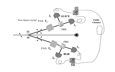
Figure 1: QCKD set-up: polarization-entangled photons generated by SPDC are directed to the two parties (Alice and Bob). The bit sequence of the key is obtained by means of polarization-sensitive synchronized measurements performed by Alice and Bob according to a specific QCKD protocol.

In Fig. 1 we depict the typical scheme for quantum cryptography key distribution as implemented using entangled photons generated by SPDC. Because of a nonlinear interaction in a $\chi^{(2)}$ crystal, some pump photons (angular frequency $\omega_{p}$) spontaneously split into a lower-frequency pair of photons, historically called signal and idler, perfectly correlated in all aspects of their state (direction, energy, polarization, under the constraints of conservation of energy and wavevector momentum, otherwise known as phase-matching). These entangled states show perfect correlation for polarization measured along orthogonal but arbitrary axes.

The QCKD performed by pure entangled states relies on the realization of two quantum correlated optical channels. These channels yield single-photon polarization states, such that whenever Alice performs a polarization measurement on a photon of the pair, automatically the other photon is projected in a defined polarization state, i.e., Alice plays the role of triggering Bob’s measurement. In actuality, the light field emerging from the output of the nonlinear crystal is a polarization-entangled multimode state. However, it can be described as a polarization entangled two-photon state in only two effective modes (one for channel $a$ and the other for channel $b$), as signal and idler pairs can be easily emitted non-collinearly with the pump by proper phase-matching rules opteng . This scheme eventually is exploited in quantum information applications by using one channel as the trigger or reference ($a$) and the other channel as the probe ($b$). According to Fig. 1, we denote Alice’s detector apparatus to be the trigger and Bob’s to be the probe. Alice and Bob detection apparatus consist of polarization-analyzer systems (PAS) for proper single-beam polarization rotation, polarizing beam splitters (PBS), photon detectors ($1_{a},\,2_{a},\,1_{b},\,2_{b}$), data storage systems (computers) and synchronization systems.

Let us consider in the following type II SPDC entangled states kwiat2 , where the output two-photon states are a quantum superposition of orthogonally polarized photons, i.e. the singlet state foot1 :

$$\left|\psi^{-}\right\rangle=\frac{1}{\sqrt{2}}\left(\left|H_{a}\right\rangle\left|V_{b}\right\rangle-\left|V_{a}\right\rangle\,\left|H_{b}\right\rangle\right).$$

Practically, pure entanglement may not be achieved because of imperfect source generation and because of incomplete entangled photon collection. According to Refs. scienceK ; berglund an uncompensated for coherence loss, induced in the state by the coupling between polarization and frequency modes because of a birefringent environment, may produce a partially mixed or non-maximally entangled state. Also the collection of the same number of entangled photons on both channels is unlikely, mostly due to the imperfect positioning of the detection systems along the true directions of entangled photons on the SPDC cones. Two complex variables, $\zeta$  ($\left|\zeta\right|\leqslant 1$) and $\epsilon$, characterize the imperfect compensation of dephasing and decoherence in the crystal and the misalignment in collecting entangled photons in the optical paths, respectevely. The net result is a non-maximally entangled, or partially mixed state, written as

$$\widehat{\rho}^{\psi} = \frac{1}{1+\left|\epsilon\right|^{2}}$$

$$\left[\begin{array}[]{c}\left|H_{a}\right\rangle\left|V_{b}\right\rangle\left\langle V_{b}\right|\left\langle H_{a}\right|+\left|\epsilon\right|^{2}\,\left|V_{a}\right\rangle\left|H_{b}\right\rangle\left\langle H_{b}\right|\left\langle V_{a}\right|+\\ -\epsilon\zeta\left|V_{a}\right\rangle\left|H_{b}\right\rangle\left\langle V_{b}\right|\left\langle H_{a}\right|-(\epsilon\zeta)^{\ast}\left|H_{a}\right\rangle\left|V_{b}\right\rangle\left\langle H_{b}\right|\left\langle V_{a}\right|\end{array}\right].$$

We analyze now the quantum noise introduced via an imperfect polarization state selection by the PBSs depicted in Fig. 1. Here, the entangled photons are detected accordingly to their polarizations by using imperfect polarizing beam splitters (PBSs) on both arms and perfect single-photon detectors. The PBSs project photons onto a polarization basis $\left\{\left|H_{a}\right\rangle\left|H_{b}\right\rangle,\left|V_{a}\right\rangle\left|V_{b}\right\rangle,\left|H_{a}\right\rangle\left|V_{b}\right\rangle,\left|V_{a}\right\rangle\left|H_{b}\right\rangle\right\},$ while the polarization analyzer systems (PASs) induce the transformations represented by the unitary operators $\widehat{T}_{z}$ in each arm ($z=a,b$), according to

$$\widehat{T}_{z}\left|H_{z}\right\rangle = c_{1}\left|H_{z}\right\rangle+c_{2}\left|V_{z}\right\rangle,$$

$$\widehat{T}_{z}\left|V_{z}\right\rangle = c_{2}\left|H_{z}\right\rangle-c_{1}\left|V_{z}\right\rangle.$$

In the case of ideal PBSs, channel $z$ transmits state $\left|H_{a}\right\rangle$ ($\left|H_{b}\right\rangle$) and reflects state $\left|V_{a}\right\rangle$ ($\left|V_{b}\right\rangle$), i.e., there is a perfect coupling between the output ports of the PBSs and the projections of the photon polarization state. In the approach so far adopted in the literature a perfect coupling is always assumed because the measurement process is considered as a projection on polarization states $\left|H_{a}\right\rangle,$ $\left|V_{a}\right\rangle$, $\left|H_{b}\right\rangle,$ $\left|V_{b}\right\rangle,$ thus assuming detectors $1_{a},\,1_{b},2_{a}\,,2_{b},$ are sensitive to polarization. Here we consider a further noise effect induced by the presence of real PBSs, where a small part of the photons projected onto $\left|V_{a}\right\rangle$ $(\left|V_{b}\right\rangle)$ are erroneously transmitted, and some photons projected in the state $\left|H_{a}\right\rangle$ $(\left|H_{b}\right\rangle)$ are erroneously reflected (generally less than 2 % and 5 %, respectively), as shown in Fig. 2. For this purpose, we extend the Hilbert space to describe these photon states as

$$\left|H_{z}\right\rangle\left|O1_{z}\right\rangle = t_{z}\left|H_{z}\right\rangle\left|I1_{z}\right\rangle+r_{z}\left|H_{z}\right\rangle\left|I2_{z}\right\rangle$$

$$\left|H_{z}\right\rangle\left|O2_{z}\right\rangle = t_{z}\left|H_{z}\right\rangle\left|I2_{z}\right\rangle+r_{z}\left|H_{z}\right\rangle\left|I1_{z}\right\rangle$$

$$\left|V_{z}\right\rangle\left|O1_{z}\right\rangle = r_{z}^{\perp}\left|V_{z}\right\rangle\left|I2_{z}\right\rangle+t_{z}^{\perp}\left|V_{z}\right\rangle\left|I1_{z}\right\rangle$$

$$\left|V_{z}\right\rangle\left|O2_{z}\right\rangle = r_{z}^{\perp}\left|V_{z}\right\rangle\left|I1_{z}\right\rangle+t_{z}^{\perp}\left|V_{z}\right\rangle\left|I2_{z}\right\rangle,$$ (2)

where $\left|Ox_{z}\right\rangle$ represents the photon crossing the output port of the PBS towards detector $x_{z}$ and $\left|Ix_{z}\right\rangle$ represents the photon crossing the input port of the PBS, with $x=1,2$. $\left|t_{z}^{\perp}\right|^{2}$ is the transmittance of photons in the $\left|V_{z}\right\rangle$ polarization state, and $\left|r_{z}^{\perp}\right|^{2}=1-$ $\left|t_{z}^{\perp}\right|^{2}$ is the corresponding reflectance, whose phase relation is $r_{z}^{\perp}/t_{z}^{\perp}=i\left|r_{z}^{\perp}\right|/\left|t_{z}^{\perp}\right|$. Analogously, $\left|t_{z}\right|^{2}$ and $\left|r_{z}\right|^{2}$ are the transmittance and reflectance of photons in the $\left|H_{z}\right\rangle$ state. So far, we have considered only lossless PBSs. The effect of photon losses due to all optical devices used in the channels are treated in Sections III and IV.

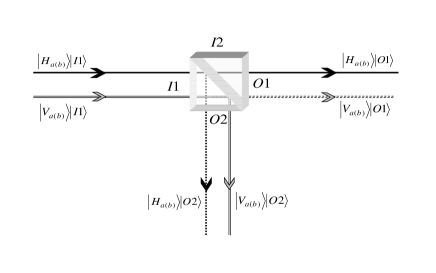
Figure 2: Real PBS: all photons projected in $\left|V_{a(b)}\right\rangle$ polarized state should be reflected, but some of these are wrongly transmitted. Moreover all photons projected in $\left|H_{a(b)}\right\rangle$ polarized state should be transmitted, but some of these are erroneously reflected.

We define the input density matrix for the PBS ports as

$$\widehat{\rho}^{\text{PBS}}=\left|I1_{a}\right\rangle\left|I1_{b}\right\rangle\left\langle I1_{b}\right|\left\langle I1_{a}\right|,$$

and the total input density matrix $\widehat{\rho}^{\text{in}}$ of the photon system as

$$\widehat{\rho}^{\text{in}}=\widehat{\rho}^{\psi}\otimes\widehat{\rho}^{\text{PBS}}.$$

The formalism of quantum operation is the most suitable to describe the evolution of a quantum system coupled with another quantum system or with the environment, as well as the evolution of a quantum system subject to measurement NC00 . In this context, we consider the set of non-trace-preserving quantum operations $\left\{\mathcal{E}_{x_{a}y_{b}}\right\}$ defined as

$$\mathcal{E}_{x_{a}y_{b}}\left(\widehat{\rho}^{\psi}\right)=\text{Tr}_{\text{PBS}}\left(\widehat{P}_{x_{a}y_{b}}\widehat{U}_{\psi\text{-PBS}}\widehat{S}_{\psi}\widehat{\rho}^{\text{in}}\widehat{S}_{\psi}^{\dagger}\widehat{U}_{\psi\text{-PBS}}^{\dagger}\widehat{P}_{x_{a}y_{b}}^{\dagger}\right),$$

describing the process of detection of the photon pair by the detectors $x_{a}$ and $y_{b}$ ($x,y=1,2$). In this expression, the unitary operator $\widehat{S}_{\psi}$ describes the action of the PASs and the unitary transformation $\widehat{U}_{\psi\text{-PBS}}$ describes the coupling between the photon pair polarization state and the PBS ports. The explicit form of $\widehat{U}_{\psi\text{-PBS}}$ is deduced by Eq.s (2), and calculations are reported in Appendix A. Because the operators $\widehat{T}_{a}$ and $\widehat{T}_{b}$ independently act on the corresponding subspaces $a$ and $b$ of the Hilbert space of polarization and induce linear transformation, they are ineffective on the Hilbert space of the PBS ports. Thus, $\widehat{\rho}^{\text{in}}$ is subject to a global transformation written as an unitary operator $\widehat{S}_{\psi}=\mathbf{1}^{\text{PBS}}\otimes\widehat{S}_{a,b},$ where  $\widehat{S}_{a,b}=\widehat{T}_{a}\otimes\widehat{T}_{b}.$

$\widehat{P}_{x_{a}y_{b}}=\left|Ox_{a}\right\rangle\left|Oy_{b}\right\rangle\left\langle Oy_{b}\right|\left\langle Ox_{a}\right|$ is the projector representing the detection process by the two detectors $x_{a}$ and $y_{b}.$ The probability of detection of the photon pair by the detectors $x_{a}$ and $y_{b}$ is

$$p(x_{a},y_{b}) = \text{Tr}_{\psi}\left[\mathcal{E}_{x_{a}y_{b}}\left(\widehat{\rho}^{\psi}\right)\right]=$$ (3)

$$= \text{Tr}\left(\widehat{P}_{x_{a}y_{b}}\widehat{U}_{\psi\text{-PBS}}\widehat{S}_{\psi}\widehat{\rho}^{\text{in}}\widehat{S}_{\psi}^{\dagger}\widehat{U}_{\psi\text{-PBS}}^{\dagger}\widehat{P}_{x_{a}y_{b}}^{\dagger}\right).$$

$\sum_{x_{a}y_{b}}\mathcal{E}_{x_{a}y_{b}}\left(\widehat{\rho}^{\psi}\right)$ is trace-preserving because the probabilities of the distinct outcomes sum to one, i.e., Tr${}_{\psi}\left[\sum_{x_{a}y_{b}}\mathcal{E}_{x_{a}y_{b}}\left(\widehat{\rho}^{\psi}\right)\right]=\sum_{x_{a}y_{b}}p(x_{a},y_{b})=1$ for all possible input $\widehat{\rho}^{\psi}.$

III Quantum and classical noise in photon counts

In the following we consider the noise contribution to the photon counts because of an imperfect collection of photons and a noisy and lossy detection system. For the experimental setup in Fig. 1, we calculate the total probability $p_{\text{tot},x_{z}}(n)$ of $n$ counts by any detector $x_{z}$ by separately calculating the probabilities of counts associated with correlated photons ($p_{sp,x_{z}}(n)$), with uncorrelated photons ($p_{u,x_{z}}(n)$), and with detector dark counts ($p_{d,x_{z}}(n)$).

To describe the counting process we adopt the formalism of quantum operations, where we consider a general density matrix representing photons on a channel $\nu$ in term of number of photons, i.e. $\left\{\left|n^{\nu}\right\rangle\right\},$ as

$$\widehat{\rho}^{\nu}=\sum_{n,m=0}^{\infty}\rho_{\,nm}^{\nu}\left|n^{\nu}\right\rangle\left\langle m^{\nu}\right|.$$ (4)

The evolution of the system $\widehat{\rho}^{\nu}$ is evaluated according to the formalism of quantum operations.

In this way, we define the set of non-trace-preserving quantum operations as $\left\{\mathcal{E}_{m}^{\mu}\right\}$ as

$$\mathcal{E}_{m}^{\mu}\left(\widehat{\rho}^{\nu}\right)=\text{Tr}_{\text{E}_{\mu}}\left(\widehat{P}_{m}^{\mu}\widehat{U}_{\text{Q}_{\nu}\text{-E}_{\mu}}\widehat{\rho}^{\nu}\otimes\left|e_{0}^{\mu}\right\rangle\left\langle e_{0}^{\mu}\right|\widehat{U}_{\text{Q}_{\nu}\text{-E}_{\mu}}^{\dagger}\widehat{P}_{m}^{\mu\;\dagger}\right),$$ (5)

which describes the detection of $m$ photons by the system $\mu$. In this expression the unitary operator $\widehat{U}_{\text{Q}_{\nu}\text{-E}_{\mu}}$ represents the interaction between the quantum system Q_ν of photons in the channel $\nu$ in the initial state $\widehat{\rho}^{\nu}$ and the lossy and noisy environment E_μ in the initial state $\left|e_{0}^{\mu}\right\rangle$. The action of $\widehat{U}_{\text{Q}_{\nu}\text{-E}_{\mu}}$ on the state “number of photons” is

$$\widehat{U}_{\text{Q}_{\nu}\text{-E}_{\mu}}\left|n^{\nu}\right\rangle\left|e_{0}^{\mu}\right\rangle=\sum_{m=0}^{n}d^{\mu}(m,n)\left|m^{\nu}\right\rangle\left|e_{m,n}^{\mu}\right\rangle$$ (6)

where $\left|d^{\mu}(m,n)\right|^{2}$ is the probability of measuring $m$ photons out of $n$ present in the channel $\nu$ because of losses. $\widehat{P}_{m}^{\mu}=\sum_{n=m}^{\infty}\left|e_{m,n}^{\mu}\right\rangle\left\langle e_{m,n}^{\mu}\right|$ are the measurement operators.

Thus, the probability of measuring $m$ counts by the detection system $\mu$ is

$$p_{\mu}(m)=\text{Tr}_{\text{Q}_{\nu}}\left[\mathcal{E}_{m}^{\mu}\left(\widehat{\rho}^{\nu}\right)\right]=\sum_{n=m}^{\infty}\rho_{\,nn}^{\nu}\left|d^{\mu}(m,n)\right|^{2}$$ (7)

where $\rho_{\,nn}^{\nu}$ is the probability of having $n$ photons on the channel $\nu$.

III.1 Single counts associated with correlated photons

In the following we concentrate primarily on the measurement of correlated photons by a lossy detector, $x_{z}$. We define the density matrix of the number of photon pairs, $\widehat{\rho}^{p}$, as

$$\widehat{\rho}^{p}=\sum_{n,m=0}^{\infty}\rho_{\,nm}^{p}\left|n^{p}\right\rangle\left\langle m^{p}\right|.$$ (8)

Analogous to Eq. (8), we write a density matrix of single photons of the pairs (sp) along channel $z$:

$$\widehat{\rho}^{sp,z}=\sum_{n,m=0}^{\infty}\rho_{\,nm}^{p}\left|n^{sp,z}\right\rangle\left\langle m^{sp,z}\right|.$$ (9)

The counting of correlated photons on channel $z$ by the detector $x_{z}$ is described by mapping $\widehat{\rho}^{sp,z}$ on the set of non-trace-preserving quantum operation $\left\{\mathcal{E}_{m}^{sp,x_{z}}\right\}$. The explicit form of $\mathcal{E}_{m}^{sp,x_{z}}\left(\widehat{\rho}^{sp,z}\right)$ is deduced by analogy to Eq. (5), by replacing the interaction unitary operator with $\widehat{U}_{\text{Q}_{sp,z}\text{-E}_{sp,x_{z}}}$ and the measurement operator with $\widehat{P}_{m}^{sp,x_{z}}$, given that Q_sp,z is the quantum system of single photons of the pair on the channel $z$ and E${}_{sp,x_{z}}$ is the lossy and noisy environment in the initial state $\left|e_{0}^{sp,x_{z}}\right\rangle$. The $\widehat{U}_{\text{Q}_{sp,z}\text{-E}_{sp,x_{z}}}$ action on the state $\left|n^{sp,z}\right\rangle$ is completely described by means of coefficients $d^{sp,x_{z}}(m,n)$ in complete analogy with Eq. (6), while we have $\widehat{P}_{m}^{sp,x_{z}}=\sum_{n=m}^{\infty}\left|e_{m,n}^{sp,x_{z}}\right\rangle\left\langle e_{m,n}^{sp,x_{z}}\right|$.

The probability of $m$ counts by the detector $x_{z}$ corresponding to correlated photons becomes

$$p_{sp,x_{z}}(m)=\sum_{n=m}^{\infty}\rho_{\,nn}^{p}\left|d^{sp,x_{z}}(m,n)\right|^{2}.$$ (10)

The probability of $n$ pairs is given by $\rho_{\,nn}^{p}=\left(\,\lambda_{p}t\right)^{n}\,\exp(-\lambda_{p}t)/n!,$ $t$ being the time of measurement and $\lambda_{p}$ the mean rate of photon pairs in the Alice and Bob channels teichSaleh ; capri ; Perina ; josab2 . The terms

$$\left|d^{sp,x_{a}}(m,n)\right|^{2} = \left(\begin{array}[]{c}n\\ m\end{array}\right)\left[\xi_{x_{a}}\sum_{y_{b}}p(x_{a},y_{b})\right]^{m}$$

$$\left[1-\xi_{x_{a}}\sum_{y_{b}}p(x_{a},y_{b})\right]^{n-m},$$

$$\left|d^{sp,y_{b}}(m,n)\right|^{2} = \left(\begin{array}[]{c}n\\ m\end{array}\right)\left[\xi_{y_{b}}\sum_{x_{a}}p(x_{a},y_{b})\right]^{m}$$

$$\left[1-\xi_{y_{b}}\sum_{x_{a}}p(x_{a},y_{b})\right]^{n-m}.$$

are the probabilities that only $m$ out of $n$ photons in the channel $a$ ($b$) are counted by the detector $x_{a}$ ($y_{b}$). Losses due to electronics ($\pi_{z}$), detection efficiencies ($\eta_{x_{z}}$), as well as optical losses ($\tau_{x_{z}}$) are summed up in the term $\xi_{x_{z}}=\pi_{z}\eta_{x_{z}}\tau_{x_{z}}$ josaB ; madrid ; while we refer to the Appendix B for the analysis of dead time in this context. The term $\tau_{x_{z}}$ incorporates all losses in the Alice and Bob optical path, such as from crystals, filters, lenses, PBSs, PASs and fibers. The terms $\sum_{x_{a}(y_{b})}p(x_{a},y_{b})$ are the probability that each photon of the pair may be counted randomly by any arbitrary detector (Eq. 3). Probability $p_{sp,x_{z}}(m)$ is derived according to Eq. (10), giving

$$p_{sp,x_{z}}(n)=\left(\lambda_{sp,x_{z}}t\right)^{n}\frac{\exp\left(-\lambda_{sp,x_{z}}t\right)}{n!},$$ (13)

with mean count rates given by

$$\lambda_{sp,x_{a}} = \xi_{x_{a}}\sum_{y_{b}}p(x_{a},y_{b})\lambda_{p},$$

$$\lambda_{sp,y_{b}} = \xi_{y_{b}}\sum_{x_{a}}p(x_{a},y_{b})\lambda_{p}.$$

III.2 Single counts associated with uncorrelated photons and dark counts

Here we consider counts from any detector $x_{z}$ from stray light, uncorrelated photons, and dark counts eventually contributing to noise in the distributed key. The density matrix associated with stray light and uncorrelated photons is

$$\widehat{\rho}^{u,x_{z}}=\sum_{n,m=0}^{\infty}\rho_{\,nm}^{u,x_{z}}\left|n^{u,x_{z}}\right\rangle\left\langle m^{u,x_{z}}\right|.$$

By pursuing the same formalism as before the detection of uncorrelated photons by the detector $x_{z}$ is described by means of the set of non-trace-preserving quantum operation $\left\{\mathcal{E}_{m}^{u,x_{z}}\right\}.$ The map $\mathcal{E}_{m}^{u,x_{z}}\left(\widehat{\rho}^{u,x_{z}}\right)$ follows in analogy with Eq. (5). The unitary operator $\widehat{U}_{\text{Q}_{u,x_{z}}\text{-E}_{u,x_{z}}}$ describes the interaction between the quantum system, Q${}_{u,x_{z}}$, of uncorrelated photons on the channel $x_{z}$ and the lossy environment, E${}_{u,x_{z}}$, in the initial state $\left|e_{0}^{u,x_{z}}\right\rangle$. The measurement operator is $\widehat{P}_{m}^{u,x_{z}}=\sum_{n=m}^{\infty}\left|e_{m,n}^{u,x_{z}}\right\rangle\left\langle e_{m,n}^{u,x_{z}}\right|.$ The action of $\widehat{U}_{\text{Q}_{u,x_{z}}\text{-E}_{u,x_{z}}}$ on the state $\left|n^{u,x_{z}}\right\rangle$ follows from Eq. (6) with the decomposition coefficients, $d^{u,x_{z}}(m,n)$.

Thus, the probability of measuring $m$ counts of uncorrelated photons by the detector $x_{z}$ is

$$p_{u,x_{z}}(m)=\sum_{n=m}^{\infty}\rho_{\,nn}^{u,x_{z}}\left|d^{u,x_{z}}(m,n)\right|^{2},$$ (14)

where $\rho_{\,nn}^{u,x_{z}}$ is the probability of $n$ uncorrelated photons in the channel $x_{z}$. According to Refs. teichSaleh ; capri ; Perina ; josab2 , we assume that we have $\rho_{\,nn}^{u,x_{z}}=\left(\lambda_{u,x_{z}}t\right)^{n}\exp\left(-\lambda_{u,x_{z}}t\right)/n!,$ where $\lambda_{u,x_{z}}$ is the mean rate of uncorrelated photons. The term

$$\left|d^{u,x_{z}}(m,n)\right|^{2}=\left(\begin{array}[]{c}n\\ m\end{array}\right)\left(\xi_{x_{z}}\right)^{m}\left(1-\xi_{x_{z}}\right)^{n-m}$$

is the probability of $m$ out of $n$ uncorrelated photons counted by the detector $x_{z}$.

The $p_{u,x_{z}}(n)$ derived accordingly from Eq. (14) is

$$p_{u,x_{z}}(n)=\left(\xi_{x_{z}}\lambda_{u,x_{z}}t\right)^{n}\frac{\exp\left(-\xi_{x_{z}}\lambda_{u,x_{z}}t\right)}{n!}.$$ (15)

The main source of noise in detectors is due to dark counts, whose distribution is regarded merely from a statistical point of view as the probability of $n$ dark counts

$$p_{d,x_{z}}(n)=\left(\,\lambda_{d,x_{z}}t\right)^{n}\,\frac{\exp(-\lambda_{d,x_{z}}t)}{n!},$$

with the mean dark-count rate being $\,\,\lambda_{d,x_{z}}$.

III.3 Total counts

As real counters cannot distinguish among counts due to correlated photons, counts due to uncorrelated photons, and dark counts, the total probability of measuring $k$ counts by detector $x_{z}$ is calculated according to teichSaleh ; capri ; josab2 ,

$$p_{\text{tot},x_{z}}(k)=\sum_{l,m,n=0}^{\infty}\delta_{k,l+m+n}\,p_{sp,x_{z}}(l)\,p_{u,x_{z}}(m)\,p_{d,x_{z}}(n),$$

giving

$$p_{\text{tot},x_{z}}(n)=\left(\,\lambda_{\text{tot},x_{z}}t\right)^{n}\frac{\exp(-\lambda_{\text{tot},x_{z}}t)}{n!},$$

where the mean rate of total counts measured by the detector $x_{z}$ is $\lambda_{\text{tot},x_{z}}=\lambda_{sp,x_{z}}+\xi_{x_{z}}\lambda_{u,x_{z}}+\lambda_{d,x_{z}}.$

IV Coincidence counts

We build up a model for the probability $p_{c,x_{a}y_{b}}(n)$ of measuring $n$ coincidences by a pair of detectors $x_{a}$ and $y_{b}$ in order to estimate crucial quantities of a typical QCKD experiment, such as the sifted key and the QBER before and after the error correction procedure, whenever different protocols are applied. We distinguish between the probability distribution of true coincidences ($p_{p,x_{a}y_{b}}(n),$ due to correlated photons) and the probability distribution of accidental coincidences ($p_{Acc,x_{a}y_{b}}(n)$, because of imperfections in the detection electronics).

We consider the density matrix in terms of counted pair states (Eq. (8)), and we describe its evolution exploiting the formalism of quantum operations as described in Section IV by defining another set of non-trace-preserving quantum operations $\left\{\mathcal{E}_{m}^{p,x_{a}y_{b}}\right\}.$

$\mathcal{E}_{m}^{p,x_{a}y_{b}}\left(\widehat{\rho}^{p}\right)$ describes the measurement of $m$ coincidences originated by the detection of the two photons of a pair by the detectors $x_{a}$, $y_{b}$. Its explicit expression is found from Eq. (5), except for the interaction between the quantum system Q_p of photon pairs in the initial state $\widehat{\rho}^{p}$ and the lossy and noisy environment E${}_{p,x_{a}y_{b}}$ in the initial state $\left|e_{0}^{p,x_{a}y_{b}}\right\rangle$ represented by the unitary operator $\widehat{U}_{\text{Q}_{p}\text{-E}_{p,x_{a}y_{b}}}$ and the measurement operator $\widehat{P}_{m}^{p,x_{a}y_{b}}=\sum_{n=m}^{\infty}\left|e_{m,n}^{p,x_{a}y_{b}}\right\rangle\left\langle e_{m,n}^{p,x_{a}y_{b}}\right|.$

The action of $\widehat{U}_{\text{Q}_{p}\text{-E}_{p,x_{a}y_{b}}}$ on the state “number of photon pairs” is

$$\widehat{U}_{\text{Q}_{p}\text{-E}_{p,x_{a}y_{b}}}\left|n^{p}\right\rangle\left|e_{0}^{p,x_{a}y_{b}}\right\rangle=\sum_{m=0}^{n}d^{p,x_{a}y_{b}}(m,n)\left|m^{p}\right\rangle\left|e_{m,n}^{p,x_{a}y_{b}}\right\rangle.$$

Thus, the probability of measuring $m$ true coincidences corresponding to photon pairs by the pair of detectors $x_{a},$ $y_{b}$ is

$$p_{p,x_{a}y_{b}}(m)=\sum_{n=m}^{\infty}\rho_{\,nn}^{p}\left|d^{p,x_{a}y_{b}}(m,n)\right|^{2}.$$ (16)

Realizing that a true coincidence may occur only if both photons of the pair are not lost, we emphasize that the terms $\left|d^{p,x_{a}y_{b}}(m,n)\right|^{2}$ are the probabilities that only $m$ pairs are detected as coincidences by the pair of detectors $x_{a}$, $y_{b}$ when $n$ photons are present in the Alice’s and Bob’s channels. It is straightforward to deduce the explicit form of $\left|d^{p,x_{a}y_{b}}(m,n)\right|^{2}$ as

$$\left|d^{p,x_{a}y_{b}}(m,n)\right|^{2} = \left(\begin{array}[]{c}n\\ m\end{array}\right)\left[\xi_{x_{a}}\xi_{y_{b}}p(x_{a},y_{b})\right]^{m}$$

$$\left[1-\xi_{x_{a}}\xi_{y_{b}}p(x_{a},y_{b})\right]^{n-m}.$$

Probability $p_{p,x_{a}y_{b}}(n)$ is derived according to Eq. (16), obtaining

$$p_{p,x_{a}y_{b}}(n)=\left(\lambda_{p,x_{a}y_{b}}t\right)^{n}\frac{\exp\left(-\lambda_{p,x_{a}y_{b}}t\right)}{n!}\,$$

where $\lambda_{p,x_{a}y_{b}}=\xi_{x_{a}}\xi_{y_{b}}p(x_{a},y_{b})\lambda_{p}$ is the mean rate of true coincidences seen by the pair of detectors $x_{a}$ and $y_{b}$.

IV.1 Accidental coincidences

The presence of the temporal coincidence window$\,w,$ during which coincidences are measured, modifies the mean total coincidence counts, thus forcing one to distinguish between true and accidental coincidence statistics. We assume that true coincidences occur in the middle of the coincidence temporal window. Then we deduce the probability distribution of accidental coincidences and finally the probability distribution of total coincidences, accounting for true and accidental coincidences, assuming $w<D_{z}$, where $D_{z}\$is the dead time in the $z$ channel according to Appendix B.

We regard $p_{\text{N},x_{z}}(n)$ as the probability distribution of photons counted by the detector $x_{z}$ that may contribute to accidental coincidences in the time interval $\Delta t$. By observing that the probability distributions $p_{\text{tot},x_{z}}(n)$ and $p_{p,x_{a}y_{b}}(n)$ are Poisson, it is simple to demonstrate that we have

$$p_{\text{N},x_{z}}(n)=\left(\lambda_{\text{N},x_{z}}\Delta t\right)^{n}\frac{\exp\left(-\lambda_{\text{N},x_{z}}\Delta t\right)}{n!},$$

where $\lambda_{\text{N},x_{a}}=\lambda_{\text{tot},x_{a}}-\lambda_{p,x_{a}y_{b}}$, and $\lambda_{\text{N},y_{b}}=\lambda_{\text{tot},y_{b}}-\lambda_{p,x_{a}y_{b}}$ are the mean count rates possibly contributing to accidental coincidences from the detectors $x_{a}$ and $y_{b}$, respectively.

Let us denote by $q_{y_{b}}$ the probability that at least one photon in $y_{b}$ is counted in the coincidence window $\Delta t=w$

$$q_{y_{b}}=\sum_{n=1}^{\infty}p_{\text{N},x_{z}}^{\Delta t=w}(n)=1-\exp\left(-\lambda_{\text{N},x_{z}}w\right),$$ (18)

because detectors $x_{a}$ are here considered as triggers.

The term in Eq. (18) is intended to account for the contribution of single detectors $y_{b}$. Because detectors $y_{b}$ are statistically independent, the probability that both detectors count a photon producing an accidental coincidence is $q_{1_{b}}\,q_{2_{b}}$. The final probability of accidental counts from detector $y_{b}$ is obtained by subtracting half the probability that both detectors in Bob’s channel count an accidental photon, in formula

$$q_{1_{b}}^{\ast} = q_{1_{b}}(1-\frac{1}{2}q_{2_{b}}),$$ (19)

$$q_{2_{b}}^{\ast} = q_{2_{b}}(1-\frac{1}{2}q_{1_{b}}).$$ (20)

According to teichSaleh ; capri ; Perina ; josab2 , we calculate the probability distribution of accidental coincidences in the time measurement $t$ by applying the discrete convolution between the Poisson distribution of “triggering” counts and the binomial distribution with parameter $q_{y_{b}}^{\ast},$

$$p_{Acc,x_{a}y_{b}}(m)=\sum_{n=m}^{\infty}p_{\text{N},x_{a}}(n)B_{y_{b}}\left(m,n\right)$$

with $B_{y_{b}}\left(m,n\right)=$

$\left(\begin{array}[]{c}n\\ m\end{array}\right)\left(q_{y_{b}}^{\ast}\right)^{m}\left(1-q_{y_{b}}^{\ast}\right)^{n-m},$ giving

$$p_{Acc,x_{a}y_{b}}(n)=\left(\lambda_{Acc,x_{a}y_{b}}t\right)^{n}\frac{\exp\left(-\lambda_{Acc,x_{a}y_{b}}t\right)}{n!}$$

with $\lambda_{Acc,x_{a}y_{b}}=q_{y_{b}}^{\ast}\lambda_{\text{N},x_{a}}.$

Lastly the probability distribution of total coincidence counts $p_{c,x_{a}y_{b}}(n)$ is obtained by

$$p_{c,x_{a}y_{b}}(k) = \sum_{m,n=0}^{\infty}\delta_{k,m+n}\,p_{p,x_{a}y_{b}}(m)\,p_{Acc,x_{a}y_{b}}(n)=$$

$$= \left(\,\lambda_{c,x_{a}y_{b}}t\right)^{n}\,\frac{\exp(-\lambda_{c,x_{a}y_{b}}t)}{n!},$$

where the mean rate of total coincidence measured by an arbitrary pair of $x_{a}$ and $y_{b}$ detectors is

$$\lambda_{c,x_{a}y_{b}}=\lambda_{p,x_{a}y_{b}}+\lambda_{Acc,x_{a}y_{b}}.$$ (21)

To characterize a particular QCKD procedure we embody the effect of the transformations $\widehat{T}_{a}$ and $\widehat{T}_{b}$ on photon polarization by the rotation matrices

$$\widehat{T}_{z}=\left(\begin{array}[]{cc}\cos\theta_{z}&\sin\theta_{z}\\ \sin\theta_{z}&-\cos\theta_{z}\end{array}\right).$$ (22)

We rewrite Eq. (21) in terms of the rotation angles $\theta_{a},\theta_{b},$ induced by transformations $\widehat{T}_{a}$ and $\widehat{T}_{b}$ on the polarization state of photons, by replacing $p(x_{a},y_{b})$ with $p_{\theta_{a},\theta_{b}}(x_{a},y_{b}),$ whose complete expression is in Appendix A. More specifically, the calculated mean coincident counts are made explicit in terms of angular settings $\theta_{a}$ and $\theta_{b}$ as $\lambda_{c,x_{a}y_{b}}(\theta_{a},\theta_{b})t.$

V evaluation of QBER

To characterize a particular QCKD procedure and to assess its advantages, we evaluate particular quantities such as the QBER and the sifted key for different types of QCKD protocols so far experimentally implemented, i.e. BB84 protocol and Ekert’s protocols based on CHSH and Wigner’s inequalities, respectively.

The QBER is a parameter for describing the signal quality in the transmission of the sifted key, defined as the relative frequency of errors induced by accidental coincidences, i.e. the number of errors divided by the total size of the cryptographic sifted key ($K$) josab2 .

In other words, the QBER is given by total coincidence provided by those detectors “wrongly” firing in coincidence according to the chosen protocol. In fact the protocol establishes which pair of detectors should fire to contribute to the key.

V.1 BB84 protocol

Here we examine the BB84 protocol variant proposed for entangled states in ref. bb92 . Recall that Alice and Bob measure photons randomly and independently between two bases of orthogonal quantum states. One basis corresponds to horizontal and vertical linear polarization ($\oplus$), while the other to linear polarizations rotated by 45^∘ ($\otimes$). Only half of the photon pairs can contribute to the sifted key, as only the subset of measurements performed with the two analyzers in the same basis contributes.

The sifted key is given by

$$K_{\text{BB84}}(\theta_{a}) = f_{basis}f_{setting}$$ (26)

$$\sum_{x_{a}y_{b}}\left[\begin{array}[]{c}\lambda_{c,x_{a}y_{b}}(\theta_{a},\theta_{a})+\\ \lambda_{c,x_{a}y_{b}}(\theta_{a}+\pi/4,\theta_{a}+\pi/4)\end{array}\right]t,$$

where $f_{basis}=1/2$ is the probability to measure in the right basis ($(\theta_{a},\theta_{a})$ and $(\theta_{a}+\pi/4,\theta_{a}+\pi/4)$), while $f_{setting}=1/2$ is the probability to measure in a particular analyzer setting ($(\theta_{a},\theta_{a})$ or $(\theta_{a}+\pi/4,\theta_{a}+\pi/4)$).

All detectors contribute to the sifted key $K$, but only coincidences between $1_{a}2_{b}$ and $2_{a}1_{b}$ correspond to the expected anticorrelation when measurements are performed in the same basis ($\theta_{a}=\theta_{b}$), while QBER contributions come from the coincidences between detectors $1_{a}1_{b}$ and $2_{a}2_{b}$ (as it is clear from Eq.s (32) in Appendix A). Therefore the QBER${}_{\text{BB84}}$ explicit formula is

$$\text{QBER}_{\text{BB84}}(\theta_{a})\text{=}\frac{\sum_{x=1,2}\left[\begin{array}[]{c}\lambda_{c,x_{a}x_{b}}(\theta_{a},\theta_{a})+\\ \lambda_{c,x_{a}x_{b}}(\theta_{a}+\pi/4,\theta_{a}+\pi/4)\end{array}\right]t}{4K_{\text{BB84}}(\theta_{a})}.$$ (27)

To test the behavior of QBER, we simulate a realistic experiment with parameters $\eta_{x_{a}}=\eta_{y_{b}}=0.5$ (quantum efficiency of the four detectors), $\tau_{x_{a}}=\tau_{y_{b}}=0.1$ (transmittance of the four channels), $\lambda_{d,x_{a}}=\lambda_{d,y_{b}}=50$ s^-1 (dark count rate of the four detectors), $D_{a}=D_{b}=100$ ns (total dead time of the Alice’s and Bob’s detection systems), $\theta_{a}=0$ and $w=4$ ns. The entanglement parameters are $\epsilon=0.95$ and $\zeta=1,$ the correlation level in the Alice channel is $\alpha_{a}=0.25$ ($\alpha_{a}=\lambda_{p}/(\lambda_{p}+\sum_{x_{a}}\lambda_{u,x_{a}})$), and the correlated photon rate is $\lambda_{p}=700\,$KHz.

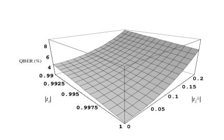
Figure 3: QBER for the BB84 protocol versus the PBS’s coefficients $\left|t_{z}\right|$ and $\left|t_{z}^{\perp}\right|.$

In Fig. 3 we show the dependence of QBER versus the optical properties of real PBS, i.e. the transmittance $\left|t_{z}\right|$ and $\left|t_{z}^{\perp}\right|$ ($z=a,b$) for the states $\left|H_{z}\right\rangle$ and $\left|V_{z}\right\rangle$ respectively. Results show how strongly the QBER can be affected by the optical properties of PBSs, whose influence has been neglected so far.

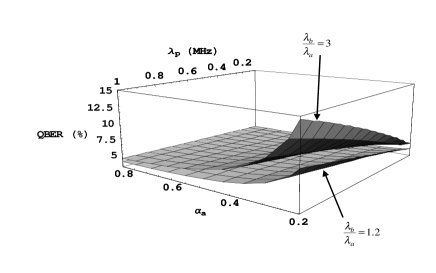
Figure 4: QBER for the BB84 protocol versus the correlation level in the Alice channel $\alpha_{a}=\lambda_{p}/(\lambda_{p}+\sum_{x_{a}}\lambda_{u,x_{a}})$ and the correlated photon rate $\lambda_{p}$ for two noise levels in the channels ($\lambda_{b}/\lambda_{a}=1.2$ and $3$, where $\lambda_{a}=\lambda_{p}+\sum_{x_{a}}\lambda_{u,x_{a}}$ and $\lambda_{b}=\lambda_{p}+\sum_{y_{b}}\lambda_{u,y_{b}}$).

In Fig. 4 the behavior of the QBER is presented versus the level of correlation, $\alpha_{a}$, in the Alice channel and the rate, $\lambda_{p}$, of the correlated photon pairs for two different noise levels, i.e., the ratio between the mean rate of photons in the two channels. Far from ideal conditions, the presence of uncorrelated events in the two channels induces a non-linear increase of the QBER. The other parameters are set as in Fig. 3 for realistic PBSs parameters, $\left|t_{z}\right|^{2}=0.99$ and $\left|t_{z}^{\perp}\right|^{2}=0.025$.

V.2 Ekert’s protocol

Ekert’s protocol has the peculiarity of relying on the completeness of quantum mechanics for security. Therefore, the possible combined choices between Alice and Bob for analyzer settings split into three groups: the first for key distribution, the second containing the security proof, and the third garnering the discarded measurements.

Here we consider two possible variants of Ekert’s protocol: the variant based on the Clauser-Horne-Shimony-Holt inequality (CHSH), similar to the one proposed in Ref. qk3 , and the variant based on Wigner’s inequality qk2 .

V.2.1 Ekert’s protocol based on CHSH inequalities

To increase the number of measurements devoted to the key distribution we consider the case where Alice and Bob measure randomly among four analyzer settings and use the CHSH inequality to test eavesdropping. In this scheme, Alice’s choices for the analyzer settings are $\theta_{a}=(\theta_{a},\theta_{a}+\pi/8,\theta_{a}+\pi/4,\theta_{a}+3\pi/8)$ and Bob’s are $\theta_{b}=(\theta_{a}+\pi/8,\theta_{a}+\pi/4,\theta_{a}+3\,\pi/8,\theta_{a}+\pi/2)$.

The key distribution is performed when Alice and Bob’s settings are the same or orthogonal, so that the sifted key is

$$K_{\text{CHSH}}(\theta_{a}) = f_{setting}$$

$$\sum_{x_{a}y_{b}}\left[\begin{array}[]{c}\lambda_{c,x_{a}y_{b}}(\theta_{a},\theta_{a}+\pi/2)+\\ \lambda_{c,x_{a}y_{b}}(\theta_{a}+\pi/8,\theta_{a}+\pi/8)+\\ \lambda_{c,x_{a}y_{b}}(\theta_{a}+\pi/4,\theta_{a}+\pi/4)+\\ \lambda_{c,x_{a}y_{b}}(\theta_{a}+3\pi/8,\theta_{a}+3\pi/8)\end{array}\right]t,$$

where ($(\theta_{a},\theta_{a}+\pi/2),\,(\theta_{a}+\pi/8,\theta_{a}+\pi/8),\,(\theta_{a}+\pi/4,\theta_{a}+\pi/4),(\theta_{a}+3\pi/8,\theta_{a}+3\pi/8))$ are angular settings generating the key and $f_{setting}=1/16.$

In a maximally entangled state configuration, the detectors contributing to the key should be $1_{a}1_{b}$ and $2_{a}2_{b}$ for the orthogonal analyzer settings and $1_{a}2_{b}$ and $2_{a}1_{b}$ for the parallel settings.  Thus the QBER is calculated according to

$$\text{QBER}_{\text{CHSH}}(\theta_{a})\text{=}\frac{1}{4K_{\text{CHSH}}(\theta_{a})}\left\{\sum_{x_{a},y_{b}(x\neq y)}\lambda_{c,x_{a}y_{b}}(\theta_{a},\theta_{a}+\pi/2)t+\sum_{x_{a},y_{b}(x=y)}\left[\begin{array}[]{c}\lambda_{c,x_{a}y_{b}}(\theta_{a}+\pi/8,\theta_{a}+\pi/8)+\\ \lambda_{c,x_{a}y_{b}}(\theta_{a}+\pi/4,\theta_{a}+\pi/4)+\\ \lambda_{c,x_{a}y_{b}}(\theta_{a}+3\pi/8,\theta_{a}+3\pi/8)\end{array}\right]t\right\},$$

where the intuitive notation $\sum_{x_{a},y_{b}(x\neq y)}$ indicates the sum over $1_{a}2_{b}$ and $2_{a}1_{b}$ detectors and $\sum_{x_{a},y_{b}(x=y)}$ indicates the sum over $1_{a}1_{b}$ and $2_{a}2_{b}.$

V.2.2 Ekert’s protocol based on Wigner’s inequality

As in Ref. qk2 , we consider the case of the Ekert’s variant where the security of the quantum channels follows from Wigner’s inequality. In this case, Alice and Bob measure randomly among four analyzers settings whose choices are $\theta_{a}=(\theta_{a}-\pi/6,\theta_{a})$ for Alice and $\theta_{b}=(\theta_{a},\theta_{a}+\pi/6)$ for Bob. The key distribution is performed when Alice’s and Bob’s settings are the same so that the sifted key is

$$K_{\text{WI}}(\theta_{a})=f_{setting}\sum_{x_{a}y_{b}}\lambda_{c,x_{a}y_{b}}(\theta_{a},\theta_{a})t,$$

with $f_{setting}=1/4.$

The QBER is calculated according to

$$\text{QBER}_{\text{WI}}(\theta_{a})\text{=}f_{setting}\frac{\left[\lambda_{c,1_{a}1_{b}}(\theta_{a},\theta_{a})+\lambda_{c,2_{a}2_{b}}(\theta_{a},\theta_{a})\right]t}{K_{\text{WI}}(\theta_{a})},$$

by taking the detectors contributing to the wrong bits as $1_{a}1_{b}$ and $2_{a}2_{b}.$

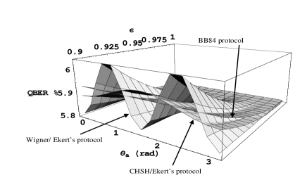
Figure 5: QBER in the case of CHSH and Wigner’s inequality based Ekert’s protocols together with BB84 protocol versus the angular analyzers settings $\theta_{a}$ and the entanglement parameter $\epsilon$. The parameters settings are $\lambda_{a}=2.8$ $10^{6}$ s${}^{-1},$ $\alpha_{a}=0.25,$ $\lambda_{b}/\lambda_{a}=1.2,$ $\eta_{x_{a}}=\eta_{y_{b}}=0.5,$ $\tau_{x_{a}}=\tau_{y_{b}}=0.1,$ $\lambda_{d,x_{a}}=\lambda_{d,y_{b}}=50$ s^-1, $D_{a}=D_{b}=100$ ns, $w=4$ ns and $\zeta=1$, taken from typical and experimental realistic values so far implemented. PBSs are considered real with $\left|t_{z}\right|^{2}=0.99$ and $\left|t_{z}^{\perp}\right|^{2}=0.025$ ($z=a,b$).

In Fig. 5 we present a comparison of QBER levels for the BB84 protocol and the Ekert protocols considering both CHSH and Wigner’s inequality versus the analyzers angular setting $\theta_{a}$ and the entanglement parameter $\epsilon$. Experimental conditions are the same (low noise) as for Figs. 3 and 4. Results highlight that the QBER is sensitive to the angle $\theta_{a}$ when the ideal entanglement is not achieved for both variants of Ekert’s protocols. In the Wigner’s case, the sensitivity is so remarkable that this protocol has to be considered less robust than BB84 and the CHSH based Ekert’s protocol.

VI Security and error correction

The security of the BB84 variant protocol is based on a public comparison between Alice and  Bob’s measurements on a sufficiently large random subset of the sifted key, e.g. more than half is recommended in bb92 .

The security proof for the CHSH-inequality-based Ekert’s protocol is evaluated with the specific choices of settings by the CHSH inequality,

$$S(\theta_{a}) = E(\theta_{a},\theta_{a}+\pi/8)-E(\theta_{a},\theta_{a}+3\pi/8)+$$

$$E(\theta_{a}+\pi/4,\theta_{a}+\pi/8)+E(\theta_{a}+\pi/4,\theta_{a}+3\pi/8),$$

$$S^{\prime}(\theta_{a}) = E(\theta_{a}+\pi/8,\theta_{a}+\pi/4)-E(\theta_{a}+\pi/8,\theta_{a}+\pi/2)+$$

$$E(\theta_{a}+3\pi/8,\theta_{a}+\pi/4)+E(\theta_{a}+3\pi/8,\theta_{a}+\pi/2),$$

where we have

$$E(\theta_{a},\theta_{b}) = M_{1_{a}1_{b}}(\theta_{a},\theta_{b})-M_{1_{a}2_{b}}(\theta_{a},\theta_{b})+$$

$$M_{2_{a}2_{b}}(\theta_{a},\theta_{b})-M_{2_{a}1_{b}}(\theta_{a},\theta_{b}).$$

Here

$$M_{x_{a}y_{b}}(\theta_{a},\theta_{b})=\frac{\lambda_{c,x_{a}y_{b}}(\theta_{a},\theta_{b})}{\sum_{x_{a}y_{b}}\lambda_{c,x_{a}y_{b}}(\theta_{a},\theta_{b})}$$

is the normalized coincidence rate as a function of the analyzer settings and detector choices. The terms $M_{x_{a}y_{b}}(\theta_{a},\theta_{b})$ are commonly stored when experiments are performed.

For maximally entangled states we have $\left|S_{\text{ql}}\right|=\left|S_{\text{ql}}^{\prime}\right|=2\sqrt{2}$, while for any realistic local theory we have $\left|S,S^{\prime}\right|\leq 2.$ It is expected that the presence of an eavesdropper will reduce the observed value of $\left|S,S^{\prime}\right|,$ giving $\left|S_{\text{eve}},S_{\text{eve}}^{\prime}\right|\leq\sqrt{2},$ when the eavesdropper measures photons over either one or both (total eavesdropping) of Alice’s and Bob’s channels ekert .

In the case of Wigner’s-inequality-based Ekert’s protocol, the Wigner’s inequality result has

$$W(\theta_{a}) = M_{1_{a}1_{b}}(\theta_{a}-\pi/6,\theta_{a})+M_{1_{a}1_{b}}(\theta_{a},\theta_{a}+\pi/6)+$$

$$-M_{1_{a}1_{b}}(\theta_{a}-\pi/6,\theta_{a}+\pi/6),$$

giving for the maximally entangled states, $W_{\text{ql}}=-1/8$ and $W\geq 0$ for any local realistic theory. As for the CHSH inequality, it can be proved that the limit becomes $W_{\text{eve}}\geq 1/16$ for Eve detecting only one photon of the pair, while in the case of total eavesdropping there is no boundary condition pc .

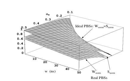
Figure 6: The CHSH and Wigner’s inequalities parameters S${}_{\text{norm}}$ and W${}_{\text{norm}}$ versus the coincidence window $w$ and the correlation level in the Alice channel $\alpha_{a}$. In the case of maximally entangled states we have W${}_{\text{norm}}=$S${}_{\text{norm}}=$1, while the lower cut is defined by the eavesdropping limit W${}_{\text{norm}}\leq 0$ and S${}_{\text{norm}}\leq 0$ . The choice of parameter values are the same of Fig. 4 except for $\theta_{a}=0$ and $\epsilon=0.95$. The lower two surfaces represented correspond to W${}_{\text{norm}}$ and S${}_{\text{norm}}$ in the case of real PBSs, with parameters $\left|t_{z}\right|^{2}=0.98$ and $\left|t_{z}^{\perp}\right|^{2}=0.05.$ The higher surface represents S${}_{\text{norm}}$=W${}_{\text{norm}}$ in the case of ideal PBSs.

In Fig. 6 we compare the behaviors of the CHSH and Wigner’s inequality parameters, $S_{\text{norm}}$ =$\left(\left|S\right|-\left|S_{\text{eve}}\right|\right)/\left(\left|S_{\text{ql}}\right|-\left|S_{\text{eve}}\right|\right)$ and $W_{\text{norm}}=\left(W-W_{\text{eve}}\right)/\left(W_{\text{ql}}-W_{\text{eve}}\right),$ versus the coincidence window $w$ and the correlation level in Alice’s channel, $\alpha_{a}.$ The lower surfaces represent the case of real PBSs, where $W_{\text{norm}}<$ $S_{\text{norm}}$, while the upper surface corresponds to  ideal PBSs, where $W_{\text{norm}}=$ $S_{\text{norm}}$. We observe that, given the same noise level in the system and real PBSs, Wigner’s parameter reaches the eavesdropping limit faster than the CHSH one does, revealing the intrinsic weakness of Wigner’s test against experimental parameters.

Furthermore, the Wigner’s security test guarantees against eavesdropping strategies only for the detection of one photon of the pair, while the CHSH security is independent on the adopted strategy (see refs. ekert ; pc ).

A satisfactory protocol must be able to recover from noise as well as from partial leakage, allowing Alice and Bob to reconcile the two strings of bits measured and distill from the sifted key a corrected key. A strong need for the application of any error-correction method is an a priori knowledge of the QBER, which provides information regarding how many times the error-correction procedure must be applied to reduce the QBER to a certain agreed level, commonly 1 %. Here, we show an example of error correction on an a priori evaluated QBER according to a common approach reported in Ref. qk2 , to show that our model allows for prediction of the corrected key length.

In general, Alice and Bob cannot distinguish between errors caused either by an eavesdropper or by the environment. Thus, they must assume that all errors are due to an eavesdropper and evaluate the leaked information from the QBER. Also, even though by the error-correction procedure one can disregard incorrect bits by simply dropping them off in building the distilled key, the residual knowledge of an eavesdropper may still not be faithfully quantified by the reduced QBER obtained after the correction. The effects of Eve’s strategy is in fact equivalent to quantum noise yielding eventually accidental coincidences, these last contributing to both incorrect and correct bits transmitted, as it is clear from Eqs. (26, 27). Hence the error-correction procedure is not sufficient to cancel a potential Eve’s knowledge of part of the key due to accidental coincidence.

To prove this last assertion we introduce the quantum accidental bit rate (QABR), a quantity related to accidental coincidences and, in this sense, analogous to the QBER. However, the error-correction procedure cannot reduce the QABR at the QBER level. As an example, we give the QABR in the case of Ekert’s protocol based on Wigner’s inequality,

$$\text{QABR}_{\text{WI}}(\theta_{a})\text{=}f_{setting}\frac{\sum_{x_{a}y_{b}}\lambda_{Acc,x_{a}y_{b}}(\theta_{a},\theta_{a})t}{K_{\text{WI}}(\theta_{a})}.$$

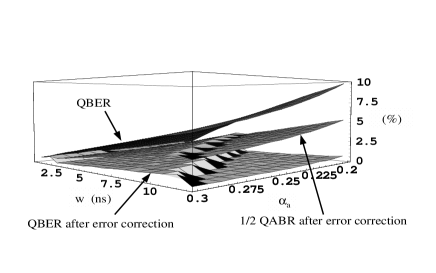
Figure 7: QBER in the case of BB84 protocol versus the coincidence window $w$ and the correlation parameter in the Alice channel $\alpha_{a}$: the sawtooth shape is due to the application of the error correction procedure. The parameters are set as in Figure 6 except that, in this case, ideal PBSs are considered.

Figure 7 shows the QBER with and without the application of the error-correction procedure together with the 1/2 QABR vs the coincidence window and the correlation parameter in Alice’s channel. The error-correction procedure is very ineffective at reducing the QABR and consequently the possible effect of Eve’s knowledge on the corrected key.

VII Conclusions

This paper is concerned with an a priori evaluation of QCKD crucial parameters when entangled photons produced by SPDC are exploited. The basic experimental feature consists in the detection of coincident photons. Toward this aim, we developed a statistical model to calculate the probability of accidental coincidences contributing to errors in the sifted key, not completely accounted for by simple experimental means.

We investigated the noise contribution due to imperfect source generation and selection, imperfect polarizing beam splitters performing polarization states analysis, and noisy and lossy measurement system for photon-number detection. We emphasized some basic system imperfections such as uncorrelated photons collection, detection system deficiencies, detection system noise due to detector dark counts, and electronic system imperfections associated with non-ideal-time-correlation measurements.

We discussed how this model can be adopted for the evaluation of the QBER and the sifted key for different well-known protocols, i.e., BB84 and Ekert’s protocols based on both CHSH and Wigner’s inequality, and compared them to expected results.

Given that this model predicts precisely the QBER and the sifted key, it ultimately guarantees a method to compare different security criteria of the hitherto proposed QCKD protocols and provides an objective assessment of performances and advantages of different systems. Thus, it yields a method for an a priori evaluation of the tolerable experimental imperfections in a practically implemented quantum system to establish the degree of security and competitiveness of QCKD systems.

Finally, we used the model in a standard error-correction procedure, observing that this does not completely cancel the possible residual eavesdropping knowledge on the corrected key. We emphasize that this model yields also the degree of security of the corrected key, if a precise modelling of system imperfections is provided.

Acknowledgment. This work was developed in collaboration with Elsag S.p.A., Genova (Italy), within a project entitled “Quantum Cryptographic Key Distribution” co-funded by the Italian Ministry of Education, University and Research (MIUR) - grant n. 67679/ L. 488. In addition Stefania Castelletto acknowledges the partial support of the DARPA QuIST program.

Appendix A Interaction matrix $\widehat{U}_{\psi\text{-PBS}}$

We explicitly calculate the unitary transformation $\widehat{U}_{\psi\text{-PBS}}$ according to Eq.s (2) obtaining a 16$\times$16 matrix

$$\widehat{U}_{\psi\text{-PBS}}=\left(\begin{array}[]{cccc}U_{1}&U_{2}&U_{3}&U_{4}\\ U_{2}&U_{1}&U_{4}&U_{3}\\ U_{3}&U_{4}&U_{1}&U_{2}\\ U_{4}&U_{3}&U_{2}&U_{1}\end{array}\right),$$

where we indicate

$$U_{1} = \left[\begin{array}[]{cccc}{\cal T}_{a}{\cal T}_{b}&0&0&0\\ 0&{\cal T}_{a}{\cal T}_{b}^{\perp}&0&0\\ 0&0&{\cal T}_{a}^{\perp}{\cal T}_{b}&0\\ 0&0&0&{\cal T}_{a}^{\perp}{\cal T}_{b}^{\perp}\end{array}\right];\;\;\;\;\;U_{2}=\left[\begin{array}[]{cccc}{\cal T}_{a}{\cal R}_{b}&0&0&0\\ 0&{\cal T}_{a}{\cal R}_{b}^{\perp}&0&0\\ 0&0&{\cal T}_{a}^{\perp}{\cal R}_{b}&0\\ 0&0&0&{\cal T}_{a}^{\perp}{\cal R}_{b}^{\perp}\end{array}\right]$$

$$U_{3} = \left[\begin{array}[]{cccc}{\cal R}_{a}{\cal T}_{b}&0&0&0\\ 0&{\cal R}_{a}{\cal T}_{b}^{\perp}&0&0\\ 0&0&{\cal R}_{a}^{\perp}{\cal T}_{b}&0\\ 0&0&0&{\cal R}_{a}^{\perp}{\cal T}_{b}^{\perp}\end{array}\right];\;\;\;\;\;\;\;\;U_{4}=\left[\begin{array}[]{cccc}{\cal R}_{a}{\cal R}_{b}&0&0&0\\ 0&{\cal R}_{a}{\cal R}_{b}^{\perp}&0&0\\ 0&0&{\cal R}_{a}^{\perp}{\cal R}_{b}&0\\ 0&0&0&{\cal R}_{a}^{\perp}{\cal R}_{b}^{\perp}\end{array}\right]$$

and $\mathcal{T}_{z}=t_{z}/(t_{z}^{2}-r_{z}^{2})$, $\mathcal{R}_{z}=r_{z}/(t_{z}^{2}-r_{z}^{2})$ $(z=a,b),$ analogously for $\mathcal{T}_{z}^{\perp}$ and $\mathcal{R}_{z}^{\perp}.$

According to Eq.s (3) and (22) we obtain for $p_{\theta_{a},\theta_{b}}(x_{a},y_{b})$ the following:

$$p_{\theta_{a},\theta_{b}}(1_{a},1_{b})=\frac{1}{1+\left|\epsilon\right|^{2}}\left\{\begin{array}[]{c}\cos^{2}(\theta_{b})\left[\begin{array}[]{c}\cos^{2}(\theta_{a})\left(\left|\mathcal{T}_{a}\mathcal{T}_{b}^{\perp}\right|^{2}+\left|\mathcal{T}_{a}^{\perp}\mathcal{T}_{b}\epsilon\right|^{2}\right)+\sin^{2}(\theta_{a})\left(\left|\mathcal{T}_{a}^{\perp}\mathcal{T}_{b}^{\perp}\right|^{2}+\left|\mathcal{T}_{a}\mathcal{T}_{b}\epsilon\right|^{2}\right)\end{array}\right]+\\ \sin^{2}(\theta_{b})\left[\begin{array}[]{c}\cos^{2}(\theta_{a})\left(\left|\mathcal{T}_{a}\mathcal{T}_{b}\right|^{2}+\left|\mathcal{T}_{a}^{\perp}\mathcal{T}_{b}^{\perp}\epsilon\right|^{2}\right)+\sin^{2}(\theta_{a})\left(\left|\mathcal{T}_{a}^{\perp}\mathcal{T}_{b}\right|^{2}+\left|\mathcal{T}_{a}\mathcal{T}_{b}^{\perp}\epsilon\right|^{2}\right)\end{array}\right]+\\ \sin(2\theta_{a})\cos(2\theta_{b})\mathrm{Re}(\epsilon\zeta/2)\left(\begin{array}[]{c}-\left|\mathcal{T}_{a}\mathcal{T}_{b}\right|^{2}+\left|\mathcal{T}_{a}^{\perp}\mathcal{T}_{b}\right|^{2}+\left|\mathcal{T}_{a}\mathcal{T}_{b}^{\perp}\right|^{2}-\left|\mathcal{T}_{a}^{\perp}\mathcal{T}_{b}^{\perp}\right|^{2}\end{array}\right)\end{array}\right\},$$

$$p_{\theta_{a},\theta_{b}}(1_{a},2_{b})=\frac{1}{1+\left|\epsilon\right|^{2}}\left\{\begin{array}[]{c}\cos^{2}(\theta_{b})\left[\begin{array}[]{c}\cos^{2}(\theta_{a})\left(\left|\mathcal{T}_{a}\mathcal{R}_{b}^{\perp}\right|^{2}+\left|\mathcal{T}_{a}^{\perp}\mathcal{R}_{b}\epsilon\right|^{2}\right)+\sin^{2}(\theta_{a})\left(\left|\mathcal{T}_{a}^{\perp}\mathcal{R}_{b}^{\perp}\right|^{2}+\left|\mathcal{T}_{a}\mathcal{R}_{b}\epsilon\right|^{2}\right)\end{array}\right]+\\ \sin^{2}(\theta_{b})\left[\begin{array}[]{c}\cos^{2}(\theta_{a})\left(\left|\mathcal{T}_{a}\mathcal{R}_{b}\right|^{2}+\left|\mathcal{T}_{a}^{\perp}\mathcal{R}_{b}^{\perp}\epsilon\right|^{2}\right)+\sin^{2}(\theta_{a})\left(\left|\mathcal{T}_{a}^{\perp}\mathcal{R}_{b}\right|^{2}+\left|\mathcal{T}_{a}\mathcal{R}_{b}^{\perp}\epsilon\right|^{2}\right)\end{array}\right]+\\ \sin(2\theta_{a})\cos(2\theta_{b})\mathrm{Re}(\epsilon\zeta/2)\left(\begin{array}[]{c}-\left|\mathcal{T}_{a}\mathcal{R}_{b}\right|^{2}+\left|\mathcal{T}_{a}^{\perp}\mathcal{R}_{b}\right|^{2}+\left|\mathcal{T}_{a}\mathcal{R}_{b}^{\perp}\right|^{2}-\left|\mathcal{T}_{a}^{\perp}\mathcal{R}_{b}^{\perp}\right|^{2}\end{array}\right)\end{array}\right\},$$

$$p_{\theta_{a},\theta_{b}}(2_{a},1_{b})=\frac{1}{1+\left|\epsilon\right|^{2}}\left\{\begin{array}[]{c}\cos^{2}(\theta_{b})\left[\begin{array}[]{c}\cos^{2}(\theta_{a})\left(\left|\mathcal{R}_{a}\mathcal{T}_{b}^{\perp}\right|^{2}+\left|\mathcal{R}_{a}^{\perp}\mathcal{T}_{b}\epsilon\right|^{2}\right)+\sin^{2}(\theta_{a})\left(\left|\mathcal{R}_{a}^{\perp}\mathcal{T}_{b}^{\perp}\right|^{2}+\left|\mathcal{R}_{a}\mathcal{T}_{b}\epsilon\right|^{2}\right)\end{array}\right]+\\ \sin^{2}(\theta_{b})\left[\begin{array}[]{c}\cos^{2}(\theta_{a})\left(\left|\mathcal{R}_{a}\mathcal{T}_{b}\right|^{2}+\left|\mathcal{R}_{a}^{\perp}\mathcal{T}_{b}^{\perp}\epsilon\right|^{2}\right)+\sin^{2}(\theta_{a})\left(\left|\mathcal{R}_{a}^{\perp}\mathcal{T}_{b}\right|^{2}+\left|\mathcal{R}_{a}\mathcal{T}_{b}^{\perp}\epsilon\right|^{2}\right)\end{array}\right]+\\ \sin(2\theta_{a})\cos(2\theta_{b})\mathrm{Re}(\epsilon\zeta/2)\left(\begin{array}[]{c}-\left|\mathcal{R}_{a}\mathcal{T}_{b}\right|^{2}+\left|\mathcal{R}_{a}^{\perp}\mathcal{T}_{b}\right|^{2}+\left|\mathcal{R}_{a}\mathcal{T}_{b}^{\perp}\right|^{2}-\left|\mathcal{R}_{a}^{\perp}\mathcal{T}_{b}^{\perp}\right|^{2}\end{array}\right)\end{array}\right\},$$

$$p_{\theta_{a},\theta_{b}}(2_{a},2_{b})=\frac{1}{1+\left|\epsilon\right|^{2}}\left\{\begin{array}[]{c}\cos^{2}(\theta_{b})\left[\begin{array}[]{c}\cos^{2}(\theta_{a})\left(\left|\mathcal{R}_{a}\mathcal{R}_{b}^{\perp}\right|^{2}+\left|\mathcal{R}_{a}^{\perp}\mathcal{R}_{b}\epsilon\right|^{2}\right)+\sin^{2}(\theta_{a})\left(\left|\mathcal{R}_{a}^{\perp}\mathcal{R}_{b}^{\perp}\right|^{2}+\left|\mathcal{R}_{a}\mathcal{R}_{b}\epsilon\right|^{2}\right)\end{array}\right]+\\ \sin^{2}(\theta_{b})\left[\begin{array}[]{c}\cos^{2}(\theta_{a})\left(\left|\mathcal{R}_{a}\mathcal{R}_{b}\right|^{2}+\left|\mathcal{R}_{a}^{\perp}\mathcal{R}_{b}^{\perp}\epsilon\right|^{2}\right)+\sin^{2}(\theta_{a})\left(\left|\mathcal{R}_{a}^{\perp}\mathcal{R}_{b}\right|^{2}+\left|\mathcal{R}_{a}\mathcal{R}_{b}^{\perp}\epsilon\right|^{2}\right)\end{array}\right]+\\ \sin(2\theta_{a})\cos(2\theta_{b})\mathrm{Re}(\epsilon\zeta/2)\left(\begin{array}[]{c}-\left|\mathcal{R}_{a}\mathcal{R}_{b}\right|^{2}+\left|\mathcal{R}_{a}^{\perp}\mathcal{R}_{b}\right|^{2}+\left|\mathcal{R}_{a}\mathcal{R}_{b}^{\perp}\right|^{2}-\left|\mathcal{R}_{a}^{\perp}\mathcal{R}_{b}^{\perp}\right|^{2}\end{array}\right)\end{array}\right\}.$$

In the case of maximally entangled states, i.e. $\epsilon=1$ and $\zeta=1$, and ideal PBSs, i.e., $\left|\mathcal{R}_{z}\right|=\left|\mathcal{T}_{z}^{\perp}\right|=0$ and$\left|\mathcal{R}_{z}^{\perp}\right|=\left|\mathcal{T}_{z}\right|=1,$ the $\widehat{U}_{\psi\text{-PBS}}$ is simply given by

$$U_{1} = \left[\begin{array}[]{cccc}1&0&0&0\\ 0&0&0&0\\ 0&0&0&0\\ 0&0&0&0\end{array}\right];\;\;\;\;\;\;U_{2}=\left[\begin{array}[]{cccc}0&0&0&0\\ 0&i&0&0\\ 0&0&0&0\\ 0&0&0&0\end{array}\right];\;\;\;\;\;\;U_{3}=\left[\begin{array}[]{cccc}0&0&0&0\\ 0&0&0&0\\ 0&0&i&0\\ 0&0&0&0\end{array}\right];\;\;\;\;\;\;U_{4}=\left[\begin{array}[]{cccc}0&0&0&0\\ 0&0&0&0\\ 0&0&0&0\\ 0&0&0&1\end{array}\right]$$

and

$$p_{\theta_{a},\theta_{b}}(1_{a},1_{b}) = p_{\theta_{a},\theta_{b}}(2_{a},2_{b})=\sin^{2}(\theta_{a}-\theta_{b})/2$$ (32)

$$p_{\theta_{a},\theta_{b}}(1_{a},2_{b}) = p_{\theta_{a},\theta_{b}}(2_{a},1_{b})=\cos^{2}(\theta_{a}-\theta_{b})/2.$$

Appendix B Dead-time correction determination

According to Refs. madrid ; lisbo , in the case of non-extending dead time, the correction is $\pi_{z}=1/(1+\overline{n}_{z}D_{z}/t),$ where $\overline{n}_{z}$ are the mean number of photons counted in the $z$ channel, i.e. $\overline{n}_{z}=\sum_{x_{z}=1_{z},2_{z}}\sum_{k}k\,p_{\text{tot},x_{z}}(k)$ with $p_{\text{tot},x_{z}}(k)$ calculated in the absence of dead time $D_{z}$, and $\xi_{x_{z}}=\eta_{x_{z}}\tau_{x_{z}}$. We can therefore write down the dead time correction in this case as

$$\pi_{a}=\left\{1+\sum_{x_{a}}\left[\begin{array}[]{c}\sum_{y_{b}}p(x_{a},y_{b})\,\eta_{x_{a}}\tau_{x_{a}}\lambda_{p}+\\ \eta_{x_{a}}\tau_{x_{a}}\lambda_{u,x_{a}}+\lambda_{d,x_{a}}\end{array}\right]\,\,D_{a}\right\}^{-1}$$

and

$$\pi_{b}=\left\{1+\sum_{y_{b}}\left[\begin{array}[]{c}\sum_{x_{a}}p(x_{a},y_{b})\,\eta_{y_{b}}\tau_{y_{b}}\lambda_{p}+\\ \eta_{y_{b}}\tau_{Y_{b}}\lambda_{u,y_{b}}+\lambda_{d,y_{b}}\end{array}\right]\,\,D_{b}\right\}^{-1}$$

by noting that, when several devices are used in series, a good approximation considers the whole apparatus to be a black box, with a non-extending dead time equal to the largest of dead times of the single component madrid . We showed in Ref. lisbo that $\pi_{z\text{ }}$provides a satisfactory approximation for $t>>D_{z}$.

References

- (1) C. Bennett and G. Brassard, in Proceedings of the IEEE International Conference on Computers, Systems and Signal Processing, Bangalore, (IEEE, New York 1984), p. 175.
- (2) A. K. Ekert, Phys. Rev. Lett. 67, 661 (1991).
- (3) C. H. Bennett, G. Brassard, and N. D. Mermin, Phys. Rev. Lett. 68, 557 (1992).
- (4) G. Brassard, N. Lutkenhaus, T. Mor, and B. C. Sanders, Phys. Rev. Lett. 85, 1330 (2000).
- (5) A. K. Ekert, J. G. Rarity, P. R. Tapster, and G. M. Palma, Phys. Rev. Lett. 69, 1293 (1992).
- (6) A. V. Sergienko, M. Atature, Z. Walton, G. Jaeger, B. E. A. Saleh, and M. C. Teich, Phys. Rev. A 60, 2622 (1999).
- (7) T. Jennewein, C. Simon, G. Weihs, H. Weinfurter, and A. Zeilinger, Phys. Rev Lett. 84, 4729 (2000).
- (8) D. S. Naik, C. G. Peterson, A. G. White, A. J. Berglund, and P. G. Kwiat, Phys. Rev. Lett. 84, 4733 (2000).
- (9) W. Tittel, J. Brendel, H. Zbinden, and N. Gisin, Phys. Rev. Lett. 84, 4737 (2000).
- (10) L. Mandel, J. Opt. Soc. Am. B 1, 108 (1984).
- (11) E. Jakeman and J. G. Rarity, Opt. Commun. 59, 219 (1986).
- (12) J. G. Rarity, P. R. Tapster, and E. Jakeman, Opt. Commun. 62, 201 (1987).
- (13) J. G. Rarity and P. R. Tapster, Appl. Phys. B 55, 298 (1992).
- (14) D. C. Burnham and D. L. Weinberg, Phys. Rev. Lett. 25, 84 (1970).
- (15) D. N. Klyshko, Photons and Nonlinear Optics, (Gordon and Breach Science Publishers, New York, Amsterdam, 1988).
- (16) J. G. Rarity, K. D. Ridley, and P. R. Tapster, Appl. Opt. 26, 4616 (1987).
- (17) A. N. Penin and A. V. Sergienko, Appl. Opt. 30, 3582 (1991).
- (18) P. G. Kwiat, A. M. Steinberg, R. Y. Chiao, P. H. Eberhard, and M. D. Petroff, Appl. Opt. 33, 1844 (1994).
- (19) A. L. Migdall , R. U. Datla, A. V. Sergienko, J. S. Orszak, and Y. H. Shih , Metrologia 32, 479 (1996).
- (20) S. Castelletto, A. Godone, C. Novero, and M. L. Rastello, Metrologia 32, 501 (1996).
- (21) M. M. Hayat, A. Joobeur, and B. E. A. Saleh, J. Opt. Soc. Am. A 16, 348 (1999).
- (22) G. Brida , S. Castelletto, C. Novero, and M. L. Rastello, J. Opt. Soc. Am. B 16, 1623 (1999).
- (23) G. Brida, S. Castelletto, I. P. Degiovanni, C. Novero, and M. L. Rastello, Metrologia 37, 625 (2000).
- (24) P. R. Tapster, J. G. Rarity, and P. C. M. Owens, Phys. Rev. Lett. 73, 1923 (1994).
- (25) W. Tittel, J. Brendel, H. Zbinden, and N. Gisin, Phys. Rev. Lett. 81, 3563 (1998).
- (26) G. Weihs, T. Jennewein, C. Simon, H. Weinfurter, and A. Zeilinger, Phys. Rev. Lett. 81, 5039 (1998).
- (27) M. Nielsen and I. Chuang, Quantum Computation and Quantum Information, (Cambridge University Press, New York, 2000).
- (28) N. Boeuf, D. Branning, I. Chaperot, E. Dauler, S. Guerin, G. Jaeger, A. Muller, and A. Migdall, Opt. Eng. 39, 1016 (2000).
- (29) P. G. Kwiat, K. Mattle, H. Weinfurter, A. Zeilinger, A. V. Sergienko, and Y. Shih, Phys. Rev. Lett. 75, 4337 (1995).
- (30) Entangled states may be successfully generated for this purpose by two type I nonlinear crystals, according to P. G. Kwiat, E. Waks, A. G. White, I. Appelbaum, and P.H. Eberhard, Phys. Rev. A 60, R773 (1999), so that the general state is
- (31) P. G. Kwiat, A. J. Berglund, J. B. Altepeter, and A. G. White, Science 290, 498 (2000).
- (32) A. J. Berglund, arXiv:quantph/0010001 v2 (2000).
- (33) S. Castelletto, I. P. Degiovanni, and M. L. Rastello, in Quantum Communication, Computing, and Measurement 3, Proceedings of the Fifth International Conference on Quantum Communication, Measurement and Computing, Capri, Italy, edited by P. Tombesi and O. Hirota, (Kluwer Academic, New York, 2001), p. 131.
- (34) J. Perina Jr., O. Haderka, and J. Soubusta, Phys. Rev. A 64, 052305 (2001).
- (35) S. Castelletto, I. P. Degiovanni, and M. L. Rastello, J. Opt. Soc. Am. B 19, 1247 (2002).
- (36) S. Castelletto, I. P. Degiovanni, and M. L. Rastello, Metrologia 37, 613 (2000).
- (37) S. Castelletto and I. P. Degiovanni, private communication.
- (38) S. Castelletto, I. P. Degiovanni, and M. L. Rastello, in Advanced Mathematical and Computational tools in Metrology V, edited by P. Ciarlini, M. Cox, E. Filipe, F. Pavese, and D. Richter, (World Scientific Company, Singapore, 2001), p. 41.