Stabilization of decaying states and quantum vortices

Abstract

A two-dimensional model of an electron moving under the influence of an attractive zero-range potential as well as external magnetic and electric fields is analyzed. We prove by numerical investigations that there are formed such resonances which manifest a peculiar dependance on the electric field intensity, i.e., although the electric field increases, the lifetime of these resonance states grows up. It is explained that this phenomenon, called further the stabilization, is a close consequence of quantum-mechanical vortices induced by the magnetic field and controlled by the electric field strength. In order to get more information about these vortices the phase of wavefunctions as well as the probability current for these stable resonances are investigated.

I Introduction

Applying a classical model for two-dimensional motion of electrons in crossed magnetic and electric fields interacting, in addition, with an repulsive short-range potential, Berglund et. al. have shown in BHHP96 that there are such electron trajectories which remain bound in space, i.e., which describe classical bound states of electrons in such a configuration of electromagnetic fields. From the quantum mechanical viewpoint this cannot happen since a non-vanishing electric field transforms quantum bound states into resonances with a finite lifetime. Such a problem has been further discussed in HL99 ; GM99 ; KK1 . In particular, Hauge and van Leeuwen HL99 have considered the case of a repulsive ‘point interaction’ showing the existence of long-living resonance states. It appears, however, that it is not possible to define such an interaction without adopting any additional conjectures. In order to avoid this difficulty and to analyze a model which is mathematically well-defined, Gyger and Martin GM99 have studied an attractive point interaction and shown that for weak electric fields there exist long-living resonance states, the lifetime of which, however, monotonically decrease with an increasing electric field strength. In our recent paper KK1 we have considered the case of an arbitrary electric field for an attractive point interaction. We have shown there that for a vanishing electric field there appear bound states, the positions of which depend on the magnetic field intensity and strength of a point interaction, measured by the energy, $E_{B}$, of the only bound state supported by this interaction. Moreover, it has turned out that these bound states are located between the Landau levels and that there is only one such a state per one Landau level. Our findings are in full agreement with the results presented in CC98 . However, it appears that for an increasing electric field the lifetime of such a state continuously decreases which means it cannot be considered as a quantum analogue of a classical bound state discussed in BHHP96 , at least for non-perturbative electric fields. We have also proven KK1 that the electric field generates new resonance states that emerge from Landau levels, the number of which is equal to the principal quantum number $n$, with $n$ labelling energies of Landau levels. By analyzing these states we have managed to show that for some particular electric field intensities and strengths of the point interaction there exist very long-living resonances which, in our opinion, correspond to the classical situation discussed above, i.e., the appearance of which substantially depends on both the electric field intensity and bound state energy $E_{B}$. The purpose of our paper is to investigate these particular states and to show that their existence is closely related to quantum vortices. In order to make this we shall apply the notation and results already presented in KK1 . In particular, we shall use new units in which the energy, electric field intensity and length are scaled with $2/\omega$, $|e|/\sqrt{m^{*}{\omega}^{3}}$ and $\sqrt{m^{*}\omega}$, where $\omega=|e|\mathcal{B}/m^{*}$ and $m^{*}$ denote the cyclotron frequency and electron’s effective mass, respectively. Throughout this paper we put $\hbar=1$ and indicate the scaled quantities by the ’tilda’ symbol.

II Stabilization of resonances

Our point of departure is the exact Green’s function derived in KK1 . In our scaled units this function adopts the form

$$\tilde{G}(\tilde{\mathbf{r}},\tilde{\mathbf{r}}^{\prime};\tilde{E})=\tilde{G}_{0}(\tilde{\mathbf{r}},\tilde{\mathbf{r}}^{\prime};\tilde{E})+\frac{\tilde{G}_{0}(\tilde{\mathbf{r}},\mathbf{0};\tilde{E})\tilde{G}_{0}(\mathbf{0},\tilde{\mathbf{r}}^{\prime};\tilde{E})}{\tilde{D}(\tilde{E})}\,.$$ (1)

where

$$\tilde{G}_{0}(\tilde{\mathbf{r}},\tilde{\mathbf{r}}^{\prime};\tilde{E})=-\int_{0}^{\infty}\mathrm{d}s\frac{\mathrm{e}^{\mathrm{i}(\tilde{E}+\mathrm{i}\varepsilon)s}}{\sin s}$$

$$\times\exp\Biggl{[}\frac{\mathrm{i}}{4}\Bigl{(}(\tilde{x}-\tilde{x}^{\prime})^{2}+(\tilde{y}-\tilde{y}^{\prime})^{2}\Bigr{)}\cot s+\frac{\mathrm{i}}{2}(\tilde{x}\tilde{y}^{\prime}-\tilde{x}^{\prime}\tilde{y})$$

$$-\mathrm{i}\tilde{\mathcal{E}}s(\tilde{x}+\tilde{x}^{\prime})+\mathrm{i}\tilde{\mathcal{E}}\bigl{(}s\cot s-1\bigr{)}\bigl{(}\tilde{y}-\tilde{y}^{\prime}+\tilde{\mathcal{E}}s\bigr{)}\Biggr{]}\,,$$ (2)

and

$$\tilde{D}(\tilde{E})=\ln\biggl{(}\frac{\tilde{E}_{B}}{\tilde{E}}\biggr{)}+\int_{0}^{\infty}\mathrm{d}s\mathrm{e}^{\mathrm{i}(\tilde{E}+\mathrm{i}\varepsilon)s}$$

$$\biggl{(}\frac{\exp\bigl{(}\mathrm{i}{\tilde{\mathcal{E}}}^{2}s(s\cot s-1)\bigr{)}}{\sin s}-\frac{1}{s}\biggr{)}\,.$$ (3)

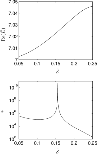
Figure 1: Stabilization effect for one of the electric-field-induced impurity states.

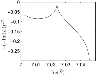
Figure 2: Path of the Green’s function pole with a changing electric field.

As has been expected, for the vanishing point interaction, i.e. when $\tilde{E}_{B}=0$, the exact Green’s function reduces to the Green’s function for electrons moving only in crossed magnetic and electric fields. Zeros of $\tilde{D}(\tilde{E})$ determine complex energies of those resonances which are induced by the presence of an impurity described by an attractive point interaction. On top of that, the exact Green’s function allows us to establish unambiguously the exact form of the wavefunctions for such a resonance provided that it is not degenerate. Indeed, if $E_{\mathrm{r}}$ is the resonance energy, hence the wavefunctions are defined by the relation (not in our scaled units)

$$\lim_{E\rightarrow E_{\mathrm{r}}}(E-E_{\mathrm{r}})G(\mathbf{r},\mathbf{r}^{\prime};E)=\psi_{\mathrm{r}}(\mathbf{r})[\psi^{A}_{\mathrm{r}}(\mathbf{r}^{\prime})]^{*}\,.$$ (4)

At this point it is crucial to stress that for resonances, in contrast to the bound state problem, there exist two wavefunctions which we call the retarded $\psi_{\mathrm{r}}(\mathbf{r})$ and the advanced $\psi^{A}_{\mathrm{r}}(\mathbf{r})$ wavefunctions (see also F87 ; Reson ; MFSF00 ). For these functions the normalization condition has the form

$$\int\,\mathrm{d}\mathbf{r}\,\psi_{\mathrm{r}}(\mathbf{r})[\psi^{A}_{\mathrm{r}}(\mathbf{r})]^{*}=1\,.$$ (5)

It turns out that for an infinitely long-living resonance, i.e. when the energy becomes real, both these wavefunctions are identical. This property is exemplified by our model. Defining, in our scaled units, the un-normalized retarded and advanced wavefunctions as

$$\tilde{\psi}_{\mathrm{r}}(\tilde{\mathbf{r}})=-\mathrm{i}\,\tilde{G}_{0}(\tilde{\mathbf{r}},\mathbf{0};\tilde{E}_{\mathrm{r}})\,,$$ (6)

and

$$[\tilde{\psi}^{A}_{\mathrm{r}}(\tilde{\mathbf{r}})]^{*}=\mathrm{i}\,\tilde{G}_{0}(\mathbf{0},\tilde{\mathbf{r}};\tilde{E}_{\mathrm{r}})\,,$$ (7)

one can prove that

$$\int\,\mathrm{d}\tilde{\mathbf{r}}\,\tilde{\psi}_{\mathrm{r}}(\tilde{\mathbf{r}})[\tilde{\psi}^{A}_{\mathrm{r}}(\tilde{\mathbf{r}})]^{*}=\frac{\partial\tilde{D}(\tilde{E})}{\partial\tilde{E}}\mid_{\tilde{E}=\tilde{E}_{\mathrm{r}}}=\tilde{D}^{\prime}(\tilde{E}_{\mathrm{r}})\,.$$ (8)

Hence, in the close vicinity of a resonance, where $\tilde{D}(\tilde{E}_{\mathrm{r}})=0$, we get the following relation

$$\tilde{G}(\tilde{\mathbf{r}},\tilde{\mathbf{r}}^{\prime};\tilde{E})\cong\frac{1}{\tilde{E}-\tilde{E}_{r}}\frac{\tilde{\psi}_{\mathrm{r}}(\tilde{\mathbf{r}})[\tilde{\psi}^{A}_{\mathrm{r}}(\tilde{\mathbf{r}}^{\prime})]^{*}}{\tilde{D}^{\prime}(\tilde{E}_{\mathrm{r}})}\,,$$ (9)

which agrees with (4) and (5). Furthermore, for real $\tilde{E}_{\mathrm{r}}$ both $\tilde{\psi}_{\mathrm{r}}(\tilde{\mathbf{r}})$ and $\tilde{\psi}^{A}_{\mathrm{r}}(\tilde{\mathbf{r}})$ are identical, which we have also checked numerically.

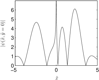
Figure 3: Modulus of $\psi(\tilde{x},\tilde{y}=0)$ for the stable resonance.

We have already pointed out in KK1 that the electric-field-induced resonances exhibit peculiar behavior with an increasing electric field strength. Namely, for some particular values of electric fields and binding energies the lifetime of these states (within a computational error) can be infinite, i.e., we observe the stabilization process. We have checked that this phenomenon cannot happen for the ’old’ localized impurity-induced states already discussed in GM99 ; CC98 . For this reason let us consider the electric-field-induced resonances located near the third excited Landau level of the scaled energy $\tilde{E}=7$. There are three such states and the stabilization phenomenon for one of them is presented in Fig. 1. It happens for the scaled electric field $\tilde{\mathcal{E}}=0.1555$ and binding energy $\tilde{E}_{B}=-6.4$ (for other values of these parameters a very similar behavior occurs for the remaining two resonances, therefore, we shall not attach the corresponding figures here). In Fig. 2 we present positions of energies in the complex energy plane for this resonance with changing electric field. For the visual purpose we have raised the imaginary part of this energy to the power $1/5$. We observe that initially an increasing electric field tears off the resonance energy from the Landau level (as it has been demonstrated in KK1 ) and pushes it down. However, with a still increasing electric field strength the energy starts migrating back towards the real axis and approaches it, within a numerical error, for some particular value of $\tilde{\mathcal{E}}$, for which the lifetime of this resonance becomes infinite. For still larger electric fields the energy again, as expected, withdraws downwards from the real axis. What is the reason for this peculiar behavior? In order to answer this question we have analyzed the wavefunction of this resonance. We present in Fig. 3 the wavefunction for $\tilde{y}=0$ when the stabilization takes place. It is clearly seen that at the origin $\tilde{\mathbf{r}}=\mathbf{0}$, where the impurity is located, the wavefunction is singular and one can prove by analyzing equation (6) that this singularity is of the logarithmic type. However, more interesting is that the wavefunction posses five zeros which are attributed to quantum-mechanical vortices, as it will follow below. This means that responsible for the stabilization effect is the particular vortex-type motion of the ‘probability fluid’ and, hence, induced by such a motion quantum-mechanical interferences.

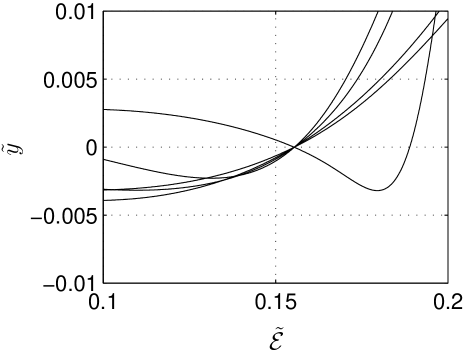
Figure 4: $\tilde{y}$-coordinates of vortices as functions of the electric field strength.

III Vortices

It is well-known that the magnetic field induces quantum-mechanical vortices and that the circulation around them is quantized BCK92 ; BBS00 . The same phenomenon occurs in our model, except the fact that instead of the vortex line for three-dimensional space we have the vortex point for two dimensions. Moreover, it turns out that the electric field can be used as a control parameter with the help of which one can change the positions of these vortices. In particular, it might happen that for some values of the electric field strength all these vortices can be aligned along the axis defined by the direction of the electric field vector, in our case along the $x$-axis. If this takes place the stabilization occurs, i.e., the electric field is not able to push out the electron from the vicinity of an impurity. In order to show this we have determined zeros of the wavefunction $\tilde{\psi}(\tilde{\mathbf{r}})$ for $\tilde{E}_{B}=-6.4$ and for different electric field strengths. The $\tilde{y}$-coordinates of five zeros for the resonance state considered above are presented in Fig. 4. We see that they cross the $\tilde{x}$-axis exactly for such an electric field for which the stabilization appears. Moreover, in Table 1 we present the $\tilde{x}$-coordinates of these vortices for this particular electric field. The path in the coordinate plane of the vortex number 3 from Table 1 is displayed in Fig. 5. We observe that for small electric fields this vortex is located just below the $\tilde{x}$-axis and for a particular electric field strength it crosses this axis (at this moment the lifetime goes to infinity) and afterwards runs away from the impurity center in the perpendicular direction to the electric field vector. The very similar behavior appears for the remaining four vortices. These numerical findings show that the alignment of all vortices along the $\tilde{x}$-axis is the reason for the stabilization phenomenon observed in Figs. 1 and 2.

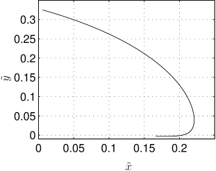
Figure 5: Path in the coordinate plane of a vortex for different values of $\tilde{\mathcal{E}}$.

In order to get more insight into the vortex structure of stable resonances we have to investigate the phase of the wavefunction and probability current. Since for stable resonances the retarded and advanced wavefunctions are identical, therefore, it is sufficient to explore the phase of only one of them. We define the phase $S(\tilde{\mathbf{r}})$ by the equation

$$\tan\bigl{(}S(\tilde{\mathbf{r}})\bigr{)}=\frac{\mathrm{Im}(\tilde{\psi}(\tilde{\mathbf{r}}))}{\mathrm{Re}(\tilde{\psi}(\tilde{\mathbf{r}}))}\,,$$ (10)

with the assumption that $-\pi<S(\tilde{\mathbf{r}})\leqslant\pi$. The scaled probability current is equal to

$$\tilde{\mathbf{j}}(\tilde{\mathbf{r}})=\mathrm{Im}\bigl{(}\tilde{\psi}^{*}(\tilde{\mathbf{r}})(\tilde{\mathbf{\nabla}}-{\rm i}e\tilde{\mathbf{A}}(\tilde{\mathbf{r}}))\tilde{\psi}(\tilde{\mathbf{r}})\bigr{)}\,,$$ (11)

where both $\tilde{\mathbf{\nabla}}$ and $\tilde{\mathbf{A}}$ are scaled the nabla operator and vector potential. This current defines the scaled probability velocity $\tilde{\mathbf{v}}(\tilde{\mathbf{r}})$ BCK92 ; BBS00

$$\tilde{\mathbf{j}}(\tilde{\mathbf{r}})=(\tilde{\mathbf{v}}(\tilde{\mathbf{r}})-e\tilde{\mathbf{A}}(\tilde{\mathbf{r}}))\mid\!\tilde{\psi}(\tilde{\mathbf{r}})\!\mid^{2}\,,$$ (12)

which has to fulfil the quantization condition

$$\Gamma_{C}=\oint_{C}\tilde{\mathbf{v}}(\tilde{\mathbf{r}})\cdot\mathrm{d}\tilde{\mathbf{r}}=2\pi N\,,$$ (13)

where $C$ is an arbitrary contour in the $\tilde{x}\tilde{y}$-plane and $N$ is an integer number. We have checked in our numerical investigations that within a numerical error the foregoing quantization condition is fulfilled by any contour in the $\tilde{x}\tilde{y}$-plane. In particular, by choosing as a contour small circles encircling only one vortex we have calculated circulations for five vortices appearing for this state (see, Table 1). We see that three of them have positive circulations (we call them vortices), whereas the remaining two negative ones (we call them anti-vortices). It is interesting to notice that an anti-vortex appears in the pair with a vortex. This fact is presented in Fig. 6 where the contour plot of the phase is drawn. We clearly see in this plot five vortices located on the $\tilde{x}$-axis with the $\tilde{x}$-coordinates collected in Table 1. In this figure three arrows indicate three bold lines which correspond to the discontinuity of the phase, where the phase suddenly changes its value by $\pm 2\pi$. We see that the vortex and anti-vortex are always connected by such a discontinuity line, whereas for the remaining third vortex this line escapes to the infinity. The quiver plot of the probability velocity vector $\tilde{\mathbf{v}}(\tilde{\mathbf{r}})$ near this vortex is presented in Fig. 7. It is shown that the magnitude of $\tilde{\mathbf{v}}(\tilde{\mathbf{r}})$ becomes larger in the closer vicinity of the vortex point. Such a behavior guarantees that the circulation $\Gamma_{C}$ is preserved indeed, i.e., the quantization condition (13) holds for any closed contour encircling the vortex.

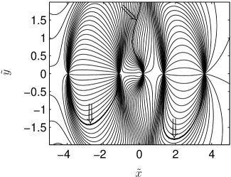
Figure 6: Contour plot of the phase of the wavefunction for the stable resonance.

Table 1: Positions of five vortices and their circulations.

vortex	$\tilde{x}\quad\quad$	$\Gamma_{C}/2\pi$
1	$-$3.943428	$-$1
2	$-$1.148087	$+$1
3	0.216306	$+$1
4	1.347754	$+$1
5	3.610649	$-$1

To summarize, we have shown that for the electric-field-induced impurity states there exist some particular values of $\tilde{\mathcal{E}}$ and $\tilde{E}_{B}$ for which the stabilization phenomenon occurs and that this effect is directly connected with quantum-mechanical vortices which, for these stabilized resonances, are all placed along the $\tilde{x}$-axis. We have discussed this problem for one particular resonance, but our findings are generally valid for all other states in the sense that we have checked this for states located in the vicinity of excited Landau levels of the principal quantum numbers $n=1$, 2 and for the case of $n=3$, studied in this paper. The stabilization effect does not appear for impurity states discussed previously in CC98 ; GM99 . It also appears that the number of vortices present in these states is equal to $2n-1$.

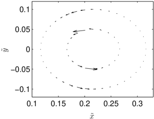
Figure 7: Quiver plot of the probability velocity for the stable resonance and for two chosen contours.

- (1) N. Berglund, A. Hansen, E. H. Hauge, J. Piasecki, Phys. Rev. Lett. 77 (1996) 2149.
- (2) E. H. Hauge, J. M. J. van Leeuwen, Physica A 268 (1999) 525.
- (3) S. Gyger, P. A. Martin, J. Math. Phys. 40 (1999) 3275.
- (4) K. Krajewska, J. Z. Kamiński, quant-ph/0205106.
- (5) R. M. Cavalcanti, C. A. A. de Carvalho, J. Phys. A 31 (1998) 2391.
- (6) F. H. M. Faisal, Theory of Multiphoton Processes, New York, 1987.
- (7) V. I. Kukulin, V. M. Krasnopol’sky, J. Horáček, Theory of Resonances. Principles and Applications, Kluwer Akademic Publishers, Prague, 1989.
- (8) N. L. Manakov, M. V. Frolov, A. F. Starace, I. I. Fabrikant, J. Phys. B 33 (2000) R141.
- (9) I. Białynicki-Birula, M. Cieplak, J. Kamiński, Theory of Quanta, Oxford University Press, New York, 1992.
- (10) I. Białynicki-Birula, Z. Białynicka-Birula, C. Śliwa, Phys. Rev. A 61 (2000) 032110.