Entanglement between two macroscopic fields by coherent atom-mediated exchange of photons

Abstract

Using two different criteria for continuous variable systems we demonstrated that pump and probe beams became quantum correlated in a situation of Electromagnetically Induced Transparency in a sample of ⁸⁵Rb atoms. Our result combines two important features for practical implementations in the field of quantum information processing. Namely, we proved the existence of entanglement between two macroscopic light beams, and this entanglement is intrinsically associated to a strong coherence in an atomic medium.

In the last two decades, the philosofical and technological impacts of quantum correlations or entanglement in multipartite physical systems have been accentuated by the theoretical and experimental investigations leading to the development of the area of quantum information processing bennett . The existence of entanglement, which is an evidence of the non-local character of the quantum theory, has been confirmed in quantum optics experiments using dichotomics aspect and continuous variable systems kimble1 . These experimental realizations made possible some implementations in the fields of quantum information kimble ; gisin and computation haroche1 ; ions . Even so, the unavoidable interaction between the physical system used to process the quantum information and the environment leads to a loss of coherence, and consequently, to a loss of information that introduces important limitations to the practicality of the quantum information processing technology. Since it is impossible to have isolated systems, among the different approaches employed to reduce the influence of the environment we find the use of continuous variable systems, specifically, intense light beams as in the case of quantum teleportation based on the entanglement between twin beams issued from an OPO kimble . In that sense, there are propositions, for exemple, for quantum cryptography ralph , quantum computation lloyd , dense coding samuel , and quantum key distribution leuchs . Another approach is to use coherently-prepared atomic media and, in this case, the Electromagnetically Induced Transparency (EIT) is a good candidate as it has been demonstrated recently by the observation of very slow light pulse propagation paq and light storage p . In this context, a natural question arises: can we produce entanglement between two intense ligth beams in a coherently-prepared atomic medium, combining in that way the two mentioned approaches? As we will see through out this paper, the answer to this question is yes and this result is very important due to the recent huge interest in the applications of coherently-prepared atomic media using EIT mastko .

In this paper, we show that three-level atoms can produce entanglement in two intense travelling light fields, in the EIT regime. We study this system from a theoretical point of view, and we show that for some particular parameters, the two fields present quantum correlations after interacting with the atoms, even if they are initially completely uncorrelated. We demonstrate the existence of entanglement between these two propagating fields according to two different criteria.

In our model, we consider three-level atoms in a closed $\Lambda$ configuration (ground states $|1\rangle$ and $|2\rangle$, and excited state $|0\rangle$) interacting with two copropagating fields treated quantum-mechanically. In the Heisenberg picture, the electric field operator for the propagating mode $j$ (pumping laser $j=1$, probe laser $j=2$) is given by the expression

$$\widehat{\vec{E}}_{j}(t)={\cal E}_{0\omega_{Lj}}\bar{\epsilon}_{j}e^{-i\omega_{Lj}t}\hat{A}_{j}(t)+h.c.\ ,$$ (1)

where ${\cal E}_{0\omega_{Lj}}$ , $\bar{\epsilon}_{j}$ and $\omega_{Lj}$ are the amplitude, the polarization direction and the angular frequency of mode (laser) $j$, respectively. $\hat{A}_{j}$ ($\hat{A}^{{\dagger}}_{j}$) is the annihilation (creation) operator and represents the slowly varying amplitude of the laser field. We take the hamiltonian

$$\hat{H}_{Lj}=\int_{-\infty}^{+\infty}d\omega\ |G_{j}(\omega)|^{2}\hbar\omega\ \hat{a}^{{\dagger}}_{j\omega}\hat{a}_{j\omega}\$$ (2)

as the energy source of the interacting field where, $\hat{a}_{j\omega}$ is the annihilation operator of the field inside the laser source cavity and, through the non-dimensional function $G_{j}(\omega)$, we take into account the influence of the external vacuum modes. This function is determined by the frequency-dependent reflectivity of the output mirror of the laser cavity and provides the laser linewidth $\gamma_{j}$, which we assume to be constant here, in accordance with the Markov approximation gardiner . Taking into account the theoretical and experimental studies about the laser sources, we took $G_{j}(\omega)$ as a lorentzian profile centered at the laser frequency $\omega_{Lj}$, allowing the lower integration limit in (2) be taken equal to $-\infty$ instead of zero.

The coupling between the source and the propagating mode is given by the linear hamiltonian

$$\hat{H}_{Lj-Cj}=i\hbar\sqrt{\frac{\gamma_{j}}{2\pi}}\int_{-\infty}^{+\infty}d\omega\ \hat{a}^{{\dagger}}_{j\omega}\hat{A}_{j}(t)+h.c.$$ (3)

We obtain the interaction hamiltonian for the two light beams and the atoms, within the usual dipole and rotating-wave approximations

$$\hat{H}_{int}=\hbar g_{1}\hat{S}^{+}_{1}(t)\hat{A}_{1}(t)+\hbar g_{2}\hat{S}^{+}_{2}(t)\hat{A}_{2}(t)+h.c.\ ,$$ (4)

where $g_{1}$ ($g_{2}$) is the atom – field 1 (field 2) coupling strength, and $\hat{S}^{+}_{1}$ ($\hat{S}^{+}_{2}$) the slowly varying envelope of the atomic polarization on the transition $|1\rangle\leftrightarrow|0\rangle$ ($|2\rangle\leftrightarrow|0\rangle$).

The dynamics of the system is determined by twelve coupled quantum Langevin equations derived from the Heisenberg equations of motion. Since we are dealing with macroscopic systems, the quantum fluctuations of the operators are studied by linearizing them around their steady-state values and the dynamics of these fluctuations is described by a matrix linear stochastic differential equation for the fluctuation operators tobe . Recently, intensity correlations between the pump and probe fields in EIT have been measured exper . These can be understood by inspection of the equations for the fluctuations of one field and for the corresponding atomic polarization:

$$\frac{d\delta\hat{A}_{1}(t)}{dt}=-\frac{\gamma_{1}}{2}\delta\hat{A}_{1}(t)-ig_{1}\delta\hat{S}^{-}_{1}(t)+\sqrt{\gamma_{1}}\delta\hat{A}_{1in}(t)\ ,$$ (5)

$$\frac{d\delta\hat{S}^{-}_{1}(t)}{dt}=-\left(\frac{\Gamma_{1}+\Gamma_{2}}{2}-i\ \delta_{L1}\right)\delta\hat{S}^{-}_{1}(t)$$

$$+ig_{1}w_{1}\delta\hat{A}_{1}(t)+ig_{1}\alpha_{1}\delta\hat{W}_{1}(t)$$

$$-ig_{2}s^{*}_{12}\delta\hat{A}_{2}(t)-ig_{2}\alpha_{2}\delta\hat{S}^{{\dagger}}_{12}(t)+\hat{F}_{S1}(t)\;.$$ (6)

Here we define $\hat{A}_{1in}$ the annihilation operator of the source or input field 1, $\Gamma_{1}$ ($\Gamma_{2}$) the spontaneous emission rate from $|0\rangle\rightarrow|1\rangle$ ($|0\rangle\rightarrow|2\rangle$), $\delta_{L1}$ the detuning between field 1 and the corresponding atomic transition, $w_{1}$ the steady-state inversion between states $|0\rangle$ and $|1\rangle$, $\alpha_{1}$ ($\alpha_{2}$) the steady-state amplitude of field 1 (field 2), $\hat{W}_{1}$ the inversion (operator) between states $|0\rangle$ and $|1\rangle$, $s^{*}_{12}$ the steady-state coherence between ground states $|1\rangle$ and $|2\rangle$, $\hat{S}^{+}_{12}$ the coherence operator, $\hat{F}_{S1}$ the Langevin fluctuation force. The notation $\delta\hat{S}^{-}_{1}$ means fluctuations of the corresponding operator. The fluctuations of the input $\delta\hat{A}_{1in}$, the interacting $\delta\hat{A}_{1}$ and the detected $\delta\hat{A}_{1out}$ fields are related by the expression $\delta\hat{A}_{1out}=\delta\hat{A}_{1in}-\sqrt{\gamma_{1}}\delta\hat{A}_{1}$.

From Eq. (6), we notice that noise correlations between the fields are created, owing to the coherent effect in the atomic medium exper . In Fig. 1 we show the quadrature correlations of the fields in the frequency domain as a function of probe detuning for a resonant pump. This theoretical prediction (and the following too) corresponds to a system of N=$10^{8}$ atoms of ⁸⁵Rb where the states of the $\Lambda$ configuration are designated as follows: $|0\rangle=|5P_{3/2},F^{{}^{\prime}}=3\rangle$, $|1\rangle=|5S_{1/2},F=3\rangle$ and $|2\rangle=|5S_{1/2},F=2\rangle$. The pump and probe lasers are taken linearly polarized with equal intensities (2.8 mW/cm²) and issued from two independent sources with quantum fluctuations corresponding to a coherent state. We took the analysis frequency $\Omega=\Gamma/6$, where $\Gamma=\Gamma_{1}+\Gamma_{2}=2\pi\ 6$ MHz is the total decay rate of the rubidium excited state. The correlation, taking values in the interval [-1;1], is defined as the ratio between the fields covariance and the squared root of the product of the fields’ variances. Outside the EIT window the fields are completely uncorrelated and, in the EIT condition (zero probe detuning), there is the following correlation between the fluctuations of the fields quadratures: $\delta\hat{Y}_{1out,0}\leftrightarrow\delta\hat{Y}_{2out,0}$ and $\delta\hat{Y}_{1out,\pi/2}\leftrightarrow-\delta\hat{Y}_{2out,\pi/2}$. The subscript 0 ($\pi/2$) stands for the field amplitude (phase) quadrature and the general quadrature fluctuation operator is, for the field 2, given by $\delta\hat{Y}_{2out,\phi}(t)=\delta\hat{A}_{2out}(t)e^{-i\phi}+\delta\hat{A}^{{\dagger}}_{2out}(t)e^{i\phi}$.

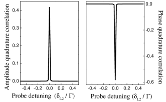
Figure 1: Correlation between amplitude and phase quadratures.

The observed correlations can be interpreted from the propagation dynamics of the beams. When the beams have the same intensity, the role “pump” and “probe” is interchangeable and for a resonant coupling of both fields the atomic medium presents exactly the same absorptive and dispersive responses for these beams. This regime, that may be called electromagnetically mutual induced transparency (EMIT), is broken down when we introduce a detuning in one of the fields, creating in this way a phase difference between them leading to their decorrelation.

We use two criteria for continuous variable systems to distinguish between quantum and classical correlations. We begin our analysis with the criterion of the inferred variances, described theoretically in reid and experimentally implemented in kimble1 ; kimble . Let us suppose that we are interested in the inferrence of the probe field amplitude ($\phi=0$) and phase ($\phi=\pi/2$) quadratures from measurements of the pump field quadratures. In this case, the inferred variances of the probe quadratures are defined by the equations

$$\Delta^{2}_{inf}Y_{2,0}(t)\equiv\langle\Big{(}\hat{Y}^{{}^{\prime}}_{2out,0}(t)-\eta_{0}\ \hat{Y}^{{}^{\prime}}_{1out,0}(t)\Big{)}^{2}\rangle\ ,$$ (7)

$$\Delta^{2}_{inf}Y_{2,\pi/2}(t)\equiv\langle\Big{(}\hat{Y}^{{}^{\prime}}_{2out,\pi/2}(t)+\eta_{\pi/2}\ \hat{Y}^{{}^{\prime}}_{1out,\pi/2}(t)\Big{)}^{2}\rangle\ ,$$ (8)

where $\hat{Y}^{{}^{\prime}}_{jout,0}(t)=\hat{Y}_{jout,0}(t)-\langle\hat{Y}_{jout,0}(t)\rangle$ and $\hat{Y}^{{}^{\prime}}_{jout,\pi/2}(t)=\hat{Y}_{jout,\pi/2}(t)-\langle\hat{Y}_{jout,\pi/2}(t)\rangle$ with $j=1,2$. The parameters $\eta_{0}$ and $\eta_{\pi/2}$ take into account the non-perfect correlation between the fields and the non-ideal efficiency of the measurement procedure. The values of these parameters are taken in order to minimize the inferred variances (7) and (8), allowing the following criterion, in the frequency domain, for the entanglement of the pump and probe fields

$$[\Delta^{2}_{inf}Y_{2,0}(\Omega)]_{min}[\Delta^{2}_{inf}Y_{2,\pi/2}(\Omega)]_{min}<1\ .$$ (9)

That is to say, if the product of the inferred variances is less than 1, then the correlation between the fields has a quantum nature. In Fig. 2 we show the product of the inferred variances for the probe field. As expected, outside de EIT region, the inequality (9) is violated since the fields are uncorrelated (see Fig. 1). However, in the EIT condition, the pump and probe fields became quantum correlated.

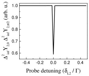
Figure 2: Product of the minimal inferred variances of the probe field.

The other criterion used to establish the nature of the fields correlation is the theorem of Duan et al. zoller , which we will abreviate as DGCZ. Taking $a=1$, introducing the equivalence between the fields quadrature operators and the operators defined in zoller as $\hat{x}_{1}\Leftrightarrow\hat{Y}_{1out,0}$, $\hat{p}_{1}\Leftrightarrow\hat{Y}_{1out,\pi/2}$, $\hat{x}_{2}\Leftrightarrow\hat{Y}_{2out,0}$ and $\hat{p}_{2}\Leftrightarrow\hat{Y}_{2out,\pi/2}$, and using the commutation relation $[\hat{x}_{j},\hat{p}_{j^{{}^{\prime}}}]=2i\delta_{jj^{{}^{\prime}}}$ derived from the definition of the quadrature operators, we find the following necessary condition to prove that the join state of the pump and probe fields is separable

$$\langle(\Delta\hat{u})^{2}\rangle_{\rho}+\langle(\Delta\hat{v})^{2}\rangle_{\rho}\geq 4\ .$$ (10)

Since this last inequality provides a necessary condition for the separability of the join fields state, then its violation is a sufficient condition for the inseparability or entanglement between the fields. In Fig. 3 we plot the left hand side of the inequality (10) and, again, outside the EIT window the equality is satisfied since the fields are uncorrelated. In the EIT condition, the violation of (10) indicates that the pump and probe fields are entangled. We must point out that both criteria report about 40 % of entanglement of the fields. This amount of quantum correlation is limited by the decay rate of the coherence between the two ground states.

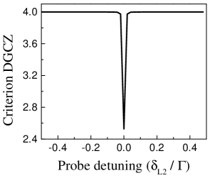
Figure 3: Pump-probe entanglement according to the DGCZ criterion.

The predicted quantum correlation between the pump and probe fields in the EIT condition is associated to the existence of phase quadrature squeezing in both fields. This squeezing, produced in the coherent situation, depends on the intensities of the source fields and, as it can be observed from the bistability response of the detected fields, it is produced at the turning point of the bistability curve and is accompanied by an excess noise in the corresponding conjugate quadrature amplitude tobe .

These results may be somehow unexpected because it is believed that in the EIT condition the field fluctuations are not altered for field intensities higher or comparable to the saturation intensity of the atomic transition. As we showed theoretically and experimentally exper this is not the case. In the EIT situation there is a coherent atom-mediated exchange of photons between the pump and probe fields that preserves their mean intensities and at the same time modifies their quantum noise properties creating a correlation between them. This modification of the field quantum fluctuations is a direct consequence of the strong coherence induced in the atomic medium by the two beams.

So far, the correlation properties of the pump and probe beams have not been extensively studied in the EIT experiments. Entanglement between two single-photon pulses (quantum fields) has been predicted before in a coherently-prepared medium by two classical beams lukin . In this paper, we show that the same intense beams used to prepare the transparent nonlinear medium, in particular circumstances, become entangled even when the investigated system is subjet to the influence of a reservoir and consequently the quantum correlations are predicted in a system that is not “pure”. Since we demonstrated the existence of entanglement between the light beams only, our result suggests that there exists stronger quantum correlations in the system atom – pump field – probe field. Another remarkable point is that the investigation of the correlations and quantum fluctuations of the light beams in the EIT situation provides a precise tool to determine the natural width of the EIT resonance, and this can be a very powerful method to attain the highest sensibility in detecting coherent effects in atomic media.

Given the possible technological applications of such intense entangled fields, it is our understanding that the statistical properties of these fields deserve further experimental investigations in the near future. Not only do they open the possibility to use such systems as a macroscopic resource for different quantum technologies, but they also help understanding the nature of entanglement and how it may arise from non-linear couplings in macroscopic media.

Finally, in Fig. 4 we present an experimental setup that can be employed to measure the entanglement between the pump and probe fields. Considering the light beams have orthogonal polarizations, they can be separated using polarizing cube beam splitters and then the variance of their quadratures and the correlation between them can be determined utilizing homodyne detectors. From practical considerations, the analysis frequency must be chosen as low as possible since in this case we have more sensibility to detect correlated photons.

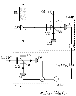
Figure 4: Experimental setup to measure the probe field inferred variances. PBS: polarizing cube beam splitter; $\lambda/2$: half-wave plate; D1, D2, D3, and D4: photodetectors; OL1($\theta$) and OL2($\phi$): local oscillators for the pump and probe field, respectively; $\eta_{0}(\eta_{\pi/2})$: controlled-gain amplifier for the amplitude (phase) quadrature.

M.F.S. would like to thank Prof. S. Salinas for his hospitality at the University of São Paulo. The authors acknowledge the financial support of the Brazilian agencies CAPES, FAPESP and CNPq.

References

- (1) Present address: Blackett Laboratory, Imperial College, London SW7 2BW, United Kingdom.
- (2) See, for exemple, C. H. Bennett, Phys. Today 48(10), 24 (1995); C. H. Bennett, G. Brassard, and A. K. Ekert, Sci. Am. 267(4), 50 (1992).
- (3) See, for exemple, A. Aspect, J. Dalibard, and G. Roger, Phys. Rev. Lett. 49, 1804 (1982).
- (4) Z. Y. Ou, S. F. Pereira, H. J. Kimble, and K. C. Peng, Phys. Rev. Lett. 68, 3663 (1992).
- (5) A. Furusawa et al., Science 282, 706 (1998).
- (6) A. Muller, H. Zbinden, and N. Gisin, Europhys. Lett. 33, 335 (1996).
- (7) P. Domokos et al., Phys. Rev. A 52, 3554 (1995).
- (8) C. Monroe et al., Phys. Rev. Lett. 75, 4714 (1995).
- (9) T. C. Ralph, quant-ph/9907073.
- (10) S. Lloyd and S. Braunstein, Phys. Rev. Lett. 82, 1784 (1999).
- (11) S. Braunstein and H. J. Kimble, quant-ph/9910010.
- (12) Ch. Silberhorn, N. Korolkova, and G. Leuchs, Phys. Rev. Lett. 88, 167902 (2002).
- (13) L. V. Hau et al., Nature (London) 397, 594 (1999); M. M. Kash et al., Phys. Rev. Lett. 82, 5229 (1999); D. Budker et al., Phys. Rev. Lett. 83, 1767 (1999).
- (14) C. Liu et al., Nature (London) 409, 490 (2001); D. F. Phillips et al., Phys. Rev. Lett. 86, 783 (2001).
- (15) A. S. Zibrov et al., Phys. Rev. Lett. 88, 103601 (2002).
- (16) C. W. Gardiner, “Quantum Noise”, Springer-Verlag (1991).
- (17) C.L. Garrido Alzar, Ph. D. thesis, University of São Paulo, 2002.
- (18) C.L. Garrido Alzar et al., quant-ph/0204060.
- (19) M. D. Reid, Phys. Rev. A 40, 913 (1989).
- (20) L.-M. Duan et al., Phys. Rev. Lett. 84, 2722 (2000).
- (21) M. D. Lukin and A. Imamoğlu, Phys. Rev. Lett. 84, 1419 (2000); ibid., Nature (London) 413, 273 (2001); M. D. Lukin et al., Phys. Rev. Lett. 84, 4232 (2000) .