Decoherence scenarios from micro- to macroscopic superpositions

Abstract

Environment induced decoherence entails the absence of quantum interference phenomena from the macroworld. The loss of coherence between superposed wave packets is a dynamical process the speed of which depends on the packet separation: The farther the packets are apart, the faster they decohere. The precise temporal course depends on the relative size of the time scales of decoherence and other processes taking place in the open system and its environment. We use the exactly solvable model of an harmonic oscillator coupled to a bath of harmonic oscillators to illustrate various decoherence scenarios: These range from exponential golden-rule decay for microscopic superpositions, system-specific decay for larger separations in a crossover regime, and finally the universal interaction-dominated decoherence for ever more macroscopic superpositions investigated in great generality in the accompanying paper [W. T. Strunz, F. Haake, and D. Braun; Phys. Rev. A, henceforth referred to as [SHB]].

I Introduction

A collection of $N+1$ harmonic oscillators $N$ of which are mutually free but all coupled, symmetrically and harmonically, to the remaining oscillator, enjoys considerable popularity as a model of an $N$-freedom environment acting on a single-freedom system generalosci ; masterosciref . The importance of the model lies in its rigorous explicit tractability through a normal-mode analysis. Most applications aim at revealing the effectively irreversible behavior of the central oscillator brought about by the coupling to the environment (alias “bath”) for large $N$; in the limit $N\to\infty$ even strict irreversibility results under certain assumptions for the distribution of bath frequencies, and the central oscillator becomes linearly damped.

While obliged to the tradition just pointed to, the present paper picks up a more recent trend and exploits the rigorous tractability of the model to reveal the emergence of classical behavior from quantum dynamics in the passage from the microscopic to the macroscopic world Zeh ; Zurek ; Habib . In particular, we study the temporal fate of superpositions of two wave packets for the central oscillator as in Habib , yet concentrate on the various decoherence scenarios emerging as the distance of the superposed wave packets is varied from microscopic to macroscopic scales. As is by now well known such superposed packets loose their relative coherence, due to the dissipative influence of the bath, the faster the larger the initial separation of the two wave packets. The life time $\tau_{\rm dec}$ of the relative coherence is inversely proportional to a power of the initial separation, $\tau_{\rm dec}\propto(\lambda/d)^{\nu}$ with $\nu>0$; within the power law, the separation $d$ is referred to a microscopic quantum scale $\lambda$, and therefore exceedingly rapid decoherence results as $d$ is increased towards macroscopic magnitude. Keeping all other parameters of the problem fixed, it is the initial separation between the two wave packets only that determines the size of the decoherence time scale $\tau_{\rm dec}$ relative to other relevant system or environmental time scales.

The most familiar golden-rule limit

$$\tau_{\rm sys}\ll\tau_{\rm dec}\ll\tau_{\rm diss}\,,$$ (1)

which allows the system to undergo many cycles during decoherence, can hold only as long as the separation between the two wave packets remains below a certain limit. On increasing the separation we encounter a qualitatively different regime in which decoherence is faster than any system time scale,

$$\tau_{\rm dec}\ll\tau_{\rm sys},\tau_{\rm diss},$$ (2)

irrespective of the relative size of $\tau_{\rm sys}$ and $\tau_{\rm diss}$. In that interaction dominated limit the free-motion Hamiltonian of the central oscillator, rather than the interaction with the bath, behaves like a weak perturbation during decoherence. For yet larger separations decoherence becomes the fastest process by far, faster even than reservoir time scales,

$$\tau_{\rm dec}\ll\tau_{\rm res},\tau_{\rm sys},\tau_{\rm diss}\,.$$ (3)

The universal behavior resulting in the limit (3) may look like instantaneous decoherence on the classical time scales $\tau_{\rm sys},\tau_{\rm diss}$. While certainly requiring separations $d$ huge on the quantum scale $\lambda$, the limit (3) will turn out to allow, surprisingly, moderate or even small $d$ relative to every-day macroscopic scales.

The pure limiting cases mentioned above allow for analytical treatment for general open systems, as shown in the accompanying paper [SHB]. Crucially, decoherence in the interaction dominated cases (2) or (3) becomes independent of the system Hamiltonian and may thus be regarded as the origin of the universally observed absence of quantum interferences in the macroworld. All of these general findings of the accompanying paper will be illustrated for the oscillator model here. However, the principal purpose of the present paper is to study the interesting crossovers between the three regimes mentioned; since these crossover effects elude the general asymptotic methods of [BHS], the exact tractability of the oscillator model allows precious insights into the emergence of classical behavior.

II Decoherence of superposed wave packets

We illustrate the various decoherence scenarios for a superposition of Gaussian wave packets

$$|\varphi\rangle=c_{1}|\varphi_{1}\rangle+c_{2}|\varphi_{2}\rangle\,,\quad|c_{1}|^{2}+|c_{2}|^{2}=1.$$ (4)

In the position representation,

$$\langle q|\varphi_{i}\rangle=\varphi_{i}(q)=\frac{1}{(2\pi\sigma)^{1/4}}\,{\rm e}^{{\rm i}p_{i}(q-q_{i})/\hbar}\,{\rm e}^{-(q-q_{i})^{2}/4\sigma}$$ (5)

with $\quad i=1,2\,$. These packets are located in position space at $q_{i}$ with (rms) uncertainty $\Delta q=\sqrt{\sigma}$ and in momentum space at $p_{i}$ with uncertainty $\Delta p=\hbar/2\sqrt{\sigma}$. We choose coherent states Glauber with the minimum uncertainty $\Delta q\Delta p=\hbar/2$ such that both $\Delta q$ and $\Delta p$ are $\propto\sqrt{\hbar}$. To ensure good separation we stipulate that either $\Delta q\ll|q_{1}-q_{2}|$ or $\Delta p\ll|p_{1}-p_{2}|$ or both (see Fig. 1).

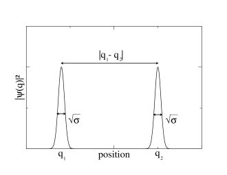
Figure 1: Position space density $|\psi(q)|^{2}$ for a superposition of two Gaussian wave packets with mutual distance much larger than individual spread.

The initial density operator corresponding to the state (4) is a sum of four terms,

$$\rho_{\rm sys}(0)=\sum_{i,j=1}^{2}c_{i}c_{j}^{*}\,|\varphi_{i}\rangle\langle\varphi_{j}|=\sum_{i,j}c_{i}c_{j}^{*}\,\rho^{ij}_{\rm sys}(0)\,,$$ (6)

two “diagonal” ones weighted by probabilities $|c_{i}|^{2}$ and two off-diagonal “interference terms” $\rho^{12}_{\rm sys}(0)=|\varphi_{1}\rangle\langle\varphi_{2}|=\rho^{21}_{\rm sys}(0)^{\dagger}$ weighted by the “coherences” $c_{1}c_{2}^{*}$ and $c_{1}^{*}c_{2}$.

As in [SHB] we may employ the norm

$$N_{12}(t)={\rm Tr_{sys}}\,\rho^{12}_{\rm sys}(t)\rho^{12}_{\rm sys}(t)^{\dagger}$$ (7)

as an indicator of the temporal fate of the relative coherence between the two superposed wave packets. Clearly, if the system were closed its unitary time evolution would leave that norm constant in time, $N_{12}(t)=1$; interaction with a many-freedom environment will cause decay.

III Harmonic-Oscillator Model

Our aim is to illustrate various decoherence scenarios for quantum superpositions $|\varphi\rangle=c_{1}|\varphi_{1}\rangle+c_{2}|\varphi_{1}\rangle$ of wave packets of a harmonic oscillator of mass $M$ and frequency $\Omega$. Position and momentum operators $Q$ and $P$ obey the usual commutation relation $[Q,P]={\rm i}\hbar$. The reservoir is a collection of harmonic oscillators as well, the $i$th of which has the coordinate $Q_{i}$ and the momentum $P_{i}$, frequency $\omega_{i}$, and mass $m$; the coupling is taken bilinear in the positions, such that the three terms in the Hamiltonian $H=H_{\rm sys}+H_{\rm res}+H_{\rm int}$ read

$$H_{\rm sys} = \frac{P^{2}}{2M}+\frac{1}{2}M\Omega^{2}Q^{2}\,,$$

$$H_{\rm res} = \sum_{i=1}^{N}\left(\frac{P_{i}^{2}}{2m}+\frac{1}{2}m\omega_{i}^{2}Q_{i}^{2}\right)\,,$$ (8)

$$H_{\rm int} = QB=Q\sum_{i=1}^{N}g_{i}Q_{i}\,.$$

This model and variants thereof have been used extensively over the years to investigate dissipative quantum dynamics generalosci ; masterosciref ; feynman , and decoherence in particular unruhetc . Its popularity is due to the fact that it allows for an explicit exact solution for the many-body Schrödinger equation.

The dissipative and decohering influence of the reservoir is encoded in the thermal autocorrelation function of the bath coupling agent $B$,

$$\langle\tilde{B}(t)\tilde{B}(0)\rangle=\sum_{i}\frac{\hbar g_{i}^{2}}{2m\omega_{i}}\left[(2n_{\rm th}(\omega_{i})+1)\cos\omega_{i}t-{\rm i}\sin\omega_{i}t\right],$$ (9)

where the time dependence in $\tilde{B}(t)={\rm e}^{{\rm i}H_{\rm res}t/\hbar}B{\rm e}^{-{\rm i}H_{\rm res}t/\hbar}$ refers to the free motion of the bath and $n_{\rm th}(\omega)=({\rm e}^{\hbar\omega/kT}-1)^{-1}$ is the thermal number of quanta in an oscillator with angular frequency $\omega$. Assuming the number $N$ of bath oscillators to be large, it is customary Weiss to introduce the spectral density

$$J(\omega)\equiv\frac{\pi}{2}\sum_{i}\frac{g_{i}^{2}}{m\omega_{i}}\delta(\omega-\omega_{i})$$ (10)

such that the real and imaginary parts of the correlation may be expressed as

$$\langle\frac{1}{2}\{\tilde{B}(t),B\}\rangle = \frac{\hbar}{\pi}\int_{0}^{\infty}d\omega J(\omega)(2n_{\rm th}(\omega)+1)\cos\omega t$$

$$\langle\frac{{\rm i}}{\hbar}[\tilde{B}(t),B]\rangle = \frac{2}{\pi}\int_{0}^{\infty}d\omega J(\omega)\sin\omega t.$$ (11)

Note that the imaginary part (the damping kernel) is independent of $\hbar$, while the real part, which describes equilibrium fluctuations, becomes independent of $\hbar$ only in the high temperature limit when $kT/\hbar$ is the largest frequency involved. For small temperatures, however, only quantum fluctuations remain, such that the real part of the correlation function becomes of first order in $\hbar$. A so-called Ohmic bath is provided by a spectral density with a linear frequency dependence for small $\omega$,

$$J(\omega)=M\gamma\omega f_{c}(\omega/\Lambda)\,$$ (12)

with a cutoff function such that $f_{c}(0)=1$. The rate $\gamma$ is a measure of the coupling strength and turns out to be the classical damping rate; $\Lambda$ is a cutoff frequency. For the model to be physically sensible, the cutoff frequency $\Lambda$ is assumed much larger than the frequency $\Omega$ and the damping constant $\gamma$ such that

$$f_{c}(\Omega/\Lambda)\approx 1\,.$$ (13)

We shall use $f_{c}(x)=1/(1+x^{2})^{2}$ for our simulations. Our model gives an initial value $\langle B^{2}\rangle=\frac{\hbar M\gamma}{\pi}\int_{0}^{\infty}d\omega\omega(2n_{\rm th}(\omega)+1)f_{c}(\omega/\Lambda)$. In the high-temperature limit, we obtain

$$\langle B^{2}\rangle=MkT\gamma\Lambda\frac{2}{\pi}\int_{0}^{\infty}dxf_{c}(x)=MkT\gamma\Lambda\cdot{\cal O}(1)\,,$$ (14)

the remaining integral being a real number of order one. The zero-temperature limit

$$\langle B^{2}\rangle=\hbar M\gamma\Lambda^{2}\frac{1}{\pi}\int_{0}^{\infty}dxxf_{c}(x)=\hbar M\gamma\Lambda^{2}\cdot{\cal O}(1)$$ (15)

mainly differs from the high-temperature one by the replacement of the thermal energy $kT$ with the cutoff energy $\hbar\Lambda$. The choice of frequencies $\Omega,\gamma,\Lambda,kT/\hbar$ determines the system and reservoir time scales of our model. We choose $\gamma=10^{-5}\Omega$, $\Lambda=10^{2}\Omega$, $kT/\hbar=20\Omega$.

III.1 Dynamics: Exact Master equation

The dynamics of the system is determined by the reduced density operator $\rho_{\rm sys}(t)\equiv\rho_{t}$. Assuming initial decorrelation of system and bath, we encounter the following well known evolution equation masterosciref

$$\dot{\rho}_{t} = \frac{1}{{\rm i}\hbar}[H_{\rm sys},\rho_{t}]$$

$$+\frac{a_{t}}{2{\rm i}\hbar}[Q^{2},\rho_{t}]+\frac{b_{t}}{2{\rm i}\hbar}[Q,\{P,\rho_{t}\}]$$

$$+\frac{c_{t}}{\hbar^{2}}[Q,[P,\rho_{t}]]-\frac{d_{t}}{\hbar^{2}}[Q,[Q,\rho_{t}]]$$

with real-valued time dependent functions Fuss2 $a_{t},b_{t},c_{t},d_{t}$ whose physical meaning as drift coefficients ($a,b$) and diffusion coefficients ($c,d$) will become clear presently; they approach constant values on the bath correlation time scale $1/\Lambda$.

Remarkably, despite the generally non-Markovian nature of the true open system dynamics, the evolution of the exact $\rho_{\rm sys}(t)$ is governed by a time-local differential equation; memory effects are encoded in the time dependent coefficients $a_{t},\ldots,d_{t}$.

We need not specify the precise time dependence of all four coefficients at this stage, but would like to mention their behavior at early times,

$$a_{t} = {\cal O}(t^{2}),$$ (17)

$$b_{t} = {\cal O}(t^{3}),$$

$$c_{t} = \frac{1}{2M}\langle B^{2}\rangle t^{2}+{\cal O}(t^{4})$$

$$d_{t} = \langle B^{2}\rangle t+{\cal O}(t^{3})\,.$$

It is this early time dependence of the (diffusion) coefficients $c_{t}$ and $d_{t}$ that will turn out relevant for the decoherence of the largest superpositions alias Schrödinger cat states, to be discussed later.

III.2 Wigner Representation

It is useful to switch to a phase-space representation and to express the above master equation (III.1) for $\rho$ as an evolution equation for the Wigner function

$$W(q,p)=\frac{1}{2\pi\hbar}\int d\nu\langle q-\nu/2|\rho|q+\nu/2\rangle{\rm e}^{{\rm i}\nu p/\hbar}\,.$$ (18)

For the initial superposition of two Gaussian wave packets as in (4) the Wigner function has three distinctive features as displayed in Fig. 2: two Gaussian wave packets in phase space arising from the diagonal terms $\rho^{11}$ and $\rho^{22}$ in (6), and an oscillating pattern in between the two Gaussians, due to the coherences $\rho^{12}$ and $\rho^{21}$. Decoherence leads to the disappearance of those oscillations, measured nicely by the norm $N_{12}(t)$ as we will reveal shortly.

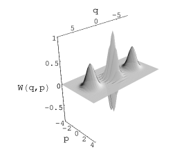
Figure 2: Wigner function $W(q,p)$ of a superposition of two Gaussian wave packets as in Fig. 1, here with $q_{1}=-5=-q_{2}$, $p_{1}=p_{2}=0$. The mutual distance is larger than individual spread. The oscillating pattern in between the two Gaussians indicates their coherence.

In terms of the Wigner function, (III.1) takes the form of a Fokker-Planck equation

$$\dot{W}_{t} = \left(-\frac{\partial}{\partial q}\frac{p}{M}+\frac{\partial}{\partial p}\left\{(M\Omega^{2}+a_{t})q+b_{t}p\right\}\right.$$ (19)

$$\left.+c_{t}\frac{\partial^{2}}{\partial p\partial q}+d_{t}\frac{\partial^{2}}{\partial p^{2}}\right)W_{t}\,.$$

We now read off the meaning of the coefficients $a,b,c,d$ in the evolution equations: while the term involving $a_{t}$ is a mere potential renormalization due to the coupling, the term involving $b_{t}$ describes damping. The two remaining terms represent diffusion; there is a mixed second-order derivative with coefficient $c_{t}$, while the time dependent momentum diffusion involving $d_{t}$ reflects the stochastic force of a classical Ohrnstein-Uhlenbeck type process. We remark that the first diffusion term turns out to be negligible in many cases. For a discussion of that latter as well as various other limits of physical relevance we refer the reader to masterosciref .

We may solve equation (19) with the help of the characteristic function or Fourier transform of the Wigner function,

$$\chi(\mu,\nu)=\frac{1}{2\pi\hbar}\int dqdp\;W(q,p){\rm e}^{{\rm i}(\mu q-\nu p)/\hbar}\,.$$ (20)

Interestingly, diffusive effects on $W$ can be confined to a Gaussian factor in $\chi$,

$$\chi_{t}(\mu,\nu) = \zeta_{t}(\mu,\nu)\exp(\int_{0}^{t}b(s)ds)$$

$$\times\exp\left(-\frac{1}{2\hbar^{2}}\left\{\alpha_{t}\mu^{2}+2\beta_{t}\mu\nu+\gamma_{t}\nu^{2}\right\}\right)\,;$$

the cofactor $\zeta$ then obeys the “Liouville” equation

$$\dot{\zeta}_{t}=\left(-\frac{\partial}{\partial\nu}\left(\mu/M+b_{t}\nu\right)+\frac{\partial}{\partial\mu}(M\Omega^{2}+a_{t})\nu\,\right){\zeta}_{t}\,,$$ (22)

provided the time dependent coefficients $\alpha,\beta,\gamma$ in the Gaussian (III.2) satisfy the linear equations

$$\left(\begin{array}[]{c}\dot{\alpha}_{t}\\ \dot{\beta}_{t}\\ \dot{\gamma}_{t}\end{array}\right)\! = \!\!\left(\!\begin{array}[]{ccc}0&-2/M&0\\ M\Omega^{2}+a_{t}&-b_{t}&-1/M\\ 0&2(M\Omega^{2}+a_{t})&-2b_{t}\end{array}\!\right)\left(\!\begin{array}[]{c}\alpha_{t}\\ \beta_{t}\\ \gamma_{t}\end{array}\!\right)$$ (36)

$$+\left(\begin{array}[]{c}0\\ -c_{t}\\ 2d_{t}\end{array}\right).$$

For the transformation to ensure $\zeta_{0}(\mu,\nu)=\chi_{0}(\mu,\nu)$, the initial condition for these coefficients is $(\alpha_{0},\beta_{0},\gamma_{0})=(0,0,0)$ at $t=0$.

We may solve the “Liouville equation” (22) through the characteristic equations

$${{\dot{\mu}}_{t}\choose{\dot{\nu}}_{t}}=\left({0\atop 1/M}{-(M\Omega^{2}+a_{t})\atop b_{t}}\right){\mu_{t}\choose\nu_{t}}$$ (37)

whose integral yields the linear mapping

$${\mu_{t}\choose\nu_{t}}=M_{t}{\mu_{0}\choose\nu_{0}}\,;$$ (38)

clearly, the $2\times 2$ matrix $M_{t}$ originates from the $2\times 2$ identity, $M_{0}={1\,0\choose 0\,1}$, at $t=0$. One can further establish the identity $\det M_{t}=\exp\left(\int_{0}^{t}b(s)ds\right)\,$ which will be useful below.

Given an arbitrary initial density operator and thus the corresponding initial characteristic function $\chi_{0}(\mu,\nu)$, we obtain the evolved $\chi_{t}(\mu,\nu)$ from (III.2), using

$$\zeta_{t}(\mu,\nu)=\int d\mu_{0}\int d\nu_{0}\chi_{0}(\mu_{0},\nu_{0})\delta(\mu-\mu_{t})\delta(\nu-\nu_{t}),$$ (39)

with $(\mu_{t},\nu_{t})$ the solutions (38) of the characteristic equations (37).

III.3 Coherence Norm for Distinct Wave Wackets

The Wigner function $W$ as well as its Fourier transform $\chi$ can be employed to express the norms $N_{ij}$ introduced in (7) and [SHB] as

$$N_{ij}(t) = (2\pi\hbar)\int dqdp\;|W^{ij}_{t}(q,p)|^{2}$$

$$= (2\pi\hbar)\int d\mu d\nu\;|\chi^{ij}_{t}(\mu,\nu)|^{2}\,.$$

The first of these expressions nicely shows that $N_{12}(t)$ is indeed a good indicator for the appearance of coherences between wave packets, as it measures the weight of the absolute square of the oscillating pattern of the Wigner function in between the wave packets as shown in Fig. 2. The second expression is most convenient to actually evaluate $N_{12}(t)$ for the oscillator model. In fact, the ansatz (III.2) and the general solution (39) yield

$$N_{12}(t) = (2\pi\hbar)\exp\{\int_{0}^{t}b(s)ds\}$$

$$\int\!d\mu_{0}d\nu_{0}{\rm e}^{-(\alpha_{t}\mu_{t}^{2}+2\beta_{t}\mu_{t}\nu_{t}+\gamma_{t}\nu_{t}^{2})/\hbar^{2}}|\chi^{12}_{0}(\mu_{0},\nu_{0})|^{2}$$

with $(\mu_{t},\nu_{t})$ the trajectories from (38).

With $\rho^{12}_{\rm sys}(0)=|\varphi_{1}\rangle\langle\varphi_{2}|$ and $|\varphi_{i}\rangle$ representing the Gaussian wave packets (5), simple Gaussian integrals give

$$|\chi_{0}^{12}(\mu_{0},\nu_{0})|^{2} = (2\pi\hbar)^{-2}\times$$

$$\exp\left\{-(\nu_{0}-d_{Q})^{2}/4\sigma-\sigma(\mu_{0}-d_{P})^{2}/\hbar^{2}\right\},$$

where $d_{Q}=|q_{2}-q_{1}|$ and $d_{P}=|p_{2}-p_{1}|$ denote the separations in position and momentum of the two wave packets. We thus see the characteristic function of the coherence to be strongly peaked near those distances, with both widths of order $\sqrt{\hbar}$ (Recall that we had chosen minimum uncertainty wave packets with $\sigma\sim\hbar$).

Evaluating the Gaussian integral in (III.3) results in the appealing form

$$N_{12}(t)={\cal P}(t)\exp\left\{-\frac{1}{\hbar^{2}}(d_{P},d_{Q})A_{t}{d_{P}\choose d_{Q}}\right\}$$ (43)

for the coherence norm, revealing the quadratic dependence of the decay on the initial separations $d_{Q},d_{P}$. The time dependence of this quadratic form is captured in the matrix $A_{t}$, which turns out bulky in this general case; it reads

$$A_{t}=C_{t}\left[\leavevmode\hbox{\small 1\kern-3.5pt\normalsize 1}+\left({1/\sigma\atop 0}{0\atop 4\sigma/\hbar^{2}}\right)C_{t}\right]^{-1}$$ (44)

with the matrix

$$C_{t}=M_{t}^{\rm T}\left({\alpha_{t}\atop\beta_{t}}{\beta_{t}\atop\gamma_{t}}\right)M_{t},$$ (45)

and $M_{t}$ the propagating matrix from (38). The functions $(\alpha_{t},\beta_{t},\gamma_{t})$ in (45) are the solutions of (36) with vanishing initial values (recall that the evolution of $(\alpha_{t},\beta_{t},\gamma_{t})$ involves the diffusion coefficients $c_{t}$ and $d_{t}$ while only the drift coefficients $a_{t}$ and $b_{t}$ enter the deterministic equation for $M_{t}$).

A prefactor

$${\cal P}(t)=\det\left(\leavevmode\hbox{\small 1\kern-3.5pt\normalsize 1}+\left({1/\sigma\atop 0}{0\atop 4\sigma/\hbar^{2}}\right)C_{t}\right)^{-\frac{1}{2}}\exp\{\int_{0}^{t}b(s)ds\}$$ (46)

appears in (43) which is independent of the separations and to be identified with the similar expression (3.14-SHB) in [SHB], resulting from the Gaussian integration. As explained in detail in [SHB], as long as the separation of the two wave packets is large compared to their individual spread, this ${\cal P}(t)$ may safely be replaced by unity for those short times for which $N_{12}$ decays to essentially zero due to the relevant exponential term in (43).

With the dependence of the coherence norm on the initial position and momentum separations $d_{Q},d_{P}$ now made explicit, we proceed to unveil the time dependence of the matrix $A_{t}$ in the exponent of the coherence norm (43), both for the interaction dominated early-time limit as well as for the long-time golden-rule limit. We stress again that due to the large separations $(d_{Q},d_{P})$ we focus on, the prefactor ${\cal P}(t)$ in (43) can and will be replaced by unity in what follows.

IV Limiting cases

IV.1 Golden Rule: $\tau_{\rm sys}\ll\tau_{\rm dec}\ll\tau_{\rm diss}$

Our exact result (43) for the coherence norm allows us to investigate the decay of coherences on all time scales. Matters simplify considerably in the case of weak coupling, where decoherence between the two wave packets may again be evaluated analytically.

Let us first determine the coefficients $(\alpha_{t},\beta_{t},\gamma_{t})$. To that end we first recall that these coefficients vanish initially and then realize that the inhomogeneities $c_{t},d_{t}$ are of second order in the interaction. We may therefore replace the $3\times 3$ propagator matrix in the evolution equation (36) in zeroth order, i.e. by entirely neglecting $a_{t}$ and $b_{t}$ therein. The propagator matrix is then easily exponentiated to give

$$\alpha_{t} = \int_{0}^{t}ds\;\Big{(}c(s)(\sin 2\Omega(t-s))/M\Omega$$

$$\;\;\;\;\;\;\;\;\;\;+d(s)(1-\cos 2\Omega(t-s))/M^{2}\Omega^{2}\Big{)},$$

$$\beta_{t} = -\int_{0}^{t}ds\;\Big{(}c(s)\cos 2\Omega(t-s)$$

$$\;\;\;\;\;\;\;\;\;\;+d(s)(\sin 2\Omega(t-s))/M\Omega\Big{)},$$

$$\gamma_{t} = -\int_{0}^{t}ds\;\Big{(}c(s)M\Omega\sin 2\Omega(t-s)$$

$$\;\;\;\;\;\;\;\;\;\;-d(s)(1+\cos 2\Omega(t-s))\Big{)}.$$

Moreover, we may replace the time dependent coefficients of the exact master equation (III.1) by their lowest-order expressions, which are

$$a_{t} = \int_{0}^{t}\!ds\,\langle\textstyle{\frac{{\rm i}}{\hbar}}[\tilde{B}(s),B]\rangle\cos\Omega s\;\;\;+{\cal O}(B^{4})$$ (48)

$$b_{t} = \frac{1}{M\Omega}\int_{0}^{t}\!ds\,\langle\textstyle{\frac{{\rm i}}{\hbar}}[\tilde{B}(s),B]\rangle\sin\Omega s\;\;\;+{\cal O}(B^{4})$$

$$c_{t} = \frac{1}{2M\Omega}\int_{0}^{t}\!ds\,\langle\{\tilde{B}(s),B\}\rangle\sin\Omega s\;\;\;+{\cal O}(B^{4})$$

$$d_{t} = \int_{0}^{t}\!ds\,\textstyle{\frac{1}{2}}\langle\{\tilde{B}(s),B\}\rangle\cos\Omega s\;\;\;+{\cal O}(B^{4}).$$

Note that perturbation theory preserves the correct short-time expansion (17).

Now that the coefficients $\alpha_{t},\beta_{t},\gamma_{t}$ within the matrix $C_{t}$ in (45) are revealed as of second order in the interaction, it suffices to replace $M_{t}$ by its zeroth-order approximant in that exponent. Neglecting the second-order terms $a_{t}$ and $b_{t}$ in the definition (38), we find

$$M_{t}=\left({\cos\Omega t\atop\sin\Omega t/M\Omega}{-M\Omega\sin\Omega t\atop\cos\Omega t}\right)\,.$$ (49)

With (IV.1) and (49) we have access to the full time dependence of the decohering quadratic form in the exponent of the coherence norm (43).

Of particular interest is the long-time limit, $\Omega t\gg 1$, which allows for many system oscillations up to the observation time. In that limit, furthermore assuming the bath correlation time to be much shorter than the system time scale $\Omega^{-1}$, we may safely replace the time dependent coefficients $c(s)$ and $d(s)$ by their asymptotic values $c(\infty)$, $d(\infty)$ under the integrals in (IV.1). Moreover, we see from the latter expressions that for $\Omega t\gg 1$ all oscillating terms vanish and the only surviving contribution arises from the constant terms involving $d(\infty)$. The Golden-Rule limit $\Omega t\gg 1$ thus finally yields the coefficients

$$\alpha_{t} = \frac{d(\infty)}{M^{2}\Omega^{2}}t,$$ (50)

$$\beta_{t} = 0,$$

$$\gamma_{t} = d(\infty)t$$

and the matrix (45)

$$C_{t}=d(\infty)t\left({\frac{1}{M^{2}\Omega^{2}}\atop 0}{0\atop 1}\right)\,.$$ (51)

With $C_{t}$ already of second order in the in the interaction, we see from (44) that $A_{t}$ coincides with $C_{t}$ in this order of perturbation theory. The well known exponential decay

$$N_{12}(t)=\exp\left\{-\frac{d(\infty)t}{\hbar^{2}}\Big{(}d_{Q}^{2}+d_{P}^{2}/M^{2}\Omega^{2}\Big{)}\right\}\equiv{\rm e}^{-t/\tau_{\rm dec}^{\rm GR}}$$ (52)

characteristic of golden-rule decoherence results (recall that we may drop the slowly varying prefactor ${\cal P}(t)$ of the general expression (43)). Clearly, since we allow the system to evolve for many cycles, any distinction of the position as the coupling agent in the interaction Hamiltonian has disappeared. Through the sequence of system cycles, position and momentum interchange their role periodically such that in the long-time limit of decoherence only the joint quantity $\left((d_{Q})^{2}+(d_{P})^{2}/(M^{2}\Omega^{2})\right)$ appears as acceleration factor.

For the final result for the golden-rule decoherence time we still have to determine the rate $d(\infty)$. In the relevant order of perturbation theory and upon using the bath correlation function (III,12) we get

$$d(\infty) = \int_{0}^{\infty}\!ds\;\textstyle{\frac{1}{2}}\langle\{\tilde{B}(s),B\}\rangle\cos\Omega s$$ (53)

$$= \hbar M\gamma\Omega f_{c}(\Omega/\Lambda)(n_{\rm th}+\textstyle{\frac{1}{2}})\,;$$

where again $n_{\rm th}=({\rm e}^{\hbar\Omega/kT}-1)^{-1}$ is the thermal number of quanta in the oscillator and $f_{c}(\Omega/\Lambda)\to 1$ according to (13) . Comparing with the lowest-order drift coefficient

$$b(\infty) = \frac{1}{M\Omega}\int_{0}^{\infty}\!ds\frac{{\rm i}}{\hbar}\langle[\tilde{B}(s),B]\rangle\sin\Omega s$$ (54)

$$= \gamma f_{c}(\Omega/\Lambda)\to\gamma$$

we recover the previously announced interpretation of $\gamma$ as the classical damping constant, $\gamma=1/\tau_{\rm diss}$, as well as the well known golden-rule decoherence time $\tau_{\rm dec}^{\rm GR}$ already presented in (1.2-SHB) of [SHB]. That latter expression implies the familiar golden-rule time-scale ratio for decoherence and dissipation,

$$\frac{\tau_{\rm dec}^{\rm GR}}{\tau_{\rm diss}^{\rm GR}}=\left(\frac{\lambda_{\rm th}}{d_{\rm eff}}\right)^{2}\,;$$ (55)

we see decoherence accelerated over dissipation by the squared ratio of a de Broglie wavelength $\lambda_{\rm th}=\sqrt{\hbar/M\Omega(n_{\rm th}+1/2)}$ and an effective distance between the two wave packets, $d_{\rm eff}=\sqrt{d_{Q}^{2}+d_{P}^{2}/M^{2}\Omega^{2}}$.

IV.2 Interaction dominance 1: $\tau_{\rm dec}\ll\tau_{\rm sys},\tau_{\rm diss}$

As soon as the initial separation $(d_{Q},d_{P})$ between wave packets extends beyond quantum scales, decoherence is dominated by the interaction Hamiltonian $H_{\rm int}$ since the free motion generated by $H_{\rm sys}$ eventually becomes negligibly slow by comparison. This is the regime we discussed at length and in a general setting in the accompanying paper [SHB]. We must recover those previous findings for the exactly solvable oscillator model by suitably simplifying the general expression (43) for the coherence norm.

During these very short initial time spans, we take into account dynamics on classical time scales due to the “Liouville equation” (22) to lowest order in $t$ only and replace the corresponding propagating matrix $M_{t}$ in (38) by $M_{t}=\left({1\atop t/M}{-M\Omega^{2}t\atop 1}\right)+{\cal O}(t^{2})$. Next, we have to determine the coefficients $\alpha_{t},\beta_{t}$ and $\gamma_{t}$ in (36). As before, we expand all dynamical quantities connected to the oscillator dynamics to the lowest relevant order in $t$ and find

$$\alpha_{t} = \int_{0}^{t}ds\;\textstyle{\langle\frac{1}{2}}\{\tilde{B}(s),B(0)\}\rangle(2t+s)(t-s)^{2}/3M^{2},$$

$$\beta_{t} = -\int_{0}^{t}ds\;\langle\textstyle{\frac{1}{2}}\{\tilde{B}(s),B(0)\}\rangle t(t-s)/M,$$

$$\gamma_{t} = -\int_{0}^{t}ds\;\langle\{\tilde{B}(s),B(0)\}\rangle.$$ (56)

We see the importance of the details of the (real part of the) bath correlation function, $\langle\frac{1}{2}\{\tilde{B}(s),B(0)\}\rangle$, describing dynamics on reservoir time scales.

The matrix (45) determining the decay of coherences is

$$C_{t}=\int_{0}^{t}ds\; \langle\textstyle{\frac{1}{2}}\{\tilde{B}(s),B(0)\}\rangle(t-s)$$

$$\times\left({(t-s)(2t+s)/3M\atop t/M}\;\;\;{t/M\atop 2}\right)\,.$$

As in the weak coupling case, the difference between the relevant matrix $A_{t}$ in (44) and $C_{t}$ is negligible for the fast decoherence resulting from large separations $(d_{Q},d_{P})$, and with $A_{t}$ replaced by (IV.2), we get from (43) the coherence norm as the exponential

$$N_{12}(t) = \exp\,\Bigl{\{}-\frac{1}{\hbar^{2}}\int_{0}^{t}ds\;\langle\{\tilde{B}(s),B(0)\}\rangle(t-s)$$

$$\times\left({d_{Q}}^{2}+d_{Q}d_{P}t/M+{d_{P}}^{2}(t-s)(2t+s)/6M^{2}\right)\Bigr{\}},$$

see BHS and [SHB] for the case $d_{P}=0$. As before, we may neglect the slowly varying prefactor ${\cal P}(t)$ of the exact expression (43).

Two remarks about this expression are in order. First, the oscillator model clearly confirms the general result (6.5-SHB) (for $d_{P}=0$) of the accompanying paper [SHB], that derivation being based solely on the assumption $\tau_{\rm dec}\ll\tau_{\rm sys},\tau_{\rm diss}$ and the Gaussian character of the bath coupling agent. Secondly, (IV.2) may be recognized to coincide with the squared absolute norm of the Feynman-Vernon influence functional feynman ; feynman2 , with the classical paths represented by the short-time expression $q_{t}=q_{1}+p_{1}t/M$ (replace one by two for the second path $q^{\prime}_{t}$). Examples of decoherence following (IV.2) will be shown in Sect. VI.

IV.3 Interaction dominance 2: $\tau_{\rm dec}\ll\tau_{\rm res},\tau_{\rm sys},\tau_{\rm diss}$

In the extreme case when decoherence is even faster than any environmental time scale it is sufficient to expand the whole matrix $A_{t}$ in the exponent of (43) in powers of the elapsed time $t$, mirroring the corresponding expansion of the logarithm of the interaction propagator in [SHB]. Crucially, we replace the correlation function $\frac{1}{2}\langle\{\tilde{B}(s),B(0)\}\rangle$ under the integral by its initial value $\langle B^{2}\rangle$. Starting from (IV.2) of the last section we find

$$C_{t}=\langle B^{2}\rangle\left({\frac{t^{4}}{4M^{2}}\atop\frac{t^{3}}{2M}}{\frac{t^{3}}{2M}\atop t^{2}}\right),$$ (59)

in each entry neglecting higher order terms. Again, the short time approximation demands $A_{t}$ to be identical to $B_{t}$ from (59) to the relevant order, and the general result (43) turns into

$$N_{12}(t) = \exp\left\{-\frac{1}{\hbar^{2}}\langle B^{2}\rangle\right.$$

$$\left.\left({d_{Q}}^{2}t^{2}+d_{Q}d_{P}t^{3}/M+{d_{P}}^{2}t^{4}/4M^{2}\right)\right\}$$

which is the universal law (3.14-SHB) for the decay of coherences we found under very general conditions in the accompanying paper [SHB] and for $d_{P}=0$ in BHS . We refrain from including the prefactor ${\cal P}(t)$ here, that factor in (3.14-SHB) being safely replaced by unity for the relevant short times characteristic of the decay for asymptotically classical initial separations $d_{Q}$, $d_{P}$.

Any coherences present in the system will have vanished according to (IV.3), before the quantum state can be aware of any potential $V(Q)$ – this is why the oscillator frequency $\Omega$ has disappeared entirely from the final expression (IV.3) (and also from (IV.2)). Recall that system oscillations with frequency $\Omega$ were crucial for the golden-rule result. Eq. (IV.3) also confirms the different scalings of the corresponding decoherence times $\tau_{\rm dec}^{Q}$, $\tau_{\rm dec}^{QP}$, and $\tau_{\rm dec}^{P}$ discussed in great detail in the fourth section of [SHB].

V An alternative measure for decoherence

Before turning to actual examples, we replace the general coherence norm $N_{12}(t)$ by a somewhat simpler quantity with equal power to reveal decoherence.

As we are going to restrict ourselves to superpositions of symmetrically located wave packets with $q_{2}=-q_{1}$, and $p_{2}=-p_{1}$, an alternative indicator of the decay of coherences is the value of the Wigner function of $\rho_{\rm sys}$ at the origin,

$$W_{t}(0,0)=\frac{1}{\pi\hbar}\int dq\langle q|\rho|-q\rangle=\frac{1}{\pi\hbar}\int dp\langle p|\rho|-p\rangle.$$ (61)

Apparently, $W_{t}(0,0)$ is a measure for the weight off the diagonal, both in the position and momentum representations; it is linear in the density operator and hence easier to access numerically, given the master equation; it is intimately related to the previously employed $N_{12}(t)$ as we will briefly show. By definition, we have $W_{t}(0,0)=\frac{1}{2\pi\hbar}\int d\mu d\nu\chi_{t}(\mu,\nu)=\frac{1}{2\pi\hbar}\int d\mu d\nu\sum_{ij}c_{i}c_{j}^{*}\chi_{t}^{ij}(\mu,\nu)$. The diagonal terms $\chi_{t}^{11}$ and $\chi_{t}^{22}$ do not noticeably contribute to $W_{t}(0,0)$ since for superpositions of far-apart wave packets their Wigner correspondant is located near $(q_{1},p_{1})$, and $(-q_{1},-p_{1})$, respectively, i.e. far away from the phase space origin, as is also apparent in Fig. 2. Furthermore, for the symmetric case considered here, we find real Gaussians for the characteristic functions such that $\chi_{t}^{12}=\chi_{t}^{21}=|\chi_{t}^{21}|$ and therefore

$$W_{t}(0,0)\propto\int d\mu d\nu|\chi_{t}^{12}(\mu,\nu)|\,.$$ (62)

Comparing the latter with expression (III.3) for the norms $N_{ij}$ we see that for the symmetric superposition of wave packets considered here, the linear quantity $W_{t}(0,0)$ has equal power to reveal the fate of coherence as the coherence norm $N_{12}(t)$. Going through the very same steps as in the previous section we find

$$n_{12}(t) \equiv W_{t}(0,0)/W_{0}(0,0)$$

$$= {\cal P}(t)\exp\left\{-\frac{1}{2\hbar^{2}}(d_{P},d_{Q})A_{t}{d_{P}\choose d_{Q}}\right\}\,,$$

with the same prefactor ${\cal P}(t)$ and matrix $A_{t}$ as in the expression (43) for $N_{12}(t)$. Neglecting the irrelevant prefactor ${\cal P}(t)$ reveals that the simpler quantity $n_{12}(t)$ is essentially just the square root of the coherence norm $N_{12}(t)$ and our previous discussion of that quantity in Sect. III equally applies to $n_{12}(t)$.

VI Numerical results for the Oscillator model

We illustrate numerically the decoherence of a superposition of two symmetrically located coherent states, $|\varphi_{1}\rangle=|\alpha\rangle$ and $\varphi_{2}=|-\alpha\rangle$, which are labeled by a complex number $\alpha$, $|\alpha\rangle={\rm e}^{-\frac{1}{2}|\alpha|^{2}}{\rm e}^{\alpha a^{+}}|0\rangle$, see Glauber . The dimensionless creation and annihilation operators, for instance $a=\left(\sqrt{M\Omega/2\hbar}\;Q+{\rm i}P/\sqrt{2M\Omega\hbar}\right)$, contain the quantum reference scales of length and momentum characteristic of the harmonic oscillator. We may employ those scales to introduce dimensionless distances between the two coherent states

$${\tilde{d}}_{Q} = d_{Q}/\sqrt{\hbar/M\Omega}=\sqrt{2}(\alpha+\alpha^{*})$$ (64)

$${\tilde{d}}_{P} = d_{P}/\sqrt{M\hbar\Omega}=\sqrt{2}(\alpha-\alpha^{*})/{\rm i}\,,$$

which will be the relevant quantities in the following. In these units, large separations with respect to the spread of coherent states, as required for our general formula (43), simply means large compared to unity. Truly macroscopic separations could lead to dimensionless separations of the order, say, ${\tilde{d}}_{Q}\simeq 10^{17}$, a scale way beyond our examples below. We shall let ${\tilde{d}}_{Q}$ or ${\tilde{d}}_{P}$ range from $16$ to $4000$ and in one extreme case to $800000$. It will become clear that the transition from slow golden-rule decoherence to rapid interaction dominated decoherence is fully captured in the mesoscopic range considered.

We assume a thermal environment with all parameters of the total Hamiltonian fixed once and for all. It is the initial state of the system oscillator only that we alter between simulations. The transition we are after is traced out by varying the dimensionless initial phase space distances $({\tilde{d}}_{Q},{\tilde{d}}_{P})$ between the superposed wave packets.

All simulations are performed with the small damping rate $\gamma=10^{-5}\Omega$, a rather large temperature according to $k_{B}T=20\hbar\Omega$, and an environmental cutoff frequency $\Lambda=100\Omega$. The latter is the largest frequency involved in either system or environment. We expect interaction dominated decoherence according to (IV.2) to set in as soon as the decoherence time scale becomes shorter than the shortest system time scale, here $\Omega^{-1}$. The extreme case of quadratic decay according to (IV.3) (or qubic or quartic, depending on the nature of the superposition - see also [SHB]) occurs as soon as $\tau_{\rm dec}$ is even shorter than reservoir time scales, here determined by $\Lambda^{-1}$. The numerical solution of the exact master equation is based on the corresponding exact stochastic Schrödinger equation for this model, as established recently Stochastic . This approach has the nice feature of preserving Gaussian pure states within each run of the Schrödinger equation for a given realization of the driving noise and, moreover, allows easy access to the otherwise involved expressions for the time dependent coefficients entering the evolution equations.

VI.1 Golden rule

We can estimate for which dimensionless effective separation ${\tilde{d}}_{\rm eff}=\sqrt{{\tilde{d}}_{Q}^{2}+{\tilde{d}}_{P}^{2}}$ the golden rule result should apply for our choice of parameters. ¿From (52) and (53) we find $\tau_{\rm dec}^{\rm GR}=\left(\gamma(n_{\rm th}+1/2){\tilde{d}}_{\rm eff}^{2}\right)^{-1}$. Recall that the golden rule assumes a long-time limit $\Omega t\gg 1$. We can thus trust the golden rule decay law only as long as $\Omega\tau_{\rm dec}^{\rm GR}\gg 1$ which puts an upper bound on ${\tilde{d}}_{\rm eff}$. Together with the lower bound arising from the requirement of a large separation we have

$$1\ll{\tilde{d}}_{\rm eff}\ll\sqrt{\Omega/\gamma(n_{\rm th}+1/2)}\,.$$ (65)

For the choice of parameters above, we find $1\ll{\tilde{d}}_{\rm eff}\ll 70$, a fairly narrow band for the applicability of the golden rule.

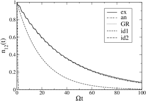
Figure 3: Golden-rule decay of an initial superposition of two coherent states. Distances are ${\tilde{d}}_{Q}=16$ and ${\tilde{d}}_{P}=0$. Environmental parameters are $\gamma=10^{-5}\Omega$, $\Lambda=100\Omega$, and $kT=20\hbar\Omega$. Full line (“ex”): exact numerical calculation, indistinguishable from the analytical expression (43) (dash-dotted, “an”). Dotted line (“GR”): golden-rule result (52) which fits smoothly through the slightly oscillatory exact result. Interaction-dominance results (dashed lines, “id1”, “id2”) are irrelevant here; the influence of the system Hamiltonian is crucial.

In Fig. 3 we show the decay of an initial superposition of two coherent states with separations ${\tilde{d}}_{\rm eff}={\tilde{d}}_{Q}=16$ and thus ${\tilde{d}}_{P}=0$. The full line (“ex”) shows the exact numerical result. Apart from some tiny oscillations around the exponential decay the golden-rule expectation (dotted and labeled “GR”) according to (52) is nicely confirmed. Note how the tiny oscillations loose final relevance as soon as $\Omega t\gg 1$. These oscillations have their origin in the periodic change of the system state between a superposition with respect to $Q$ to one with respect to $P$. Decoherence is more efficient for $Q$-superpositions, and less effective in those time spans when the system state assumes a superposition with respect to $P$. During those periods decoherence is slowed down slightly. During one oscillator period there are two swaps between a $Q$- and a $P$-superposition, which fact explains the frequency $2\Omega$ of the oscillations in question. The dash-dotted line (“an”) depicts the analytical expression (43) and is almost indistinguishable from the exact result. The two dashed curves (“id1”, “id2”) correspond to predictions from the two interaction dominated regimes. They are clearly irrelevant for the still “slow” decoherence of the underlying “microscopic” superposition. The system Hamiltonian has a strong influence on the decay in that regime.

VI.2 Crossover regime: $\tau_{\rm dec}\approx\tau_{\rm sys}$

The golden rule ceases to be relevant as soon as the initial separation between the superposed wave packets increases to such an extent that the decoherence time scale $\tau_{\rm dec}$ becomes comparable to $\tau_{\rm sys}$. Then the decay must still be system specific, that is depend on the details of the dynamics induced by the system Hamiltonian and the time scales emerging from the bath correlation function. It is the special virtue of the oscillator model to allow rigorous treatment of this crossover case.

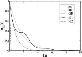
Figure 4: Crossover regime, ${\tilde{d}}_{Q}=80$ and ${\tilde{d}}_{P}=0$, otherwise same parameters as in Fig. 3. Golden rule no longer valid, universal interaction dominated regime not yet reached. Full line (“ex”)for exact numerical calculation; indistinguishable dash-dotted line (“an”) for (43). Only for small times, $\Omega t\ll 1$, decay according to (IV.2) (“id1”) becomes visible. Oscillations due to system Hamiltonian, see main text.

Fig. 4 shows the decay of an initial superposition of coherent states with an intermediate position separation ${\tilde{d}}_{Q}=80$ and equal momenta, ${\tilde{d}}_{P}=0$. The (indistinguishable) full and dash-dotted lines show the exact master equation result and the evaluation of the exact analytical expression (43). We see that decoherence due to coupling to the position is very effective initially; however, as the system dynamics moves the $Q$-superposition to one with respect to $P$ after a quarter of the oscillator period $\Omega t\approx\pi/2$, decoherence slows down. Turning the state further in phase space, decoherence becomes efficient again after another quarter of the period, and periodically thereafter. The periodic alteration between slowdown and acceleration is now a prominent feature rather than a small fluctuation. For times short compared to the system time scale, $\Omega t\ll 1$, the influence of the system Hamiltonian is negligible and thus the general result (IV.2) of interaction dominance (dashed line, “id1”) initially applies as can be seen from the good agreement for short times.

VI.3 Interaction dominated decoherence 1

As soon as the separations ${\tilde{d}}_{Q}$ or ${\tilde{d}}_{P}$ between the superposed coherent states are sufficiently large, the system Hamiltonian becomes irrelevant and interaction dominates, see Fig. 5. For a separation of ${\tilde{d}}_{Q}=200$ and equal momenta ${\tilde{d}}_{P}=0$, decoherence is faster than any system time scale, yet still longer than the environmental correlation time $\Lambda^{-1}$. This is the regime that can fully be described by the general decay law (6.5-[SHB]) of the accompanying paper [SHB], here (IV.2). As mentioned in [SHB], unless the spectral density differs from zero at zero frequency – which is not the case here, (IV.2) describes non-exponential decay. We further remark that the golden rule (dotted line, “GR”) now predicts far too slow decoherence.

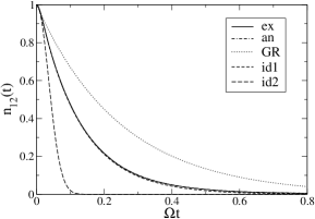
Figure 5: Interaction dominance, ${\tilde{d}}_{Q}=200$ and ${\tilde{d}}_{P}=0$, otherwise same as in Fig. 3; note change of time scale. Full line (“ex”) for exact numerical calculation, indistinguishable dash-dotted line (“an”) for (43). Golden rule (dotted line, “GR”) now meaningless; interaction dominance (dashed line, “id1”) throughout whole relevant time span. Extreme short-time result (IV.3) (dashed line, “id2”) enters validity for very early times.

VI.4 Interaction dominated decoherence 2

We expect universal decay according to our simple analytical expression (IV.3) (corresponding to result (3.14-[SHB]) in [SHB]) as soon as the decoherence time is the shortest time scale involved, here even shorter than the inverse environmental cutoff frequency $\Lambda^{-1}$. We thus find lower bounds for the size of superpositions that indicate the beginning of this universal interaction dominated decoherence regime.

We use (14) to find an expression for $\langle B^{2}\rangle$ and conclude from the discussion of interaction dominated decoherence times in [SHB] that for a superposition in position space, $\Lambda\tau_{\rm dec}^{Q}\simeq\sqrt{\hbar\Lambda\Omega/(kT\gamma)}/{\tilde{d}}_{Q}$. The latter has to be small compared to one in order for this universal regime to be important. With the choice of parameters as before, we find the condition ${\tilde{d}}_{Q}\gg 700$ for the universal Gaussian decay law to be relevant.

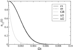
Figure 6: Interaction dominated universal decoherence, ${\tilde{d}}_{Q}=4000$ and ${\tilde{d}}_{P}=0$, otherwise as in Fig. 3; note change of time scale. Four results in agreement: full line (“ex”) for exact numerical calculation, dash-dotted line (“an”) for analytical formula (43), two dashed lines (“id1” and “id2”) for interaction dominance, the latter the Gaussian $\exp\{-(t/\tau_{\rm dec}^{Q})^{2}\}$ from (IV.3). Golden rule (dotted line, “GR”) grossly underestimates life time of coherence.

In Fig. 6 we show the decay of an initial superposition of coherent states with a yet larger separation ${\tilde{d}}_{Q}=4000$ and ${\tilde{d}}_{P}=0$. Note the difference in time scales along the $t$-axis between the various figures. While the full line (“ex”) represents the exact numerical calculation, the dash-dotted line (“an”) is our exact formula (43). In this case, interaction dominance holds (dashed lines, “id1” and “id2”), the extreme short-time result (IV.3) suffices to describe the decay over the full relevant time interval. The latter is a Gaussian $\exp\{-(t/\tau_{\rm dec}^{Q})^{2}\}$ decay law. Clearly, the golden rule is not applicable here and wrongly predicts far too fast decoherence. This is due to the quadratic golden rule scaling of the decoherence times with distance, as compared to only a linear dependence of the true interaction dominated decoherence time [SHB].

A superposition in momentum space with equal positions ${\tilde{d}}_{Q}=0$ is more stable under the position dependent coupling $H_{\rm int}=QB$ between system and environment. To reveal interaction dominance and our universal decay law, a momentum superposition will have to be much larger (in our dimensionless units) than a position space superposition. As in the previous case, we get an estimate for the border of applicability of our universal law (see the discussion in the accompanying paper [SHB]) $\Lambda\tau_{\rm dec}^{P}\simeq\left(\hbar\Lambda^{3}/(kT\Omega\gamma)\right)^{\frac{1}{4}}/\sqrt{{\tilde{d}}_{P}}$. This quantity has to be small compared to one for universal “quartic” decay. For our choice of parameters, ${\tilde{d}}_{P}\gg 70000$ is required.

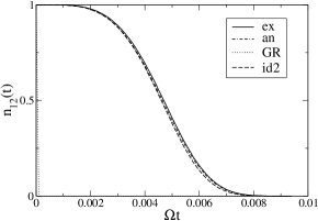
Figure 7: Interaction dominated universal decay of initial superposition of two coherent states with opposite momenta and equal positions. Distances are ${\tilde{d}}_{Q}=0$ and ${\tilde{d}}_{P}=800000$, other parameters as in Fig. 3; note change of time scale. Four results in agreement: full line (“ex”) for exact numerical calculation, dash-dotted line (“an”) for analytical formula (43), and a dashed line (“id2”) of interaction dominance, the latter now the quartic exponential $\exp\{-(t/\tau_{\rm dec}^{P})^{4}\}$ law (IV.3). Golden rule (dotted line “GR”) underestimates lifetime of coherence even more drastically as in Fig. 6.

We check on that case in Fig. 7 which depicts the decay of an initial superposition of two coherent states with momentum separation ${\tilde{d}}_{P}=800000$ and equal positions ${\tilde{d}}_{Q}=0$. As before, the full line (“ex”) is the exact numerical result compared with (43) (dash-dotted line) and the interaction dominated results (dashed line, “id2”). Again, the golden rule by far underestimates the decoherence time, due to the wrong scaling: while $\tau_{\rm dec}^{GR}$ scales with ${\tilde{d}}_{P}^{2}$, the true $\tau_{\rm dec}^{P}$, as it may be determined from our approach to interaction dominated decoherence [SHB], scales with the square root $\sqrt{{\tilde{d}}_{P}}$ only. However, Fig. 7 does confirm the quartic decay $n_{12}(t)=\exp\{-(t/\tau_{\rm dec}^{P})^{4}\}$ we predict according to (IV.3).

VII Conclusions

The exactly soluble model of a damped harmonic oscillator coupled to bath of oscillators illustrates our prediction of various decoherence scenarios. For microscopic distances between the superposed wave packets, decoherence is so slow as to witness many free-system cycles and follows the standard exponential golden-rule decay. As the separation increases, decoherence and system time scales eventually become comparable and a more complicated, system-specific decay of coherences results. Our findings indicate that golden-rule predictions may fail for even only moderately sized superpositions. For further increased separations we enter interaction dominated decoherence as presented in BHS and in much more detail in the accompanying paper [SHB]. Now $\tau_{\rm dec}\ll\tau_{\rm sys}$ and decoherence proceeds according to a system-independent decay law (IV.2), incorporating the bath correlation function. In the extreme case when decoherence even outruns intra-bath processes, the decay becomes a simple Gaussian for an initial separation with respect to position, and an initially slower fourth-order exponential if momentum is the differing property; position is distinguished over momentum since it is taken as the system coupling agent in the interaction with the bath.

The special virtue of the oscillator model studied here is to allow inspection of the crossover between the long-time golden rule regime valid for microscopic superpositions, and the interaction dominated regime relevant for more and more macroscopic superpositions.

As experimental efforts towards resolving decoherence dynamics continue experiments , it will be fascinating to see whether larger-scale superpositions can be realized and whether decoherence dynamics can be pushed towards the interaction dominated regime illustrated here and in [SHB].

References

- (1) W. T. Strunz, F. Haake, and D. Braun, Phys. Rev. A. (accompanying paper).
- (2) J. R. Senitzky, Phys. Rev. 119, 670 (1960); F. Schwabl, W. Thirring, Ergeb. exakt. Naturwiss. 36, 219 (1964); G. W. Ford, M. Kac, and P. Mazur, J. Math. Phys. 6, 504 (1965); P. Ullersma, Physica 32, 27 (1966); A.O. Caldeira, A.J. Leggett, Phys. Rev. A31, 1059 (1985); F. Haake, M. Żukowski, ibid. A47, 2506 (1993).
- (3) F. Haake, R. Reibold, Phys. Rev. A32, 2462 (1985); B. L. Hu, J. P. Paz, and Y. Zhang, Phys. Rev. D45, 2843 (1992).
- (4) D. Giulini, E. Joos, C. Kiefer, J. Kupsch, I.O. Stamatescu, H.D. Zeh, Decoherence and the appearance of a classical world in quantum theory (Springer, Berlin 1996).
- (5) W.H. Zurek, Phys. Today 44, 36-44 (1991); W.H. Zurek, S. Habib, J.P. Paz, Phys. Rev. Lett. 70, 1187 (1993); J.P. Paz, W.H. Zurek, Phys. Rev. Lett. 82, 5181 (1999)
- (6) J. P. Paz, S. Habib, W. H. Zurek, Phys. Rev. D47, 488 (1993).
- (7) R.J. Glauber, Phys. Rev. 131 2766 (1963); C.G. Sudarshan, Phys. Rev. Lett. 10, 277 (1963).
- (8) R.P. Feynman, F.L. Vernon, Ann. Phys. (N.Y.) 24, 118 (1963).
- (9) W. G. Unruh and W. H. Zurek, Phys. Rev. D40, 1071 (1989); G. W. Ford and R. F. O’Connell, Phys. Rev. D64, 105020 (2001).
- (10) U. Weiss, Quantum dissipative systems, (World Scientfic, Singapore), 2nd edition, (2000).
- (11) To save a little space we shall in the sequel mostly write the time argument as an index and even sometimes drop the latter.
- (12) D. Braun, F. Haake, and W. T. Strunz, Phys. Rev. Lett. 86, 2913 (2001).
- (13) We thank D. Cohen for drawing our attention to this connection.
- (14) L. Diosi, N. Gisin, and W. T. Strunz, Phys. Rev A58, 1699 (1998); W. T. Strunz, Chem. Phys. 268 237 (2001).
- (15) M. Brune, Phys. Rev. Lett. 77, 4887 (1996); C.J. Myatt, B.E. King, Q.A. Turchette, C.A. Sackett, D. Kielpinski, W.M. Itano, C. Monroe, D.J. Wineland, Nature 403, 269 (2000).