High-Order Variational Perturbation Theory for the Free Energy

Abstract

In this paper we introduce a generalization to the algebraic Bender-Wu recursion relation for the eigenvalues and the eigenfunctions of the anharmonic oscillator. We extend this well known formalism to the time-dependent quantum statistical Schrödinger equation, thus obtaining the imaginary-time evolution amplitude by solving a recursive set of ordinary differential equations. This approach enables us to evaluate global and local quantum statistical quantities of the anharmonic oscillator to much higher orders than by evaluating Feynman diagrams. We probe our perturbative results by deriving a perturbative expression for the free energy which is then subject to variational perturbation theory as developed by Kleinert, yielding convergent results for the free energy for all values of the coupling strength.

I Introduction

Most physical problems can only be solved by approximation methods. One of them is perturbation theory which yields weak-coupling expansions. Unfortunately, they often do not converge.
The ground state energy of the anharmonic oscillator is the simplest example where this phenomenon can be studied. Algebraic recursion relations à la Bender and Wu Bender/Wu yield perturbation series for the eigenvalues (energy) and eigenfunctions (wave functions) of the time-independent Schrödinger equation up to arbitrarily high orders. In Ref. exp the calculation was extended to 250th order. The Bender-Wu recursion relation yields a power series for the anharmonic part of the wave function both in the coupling strength $g$ and in the coordinate $x$. The power series in $x$ can be cut off naturally by comparing the recursive results with those obtained from evaluating Feynman diagrams. The resulting weak-coupling series for the ground state energy does not converge for any value of the coupling strength. This paper deals with both problems: Obtaining high-order perturbation expressions and making them converge for all values of the coupling strength. It is organized as follows:
In Sec. II we perturbatively evaluate the path integral representation for the imaginary-time evolution amplitude of the anharmonic oscillator by means of a generalized Wick’s theorem weissbach ; bachmann . In Sec. III we represent the first-order results diagrammatically. Doing so, we demonstrate that the algebraic computational cost is very high for the diagrammatic approach. We also obtain a cross check for the results which are derived from a differential recursion relation in the subsequent Sec. IV. In order to cut down on the algebraic computational cost we introduce a strategy to exploit the symmetry property of the imaginary-time evolution amplitude in Sec. V, thus laying the foundation for our high-order results. In Sec. VI we combine the resulting algebraic recursion relation with the original differential recursion relation, thus generalizing the Bender-Wu approach Bender/Wu . From our perturbative results for the imaginary-time evolution amplitude we then gain a perturbation expression for the free energy of the anharmonic oscillator in Sec. VII which we check again diagrammatically in Sec. VIII. The perturbative results are then re-summed in Sec. IX by means of variational perturbation theory Kleinert for intermediate coupling $g=1$ for which the usual weak-coupling series would diverge. This theory is a systematic extension of a simple variational approach, first developed by Feynman and Kleinert in the path integral formalism. Feynman introduced the path integral formalism as a quantization regulation, that represents the operator properties of quantum physics by fluctuations of the dynamical variables Feynman1 ; Feynmanhibbs . By extending analytically real time to imaginary time, also quantum statistical quantities can be obtained by summing over quantum mechanical and thermal fluctuations with the help of path integrals Feynmanhibbs ; Feynman2 . In order to evaluate the path integral for the free energy approximatively, Feynman and Kleinert developed a variational method in 1986 Feynman . It replaces the relevant system by the exactly solvable harmonic oscillator whose frequency becomes a variational parameter which has to be optimized. Starting with Ref. Kleinert2 , this method has been systematically extended by Kleinert to higher orders Kleinert ; Frohlinde . It is now known as variational perturbation theory and yields results for all temperatures and all coupling strengths.
In Sec. X we extend this procedure to higher orders of the free energy and cross check the results in Sec. XI.

II Path Integral Representation

The path integral representation for the imaginary-time evolution amplitude of a particle of mass $M$ moving in a one dimensional potential $V(x)$ reads Kleinert

$$(x_{b}\,\hbar\beta|x_{a}\,0) = \int_{x(0)=x_{a}}^{x(\hbar\beta)=x_{b}}{\cal D}x\exp\left\{-\frac{1}{\hbar}\int_{0}^{\hbar\beta}d\tau\right.$$ (1)

$$\left.\left[\frac{M}{2}\dot{x}^{2}(\tau)+V(x(\tau))\right]\right\}\,.$$

For the anharmonic oscillator potential

$$V(x)=\frac{M}{2}\omega^{2}x^{2}+gx^{4}$$ (2)

the imaginary-time evolution amplitude (1) can be expanded in powers of the coupling constant $g$. Thus we obtain the perturbation series

$$(x_{b}\,\hbar\beta|x_{a}\,0)=(x_{b}\,\hbar\beta|x_{a}\,0)_{\omega}$$

$$\times\left[1-\frac{g}{\hbar}\int_{0}^{\hbar\beta}d\tau_{1}\langle x^{4}(\tau_{1})\rangle_{\omega}+\,...\right]\,,$$

where we have introduced the harmonic imaginary-time evolution amplitude

$$(x_{b}\,\hbar\beta|x_{a}\,0)_{\omega}\equiv\int_{x(0)=x_{a}}^{x(\hbar\beta)=x_{b}}{\cal D}x$$

$$\times\exp\Bigg{\{}-\frac{1}{\hbar}\int_{0}^{\hbar\beta}d\tau\left[\frac{M}{2}\dot{x}^{2}(\tau)+\frac{M}{2}\omega^{2}x^{2}(\tau)\right]\Bigg{\}}\,,$$

and the harmonic path expectation value for an arbitrary functional $F[x]$:

$$\langle F[x]\rangle_{\omega}\equiv\frac{1}{(x_{b}\,\hbar\beta|x_{a}\,0)_{\omega}}\int_{x(0)=x_{a}}^{x(\hbar\beta)=x_{b}}{\cal D}x\,F[x]$$

$$\times\exp\left\{-\frac{1}{\hbar}\int_{0}^{\hbar\beta}d\tau\left[\frac{M}{2}\dot{x}^{2}(\tau)+\frac{M}{2}\omega^{2}x^{2}(\tau)\right]\right\}\,.$$

The latter is evaluated with the help of the generating functional for the harmonic oscillator, whose path integral representation reads

$$(x_{b}\,\hbar\beta|x_{a}\,0)_{\omega}[j]=\int_{x(0)=x_{a}}^{x(\hbar\beta)=x_{b}}{\cal D}x\exp\left\{-\frac{1}{\hbar}\int_{0}^{\hbar\beta}d\tau\right.$$

$$\left.\times\left[\frac{M}{2}\dot{x}^{2}(\tau)+\frac{M}{2}\omega^{2}x^{2}(\tau)-j(\tau)x(\tau)\right]\right\}\,,$$ (6)

leading to Kleinert

$$(x_{b}\,\hbar\beta|x_{a}\,0)_{\omega}[j]=(x_{b}\,\hbar\beta|x_{a}\,0)_{\omega}$$ (7)

$$\times\exp\left[\frac{1}{\hbar}\int_{0}^{\hbar\beta}d\tau_{1}\,x_{\rm cl}(\tau_{1})j(\tau_{1})\right.$$

$$\left.+\,\frac{1}{2\hbar^{2}}\int_{0}^{\hbar\beta}d\tau_{1}\int_{0}^{\hbar\beta}d\tau_{2}\,\,G^{\rm(D)}(\tau_{1},\tau_{2})j(\tau_{1})j(\tau_{2})\right]$$

with the harmonic imaginary-time evolution amplitude

$$(x_{b}\,\hbar\beta|x_{a}\,0)_{\omega}=\sqrt{\frac{M\omega}{2\pi\hbar\sinh\hbar\beta\omega}}$$

$$\exp\left\{-\frac{M\omega}{2\hbar\sinh\hbar\beta\omega}[(x_{a}^{2}+x_{b}^{2})\cosh\hbar\beta\omega-2x_{a}x_{b}]\right\}\,.$$

In equation (7) we have introduced the classical path

$$x_{\rm cl}(\tau)\equiv\frac{x_{a}\sinh(\hbar\beta-\tau)\omega+x_{b}\sinh\omega\tau}{\sinh\hbar\beta\omega}\,,$$ (9)

and the Dirichlet Green’s function

$$G^{\rm(D)}(\tau_{1},\tau_{2}) \equiv \frac{\hbar}{M\omega}\frac{1}{\sinh\hbar\beta\omega}$$

$$\left[\theta(\tau_{1}-\tau_{2})\sinh(\hbar\beta-\tau_{1})\omega\sinh\omega\tau_{2}\right.$$

$$\left.+\,\theta(\tau_{2}-\tau_{1})\sinh(\hbar\beta-\tau_{2})\omega\sinh\omega\tau_{1}\right]\,.$$

We follow Ref. weissbach ; bachmann and evaluate harmonic path expectation values of polynomials in $x$ arising from the generating functional (7) according to Wick’s theorem. Let us illustrate the procedure to reduce the power of polynomials by the example of the harmonic path expectation value $\langle x^{n}(\tau_{1})\,x^{m}(\tau_{2})\rangle_{\omega}$:

1. Contracting $x(\tau_{1})$ with $x^{n-1}(\tau_{1})$ and $x^{m}(\tau_{2})$ leads to Green’s functions $G^{\rm(D)}(\tau_{1},\tau_{1})$ and $G^{\rm(D)}(\tau_{1},\tau_{2})$ with multiplicity $n-1$ and $m$, respectively. The rest of the polynomial remains within the harmonic path expectation value, leading to $\langle x^{n-2}(\tau_{1})\,x^{m}(\tau_{2})\rangle_{\omega}$ and $\langle x^{n-1}(\tau_{1})\,x^{m-1}(\tau_{2})\rangle_{\omega}$.

2. If $n>1$, extract one $x(\tau_{1})$ from the path expectation value giving $x_{\rm cl}(\tau_{1})$ multiplied by $\langle x^{n-1}(\tau_{1})x^{m}(\tau_{2})\rangle_{\omega}$.

3. Add the terms from (i) and (ii).

4. Repeat the previous steps until only products of path expectation values $\langle x(\tau_{1})\rangle_{\omega}=x_{\rm cl}(\tau_{1})$ remain.

With the help of this procedure, we obtain to first order

$$\langle x^{4}(\tau_{1})\rangle_{\omega}=x^{4}_{\rm cl}(\tau_{1})$$ (11)

$$+\,6\,x^{2}_{\rm cl}(\tau_{1})\,G^{\rm(D)}(\tau_{1},\tau_{1})+3\,G^{\rm(D)^{2}}(\tau_{1},\tau_{1})\,.$$

III Feynman Diagrams

These contractions can be illustrated by Feynman diagrams with the following rules: A vertex represents the integration over $\tau$

$$\parbox{14.22636pt}{\centerline{\hbox{ \begin{picture}(5.0,5.0)\immediate\ignorespaces\immediate\ignorespaces\immediate\ignorespaces\immediate\ignorespaces\immediate\ignorespaces\put(0.0,0.0){\includegraphics{weissbach.1}}\ignorespaces\immediate\ignorespaces\immediate\ignorespaces\immediate\ignorespaces\immediate\ignorespaces\immediate\ignorespaces\immediate\ignorespaces\immediate\ignorespaces\immediate\ignorespaces\immediate\ignorespaces\immediate\ignorespaces\immediate\ignorespaces\immediate\ignorespaces\immediate\ignorespaces\immediate\ignorespaces\immediate\ignorespaces\immediate\ignorespaces\immediate\ignorespaces \immediate\ignorespaces{}\end{picture}}}}\hskip 2.84526pt=\hskip 2.84526pt\int_{0}^{\hbar\beta}d\tau\,,$$ (12)

a line denotes the Dirichlet Green’s function

$$\parbox{28.45274pt}{\centerline{\hbox{ \begin{picture}(10.0,10.0)\immediate\ignorespaces\immediate\ignorespaces\immediate\ignorespaces\immediate\ignorespaces\immediate\ignorespaces\put(0.0,0.0){\includegraphics{weissbach.2}}\ignorespaces\immediate\ignorespaces\immediate\ignorespaces\immediate\ignorespaces\immediate\ignorespaces\immediate\ignorespaces\immediate\ignorespaces\immediate\ignorespaces\immediate\ignorespaces\immediate\ignorespaces\immediate\ignorespaces\immediate\ignorespaces\immediate\ignorespaces\immediate\ignorespaces\immediate\ignorespaces \immediate\ignorespaces{\put(-1.0,5.0){\makebox(0.0,0.0)[r]{${\scriptstyle 1}$}}\put(11.0,5.0){\makebox(0.0,0.0)[l]{${\scriptstyle 2}$}}}\end{picture}}}}\hskip 14.22636pt=\hskip 2.84526ptG^{\rm(D)}(\tau_{1},\tau_{2})\,,$$ (13)

and a cross or a “current” pictures a classical path

$$\parbox{28.45274pt}{\centerline{\hbox{ \begin{picture}(10.0,10.0)\immediate\ignorespaces\immediate\ignorespaces\immediate\ignorespaces\immediate\ignorespaces\immediate\ignorespaces\put(0.0,0.0){\includegraphics{weissbach.3}}\ignorespaces\immediate\ignorespaces\immediate\ignorespaces\immediate\ignorespaces\immediate\ignorespaces\immediate\ignorespaces\immediate\ignorespaces\immediate\ignorespaces\immediate\ignorespaces\immediate\ignorespaces\immediate\ignorespaces\immediate\ignorespaces\immediate\ignorespaces\immediate\ignorespaces\immediate\ignorespaces \immediate\ignorespaces{\put(11.0,5.0){\makebox(0.0,0.0)[l]{${\scriptstyle 1}$}}}\end{picture}}}}\hskip 14.22636pt=\hskip 2.84526ptx_{\rm cl}(\tau_{1})\,.$$ (14)

Inserting the harmonic path expectation value (11) into the perturbation expansion (II) leads in first order to the diagrams

$$\int_{0}^{\hbar\beta}d\tau_{1}\langle x^{4}(\tau_{1})\rangle_{\omega}$$

$$=\hskip 8.5359pt\parbox{28.45274pt}{\centerline{\hbox{ \begin{picture}(10.0,14.0)\immediate\ignorespaces\immediate\ignorespaces\immediate\ignorespaces\immediate\ignorespaces\immediate\ignorespaces\put(0.0,0.0){\includegraphics{weissbach.4}}\ignorespaces\immediate\ignorespaces\immediate\ignorespaces\immediate\ignorespaces\immediate\ignorespaces\immediate\ignorespaces\immediate\ignorespaces\immediate\ignorespaces\immediate\ignorespaces\immediate\ignorespaces\immediate\ignorespaces\immediate\ignorespaces\immediate\ignorespaces\immediate\ignorespaces\immediate\ignorespaces\immediate\ignorespaces\immediate\ignorespaces\immediate\ignorespaces\immediate\ignorespaces\immediate\ignorespaces\immediate\ignorespaces\immediate\ignorespaces \immediate\ignorespaces{}\end{picture}}}}\hskip 2.84526pt+6\hskip 2.84526pt\parbox{28.45274pt}{\centerline{\hbox{ \begin{picture}(10.0,10.0)\immediate\ignorespaces\immediate\ignorespaces\immediate\ignorespaces\immediate\ignorespaces\immediate\ignorespaces\put(0.0,0.0){\includegraphics{weissbach.5}}\ignorespaces\immediate\ignorespaces\immediate\ignorespaces\immediate\ignorespaces\immediate\ignorespaces\immediate\ignorespaces\immediate\ignorespaces\immediate\ignorespaces\immediate\ignorespaces\immediate\ignorespaces\immediate\ignorespaces\immediate\ignorespaces\immediate\ignorespaces\immediate\ignorespaces\immediate\ignorespaces\immediate\ignorespaces\immediate\ignorespaces\immediate\ignorespaces\immediate\ignorespaces \immediate\ignorespaces{}\end{picture}}}}\hskip 2.84526pt+3\hskip 2.84526pt\parbox{28.45274pt}{\centerline{\hbox{ \begin{picture}(10.0,10.0)\immediate\ignorespaces\immediate\ignorespaces\immediate\ignorespaces\immediate\ignorespaces\immediate\ignorespaces\put(0.0,0.0){\includegraphics{weissbach.6}}\ignorespaces\immediate\ignorespaces\immediate\ignorespaces\immediate\ignorespaces\immediate\ignorespaces\immediate\ignorespaces\immediate\ignorespaces\immediate\ignorespaces\immediate\ignorespaces\immediate\ignorespaces\immediate\ignorespaces\immediate\ignorespaces\immediate\ignorespaces\immediate\ignorespaces\immediate\ignorespaces\immediate\ignorespaces \immediate\ignorespaces{}\end{picture}}}}\hskip 2.84526pt.$$

We now evaluate the first-order Feynman diagrams in (III) for finite temperatures and arbitrary $x_{a},x_{b}$. Thus we will get a first-order result for the imaginary-time evolution amplitude in (II). The first diagram leads to

$$\parbox{28.45274pt}{\centerline{\hbox{ \begin{picture}(10.0,10.0)\immediate\ignorespaces\immediate\ignorespaces\immediate\ignorespaces\immediate\ignorespaces\immediate\ignorespaces\put(0.0,0.0){\includegraphics{weissbach.7}}\ignorespaces\immediate\ignorespaces\immediate\ignorespaces\immediate\ignorespaces\immediate\ignorespaces\immediate\ignorespaces\immediate\ignorespaces\immediate\ignorespaces\immediate\ignorespaces\immediate\ignorespaces\immediate\ignorespaces\immediate\ignorespaces\immediate\ignorespaces\immediate\ignorespaces\immediate\ignorespaces\immediate\ignorespaces\immediate\ignorespaces\immediate\ignorespaces\immediate\ignorespaces\immediate\ignorespaces\immediate\ignorespaces\immediate\ignorespaces \immediate\ignorespaces{}\end{picture}}}}\hskip 2.84526pt=\frac{1}{32\omega\sinh^{4}\hbar\beta\omega}\left[(x_{a}^{4}+x_{b}^{4})\left(\sinh 4\hbar\beta\omega\right.\right.$$

$$\left.\left.{}-8\sinh 2\hbar\beta\omega+12\hbar\beta\omega\right)\right.$$

$${}+(x_{a}^{3}x_{b}+x_{a}x_{b}^{3})\left(4\sinh 3\hbar\beta\omega+36\sinh\hbar\beta\omega\right.$$

$$\left.{}-48\hbar\beta\omega\cosh\hbar\beta\omega\right)$$

$$\left.{}+x_{a}^{2}x_{b}^{2}\left(-36\sinh 2\hbar\beta\omega+48\hbar\beta\omega+24\hbar\beta\omega\cosh 2\hbar\beta\omega\right)\right]\,,$$

and the second diagram reduces to

$$\parbox{28.45274pt}{\centerline{\hbox{ \begin{picture}(10.0,10.0)\immediate\ignorespaces\immediate\ignorespaces\immediate\ignorespaces\immediate\ignorespaces\immediate\ignorespaces\put(0.0,0.0){\includegraphics{weissbach.8}}\ignorespaces\immediate\ignorespaces\immediate\ignorespaces\immediate\ignorespaces\immediate\ignorespaces\immediate\ignorespaces\immediate\ignorespaces\immediate\ignorespaces\immediate\ignorespaces\immediate\ignorespaces\immediate\ignorespaces\immediate\ignorespaces\immediate\ignorespaces\immediate\ignorespaces\immediate\ignorespaces\immediate\ignorespaces\immediate\ignorespaces\immediate\ignorespaces\immediate\ignorespaces \immediate\ignorespaces{}\end{picture}}}}\hskip 2.84526pt=\frac{\hbar}{32M\omega^{2}\sinh^{3}\hbar\beta\omega}\left[(x_{a}^{2}+x_{b}^{2})\left(\sinh 3\hbar\beta\omega\right.\right.$$

$$\left.\left.{}+9\sinh\hbar\beta\omega-12\hbar\beta\omega\cosh\hbar\beta\omega\right)\right.$$

$$\left.{}+x_{a}x_{b}\left(-12\sinh 2\hbar\beta\omega+16\hbar\beta\omega\right.\right.$$

$$\left.\left.{}+8\hbar\beta\omega\cosh 2\hbar\beta\omega\right)\right]\,,$$ (17)

whereas the last diagram turns out to be

$$\parbox{28.45274pt}{\centerline{\hbox{ \begin{picture}(10.0,10.0)\immediate\ignorespaces\immediate\ignorespaces\immediate\ignorespaces\immediate\ignorespaces\immediate\ignorespaces\put(0.0,0.0){\includegraphics{weissbach.9}}\ignorespaces\immediate\ignorespaces\immediate\ignorespaces\immediate\ignorespaces\immediate\ignorespaces\immediate\ignorespaces\immediate\ignorespaces\immediate\ignorespaces\immediate\ignorespaces\immediate\ignorespaces\immediate\ignorespaces\immediate\ignorespaces\immediate\ignorespaces\immediate\ignorespaces\immediate\ignorespaces\immediate\ignorespaces \immediate\ignorespaces{}\end{picture}}}}\hskip 2.84526pt=\frac{\hbar^{2}}{16M^{2}\omega^{3}\sinh^{2}\hbar\beta\omega}\left(-3\sinh 2\hbar\beta\omega\right.$$

$$\left.{}+4\hbar\beta\omega+2\hbar\beta\omega\cosh 2\hbar\beta\omega\right)\,.$$ (18)

So all in all we get the following first-order result for the imaginary-time evolution amplitude

$$(x_{b}\,\hbar\beta|x_{a}\,0)=(x_{b}\,\hbar\beta|x_{a}\,0)_{\omega}$$ (19)

$$\times\left(1-\frac{g}{\hbar}\left\{\frac{\hbar^{2}}{M^{2}\omega^{3}\sinh^{2}\hbar\beta\omega}\left[-\frac{9}{16}\sinh 2\hbar\beta\omega+\frac{3}{4}\hbar\beta\omega+\frac{3}{8}\hbar\beta\omega\cosh 2\hbar\beta\omega\right]\right.\right.$$

$$+\,\frac{\hbar}{M\omega^{2}\sinh^{3}\hbar\beta\omega}\left[(x_{a}^{2}+x_{b}^{2})\left(\frac{3}{16}\sinh 3\hbar\beta\omega+\frac{27}{16}\sinh\hbar\beta\omega-\frac{9}{4}\hbar\beta\omega\cosh\hbar\beta\omega\right)\right.$$

$$\left.+\,x_{a}x_{b}\left(-\frac{9}{4}\sinh 2\hbar\beta\omega+3\hbar\beta\omega+\frac{3}{2}\hbar\beta\omega\cosh 2\hbar\beta\omega\right)\right]$$

$$+\,\frac{1}{\omega\sinh^{4}\hbar\beta\omega}\left[(x_{a}^{4}+x_{b}^{4})\left(\frac{1}{32}\sinh 4\hbar\beta\omega-\frac{1}{4}\sinh 2\hbar\beta\omega+\frac{3}{8}\hbar\beta\omega\right)\right.$$

$$+\,(x_{a}^{3}x_{b}+x_{a}x_{b}^{3})\left(\frac{1}{8}\sinh 3\hbar\beta\omega+\frac{9}{8}\sinh\hbar\beta\omega-\frac{3}{2}\hbar\beta\omega\cosh\hbar\beta\omega\right)$$

$$\left.\left.\left.+\,x_{a}^{2}x_{b}^{2}\left(-\frac{9}{8}\sinh 2\hbar\beta\omega+\frac{3}{2}\hbar\beta\omega+\frac{3}{4}\hbar\beta\omega\cosh 2\hbar\beta\omega\right)\right]\right\}+...\right)\,.$$

The imaginary-time evolution amplitude thus has the time reversal behaviour

$$(x_{b}\,\hbar\beta|x_{a}\,0)=(x_{a}\,\hbar\beta|x_{b}\,0)^{*}\,,$$ (20)

while it is known that the imaginary-time evolution amplitude is real for one-dimensional problems.

IV Partial Differential Equation

Consider the Schrödinger equation for the real-time evolution amplitude

$$i\hbar\frac{\partial}{\partial t}(x_{b}\,t|x_{a}\,0)$$

$$=-\frac{\hbar^{2}}{2M}\frac{\partial^{2}}{\partial x_{b}^{2}}(x_{b}\,t|x_{a}\,0)+V(x_{b})\,(x_{b}\,t|x_{a}\,0)\,.$$

In order to get a corresponding quantum statistical Schrödinger equation we now have to change from real time to imaginary time, i.e. we have to perform the Wick rotation $t\rightarrow-i\tau$. Thus the Schrödinger equation (IV) becomes

$$-\hbar\frac{\partial}{\partial\tau}(x_{b}\,\tau|x_{a}\,0) = -\frac{\hbar^{2}}{2M}\frac{\partial^{2}}{\partial x_{b}^{2}}(x_{b}\,\tau|x_{a}\,0)$$ (22)

$$+\,V(x_{b})\,(x_{b}\,\tau|x_{a}\,0)\,.$$

For both the real and the imaginary-time evolution amplitude the initial condition reads

$$(x_{b}\,0|x_{a}\,0)=\delta(x_{b}-x_{a})\,.$$ (23)

Plugging the anharmonic oscillator potential (2) into the Schrödinger equation (22) we finally get

$$\left\{-\hbar\frac{\partial}{\partial\tau}+\frac{\hbar^{2}}{2M}\frac{\partial^{2}}{\partial x_{b}^{2}}-\frac{M}{2}\omega^{2}x_{b}^{2}-gx_{b}^{4}\right\}$$

$$(x_{b}\,\tau|x_{a}\,0)=0\,.$$ (24)

Making the ansatz

$$(x_{b}\,\tau|x_{a}\,0)=(x_{b}\,\tau|x_{a}\,0)_{\omega}\,A(x_{b},x_{a},\tau)\,,$$ (25)

where $(x_{b}\,\tau|x_{a}\,0)_{\omega}$ is the harmonic imaginary-time evolution amplitude (II), we conclude from (IV) a partial differential equation for $A(x_{b},x_{a},\tau)$:

$$\left\{\frac{\partial}{\partial\tau}-\frac{\hbar}{2M}\frac{\partial^{2}}{\partial x_{b}^{2}}+\omega\frac{x_{b}\cosh\omega\tau-x_{a}}{\sinh\omega\tau}\frac{\partial}{\partial x_{b}}+\frac{g}{\hbar}x_{b}^{4}\right\}$$

$$A(x_{b},x_{a},\tau)=0\,.$$ (26)

We now choose our ansatz for $A(x_{b},x_{a},\tau)$ by introducing three expansions in $g$, in $x_{a}$ and in $x_{b}$, respectively. Also we take out the factor $\sinh^{-l}\omega\tau$, such that the ordinary differential equations for the expansion coefficients become as simple as possible:

$$A(x_{b},x_{a},\tau)=\sum_{n=0}^{\infty}\sum_{k=0}^{2n}\sum_{l=0}^{2k}g^{n}\,\frac{c_{2k|l}^{(n)}(\tau)}{\sinh^{l}\omega\tau}x_{a}^{2k-l}x_{b}^{l}\,.$$ (27)

In order to obtain the unperturbed result $A(x_{b},x_{a},\tau)=1$ for $g=0$ we need $c_{0|0}^{(0)}(\tau)=1$. The superscript $n$ in equation (27) denotes the perturbative order, whereas $2k$ counts the (even) powers of the various products $x_{a}^{i}x_{b}^{j}$. The summations over the coordinates $x_{a}$, $x_{b}$ can be truncated at $k=4n$, because we learn from Feynman diagrammatic considerations that the diagram with the most currents $x$ in the $n$th order looks like

$$\parbox{28.45274pt}{\centerline{\hbox{ \begin{picture}(10.0,10.0)\immediate\ignorespaces\immediate\ignorespaces\immediate\ignorespaces\immediate\ignorespaces\immediate\ignorespaces\put(0.0,0.0){\includegraphics{weissbach.10}}\ignorespaces\immediate\ignorespaces\immediate\ignorespaces\immediate\ignorespaces\immediate\ignorespaces\immediate\ignorespaces\immediate\ignorespaces\immediate\ignorespaces\immediate\ignorespaces\immediate\ignorespaces\immediate\ignorespaces\immediate\ignorespaces\immediate\ignorespaces\immediate\ignorespaces\immediate\ignorespaces\immediate\ignorespaces\immediate\ignorespaces\immediate\ignorespaces\immediate\ignorespaces\immediate\ignorespaces\immediate\ignorespaces\immediate\ignorespaces \immediate\ignorespaces{}\end{picture}}}}\hskip 8.53581pt\parbox{28.45274pt}{\centerline{\hbox{ \begin{picture}(10.0,10.0)\immediate\ignorespaces\immediate\ignorespaces\immediate\ignorespaces\immediate\ignorespaces\immediate\ignorespaces\put(0.0,0.0){\includegraphics{weissbach.11}}\ignorespaces\immediate\ignorespaces\immediate\ignorespaces\immediate\ignorespaces\immediate\ignorespaces\immediate\ignorespaces\immediate\ignorespaces\immediate\ignorespaces\immediate\ignorespaces\immediate\ignorespaces\immediate\ignorespaces\immediate\ignorespaces\immediate\ignorespaces\immediate\ignorespaces\immediate\ignorespaces\immediate\ignorespaces\immediate\ignorespaces\immediate\ignorespaces\immediate\ignorespaces\immediate\ignorespaces\immediate\ignorespaces\immediate\ignorespaces \immediate\ignorespaces{}\end{picture}}}}\hskip 14.22636pt...\hskip 14.22636pt\parbox{28.45274pt}{\centerline{\hbox{ \begin{picture}(10.0,10.0)\immediate\ignorespaces\immediate\ignorespaces\immediate\ignorespaces\immediate\ignorespaces\immediate\ignorespaces\put(0.0,0.0){\includegraphics{weissbach.12}}\ignorespaces\immediate\ignorespaces\immediate\ignorespaces\immediate\ignorespaces\immediate\ignorespaces\immediate\ignorespaces\immediate\ignorespaces\immediate\ignorespaces\immediate\ignorespaces\immediate\ignorespaces\immediate\ignorespaces\immediate\ignorespaces\immediate\ignorespaces\immediate\ignorespaces\immediate\ignorespaces\immediate\ignorespaces\immediate\ignorespaces\immediate\ignorespaces\immediate\ignorespaces\immediate\ignorespaces\immediate\ignorespaces\immediate\ignorespaces \immediate\ignorespaces{}\end{picture}}}}\hskip 8.53581pt\,.$$ (28)

Inserting the new ansatz (27) into the Schrödinger equation (IV) and arranging the indices in such a way that each term is proportional to $x_{a}^{2k-l}x_{b}^{l}$, we get for the different powers of $g$ and for $n>0$:

$$\sum_{k=0}^{2n}\sum_{l=0}^{2k}\frac{x_{a}^{2k-l}x_{b}^{l}}{\sinh^{l}\omega\tau}\frac{\partial c_{2k|l}^{(n)}(\tau)}{\partial\tau}-\frac{\hbar}{2M}\sum_{k=-1}^{2n-1}\sum_{l=-2}^{2k-2}(l+2)(l+1)\frac{c_{2k+2|l+2}^{(n)}(\tau)}{\sinh^{l+2}\omega\tau}x_{a}^{2k-l}x_{b}^{l}$$ (29)

$$-\,\omega\sum_{k=0}^{2n}\sum_{l=-1}^{2k-1}(l+1)\frac{c_{2k|l+1}^{(n)}(\tau)}{\sinh^{l+2}\omega\tau}x_{a}^{2k-l}x_{b}^{l}+\frac{1}{\hbar}\sum_{k=2}^{2n}\sum_{l=4}^{2k+4}\frac{c_{2k-4|l-4}^{(n-1)}(\tau)}{\sinh^{l-4}\omega\tau}x_{a}^{2k-l}x_{b}^{l}=0\,.$$

Thus the sums over $k$ and over $l$ collapse and we determine the master equation for our coefficients $c_{2k|l}^{(n)}(\tau)$

$$\frac{\partial c_{2k|l}^{(n)}(\tau)}{\partial\tau}=(l+2)(l+1)\frac{\hbar}{2M}\frac{c_{2k+2|l+2}^{(n)}(\tau)}{\sinh^{2}\omega\tau}$$

$${}+(l+1)\omega\frac{c_{2k|l+1}^{(n)}(\tau)}{\sinh^{2}\omega\tau}-\frac{1}{\hbar}c_{2k-4|l-4}^{(n-1)}(\tau)\,\sinh^{4}\omega\tau\,,$$ (30)

which is solved by

$$c_{2k|l}^{(n)}(\tau)=(l+2)(l+1)\frac{\hbar}{2M}\int d\tau\frac{c_{2k+2|l+2}^{(n)}(\tau)}{\sinh^{2}\omega\tau}$$ (31)

$${}+(l+1)\omega\int d\tau\frac{c_{2k|l+1}^{(n)}(\tau)}{\sinh^{2}\omega\tau}$$

$$-\,\frac{1}{\hbar}\int d\tau c_{2k-4|l-4}^{(n-1)}(\tau)\,\sinh^{4}\omega\tau+d_{2k|l}^{(n)}\,.$$

Here the $d_{2k|l}^{(n)}$ denote the integration constants which are fixed by applying the initial condition

$$\lim_{\tau\rightarrow 0}\left|\frac{c_{2k|l}^{(n)}(\tau)}{\sinh^{l}\omega\tau}\right|<\infty\,.$$ (32)

However the above master equation (IV) is not valid for all $k$ and $l$. Therefore we now introduce a set of empirical rules telling us which of the coefficients $c_{2k|l}^{(n)}(\tau)$ have to be dropped once we write down (31) for any order $n$:

1. Drop all terms containing a $c_{2k|l}^{(n)}(\tau)$ where $2k>4n$.

2. Drop all terms containing a $c_{2k|l}^{(n)}(\tau)$ with $l>2k$.

3. Neglect all terms containing a $c_{2k|l}^{(n)}(\tau)$ with any negative indices $k$ and $l$.

To convince the reader that equation (31) together with this procedure leads to the correct results we now reobtain our first-order result from (19). To that end we set $n=1$, such that $k$ runs from 0 to 2 and $l$ from 0 to 4. Fixing $k=2$ and counting down from $l=4$ to $l=0$ we get

$$c_{4|4}^{(1)}(\tau) = -\frac{1}{\hbar}\int d\tau c_{0|0}^{(0)}(\tau)\sinh^{4}\omega\tau+d_{4|4}^{(1)}=\frac{1}{\hbar\omega}\left(\frac{1}{32}\sinh 4\omega\tau-\frac{1}{4}\sinh 2\omega\tau+\frac{3}{8}\sinh\omega\tau\right)\,,$$ (33)

$$c_{4|3}^{(1)}(\tau) = 4\omega\int d\tau\frac{c_{4|4}^{(1)}(\tau)}{\sinh^{2}\omega\tau}+d_{4|3}^{(1)}=\frac{1}{\hbar\omega\sinh\omega\tau}\left(\frac{1}{8}\sinh 3\omega\tau+\frac{9}{8}\sinh\omega\tau-\frac{3}{2}\cosh\omega\tau\right)\,,$$ (34)

$$c_{4|2}^{(1)}(\tau) = 3\omega\int d\tau\frac{c_{4|3}^{(1)}(\tau)}{\sinh^{2}\omega\tau}+d_{4|2}^{(1)}=\frac{1}{\hbar\omega\sinh^{2}\omega\tau}\left(-\frac{9}{8}\sinh 2\omega\tau+\frac{3}{2}\omega\tau+\frac{3}{4}\omega\tau\cosh 2\omega\tau\right)\,,$$ (35)

$$c_{4|1}^{(1)}(\tau) = 2\omega\int d\tau\frac{c_{4|2}^{(1)}(\tau)}{\sinh^{2}\omega\tau}+d_{4|1}^{(1)}=\frac{1}{\hbar\omega\sinh^{3}\omega\tau}\left(\frac{1}{8}\sinh 3\omega\tau+\frac{9}{8}\sinh\omega\tau-\frac{3}{2}\omega\tau\cosh\omega\tau\right)\,,$$ (36)

$$c_{4|0}^{(1)}(\tau) = \omega\int d\tau\frac{c_{4|1}^{(1)}(\tau)}{\sinh^{2}\omega\tau}+d_{4|0}^{(1)}=\frac{1}{\hbar\omega\sinh^{4}\omega\tau}\left(\frac{1}{32}\sinh 4\omega\tau-\frac{1}{4}\sinh 2\omega\tau+\frac{3}{8}\sinh\omega\tau\right)\,.$$ (37)

Correspondingly, for $k=1$ we obtain

$$c_{2|2}^{(1)}(\tau) = \frac{6\hbar}{M}\int d\tau\frac{c_{4|4}^{(1)}(\tau)}{\sinh^{2}\omega\tau}+d_{2|2}^{(1)}=\frac{1}{M\omega^{2}\sinh\omega\tau}\left(\frac{3}{16}\sinh 3\omega\tau+\frac{27}{16}\sinh\omega\tau-\frac{9}{4}\omega\tau\cosh\omega\tau\right)\,,$$ (38)

$$c_{2|1}^{(1)}(\tau) = \frac{3\hbar}{M}\int d\tau\frac{c_{4|3}^{(1)}(\tau)}{\sinh^{2}\omega\tau}+2\omega\int d\tau\frac{c_{2|2}^{(1)}(\tau)}{\sinh^{2}(\tau)}+d_{2|1}^{(1)}$$ (39)

$$= \frac{1}{M\omega^{2}\sinh^{2}\omega\tau}\left(-\frac{9}{4}\sinh 2\omega\tau+3\omega\tau+\frac{3}{2}\omega\tau\cosh 2\omega\tau\right)\,,$$

$$c_{2|0}^{(1)}(\tau) = \frac{\hbar}{M}\int d\tau\frac{c_{4|2}^{(1)}(\tau)}{\sinh^{2}\omega\tau}+\omega\int d\tau\frac{c_{2|1}^{(1)}(\tau)}{\sinh^{2}(\tau)}+d_{2|0}^{(1)}$$ (40)

$$= \frac{1}{\hbar\omega^{2}\sinh^{3}\omega\tau}\left(\frac{3}{16}\sinh 3\omega\tau+\frac{27}{16}\sinh\omega\tau-\frac{9}{4}\omega\tau\cosh\omega\tau\right)\,.$$

Finally for $k=0$ we get the equation

$$c_{0|0}^{(1)}(\tau) = \frac{\hbar}{M}\int d\tau\frac{c_{2|2}^{(1)}(\tau)}{\sinh^{2}\omega\tau}+d_{0|0}^{(1)}=\frac{\hbar}{M^{2}\omega^{3}\sinh^{2}\omega\tau}\left(-\frac{9}{16}\sinh 2\omega\tau+\frac{3}{4}\omega\tau+\frac{3}{8}\omega\tau\cosh 2\omega\tau\right)\,.$$ (41)

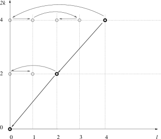
The path of recursion which follows from this procedure is shown in Fig. 1.

V Exploiting the symmetries

As seen above we already have to solve nine ordinary differential equations for the first-order imaginary-time evolution amplitude. For any order $n$ the number $p$ of integrals to solve is

$$p=\sum_{j=1}^{2n+1}(2j-1)=4n^{2}+4n+1\,.$$ (42)

Due to the time reversal behaviour (20), the coefficients $c_{2k|l}^{(n)}(\tau)$ show a symmetry, namely:

$$\frac{c_{2k|l}^{(n)}(\tau)}{\sinh^{l}\omega\tau}=\frac{c_{2k|2k-l}^{(n)}(\tau)}{\sinh^{2k-l}\omega\tau}\,.$$ (43)

Exploiting the symmetry (43), we can cut down the number (42) considerably. At first sight it is reduced to

$$p^{\prime}=\sum_{j=1}^{2n+1}j=2n^{2}+3n+1\,,$$ (44)

so there are only six integrals left for the first order. But we can go even further. Employing these symmetries we can eventually change almost all recursive differential equations into purely algebraic ones leaving only $p^{\prime\prime}=(2n+1)$ integrations. So for the first order we are left with three integrations only, namely with equations (33), (38), and (41). These coefficients $c_{4|4}^{(1)}(\tau)$, $c_{2|2}^{(1)}(\tau)$, and $c_{0|0}^{(1)}(\tau)$ are integrated recursively. The other coefficients can then be obtained algebraically: Once we have $c_{4|4}^{(1)}(\tau)$ we also know $c_{4|0}^{(1)}(\tau)$ because of the symmetry (43). Comparing equation (IV) for $k=2,l=4$ and $k=2,l=0$ we then obtain an algebraic equation for $c_{4|1}^{(1)}(\tau)$. The knowledge of $c_{4|1}^{(1)}(\tau)$ gives us $c_{4|3}^{(1)}(\tau)$ because of the symmetry (43) and by comparing (IV) this time for $k=2,l=3$ on the one hand and $k=2,l=1$ on the other hand we are left with an algebraic equation for $c_{4|2}^{(1)}(\tau)$. Thus we get all the coefficients for $k=2$ only by solving one differential equation, namely the one for $c_{4|4}^{(1)}(\tau)$. For $k=1$ the procedure is similar, $k=0$ only generates one coefficient anyway, namely $c_{0|0}^{(1)}(\tau)$, which still has to be solved by evaluating one integral. The new path of recursion is shown in Fig. 2.
So finally three out of the nine first-order coefficients are obtained by integration, three more are clear for symmetry reasons and three come from an algebraic recursion.
We now generalize the algebraic part of our recursion. Consider again the symmetry property (43). Differentiation on both sides yields

$$\frac{\partial c_{2k|l}^{(n)}(\tau)}{\partial\tau}=\frac{1}{\sinh^{2k-2l}\omega\tau}\frac{\partial c_{2k|2k-l}^{(n)}(\tau)}{\partial\tau}$$

$$-2(k-l)\omega\cosh\omega\tau\frac{c_{2k|2k-l}^{(n)}(\tau)}{\sinh^{2k-2l+1}\omega\tau}\,.$$ (45)

Now we substitute for the two partial derivatives according to equation (IV). Solving for the $(l+1)$-st coefficient and shifting the index $l$ down by one we obtain

$$c_{2k|l}^{(n)}(\tau) = -\frac{(l+1)\hbar}{2M\omega}c_{2k+2|l+1}^{(n)}(\tau)+\frac{c_{2k-4|l-5}^{(n-1)}(\tau)}{\hbar\omega l}\,\sinh^{6}\omega\tau$$ (46)

$$+\,\frac{(2k-l+3)(2k-l+2)\hbar}{2M\omega l}\frac{c_{2k+2|2k-l+3}^{(n)}(\tau)}{\sinh^{2k-2l+2}\omega\tau}+\frac{2k-l+2}{l}\frac{c_{2k|2k-l+2}^{(n)}(\tau)}{\sinh^{2k-2l+2}\omega\tau}$$

$$-\,\frac{1}{\hbar\omega l}\frac{c_{2k-4|2k-l-3}^{(n-1)}(\tau)}{\sinh^{2k-2l-4}\omega\tau}-\frac{(2k-2l+2)\cosh\omega\tau}{l}\frac{c_{2k|2k-l+1}^{(n)}(\tau)}{\sinh^{2k-2l+1}\omega\tau}\,,$$

which is the algebraic recursion relation for any non-diagonal coefficient $c_{2k|l}^{(n)}(\tau)$ with $0<l\leq k$. (The coefficients with $k<l<2k$ are then clear for symmetry reasons.) The diagonal coefficients $c_{2k|2k}^{(n)}(\tau)$ still have to be integrated.

VI Combined differential and algebraic equation

We now combine the differential recursion with the algebraic one. As only the diagonal coefficients have to be evaluated by integrating the differential recursive equation, we can even further simplify the solution (31) to our master equation (IV). We only need it for the diagonal coefficients, for which $l+1=2k+1$ is always greater than $2k$. And according to our index rule (ii), coefficients of the shape $c_{2k|2k+1}^{(n)}$ have to be neglected. We get

$$c_{2k|2k}^{(n)}(\tau)=(2k+2)(2k+1)\frac{\hbar}{2M}\int d\tau\frac{c_{2k+2|2k+2}^{(n)}(\tau)}{\sinh^{2}\omega\tau}$$

$$-\,\frac{1}{\hbar}\int d\tau c_{2k-4|2k-4}^{(n-1)}(\tau)\,\sinh^{4}\omega\tau+d_{2k|2k}^{(n)}\,.$$ (47)

Index rules (i) and (iii) still have to be applied, $k$ runs from 0 to $2n$.
Let us quickly summarize the combined differential and algebraic recursion relation considering the first order as an example. Fig. 2 shows all first-order coefficients for the imaginary time evolution amplitude. Each coefficient is represented by a little circle. Now the coefficients on the diagonal line $2k=l$ have to be obtained by referring to equation (VI) together with rules (i) and (iii). These two rules tell us which of the coefficients either from the the same order $n$ or from the previous order $n-1$ have to be integrated and which ones can be put to zero.
Once we have the diagonal coefficients $c_{2k|2k}^{(n)}(\tau)$ we can calculate the off-diagonal ones with $l\leq k$ with the help of equation (46). The coefficients with $k<l<2k$ are then clear for symmetry reasons.
Using the computer algebra programme Maple V R7 we managed to calculate seven perturbative orders of the imaginary-time evolution amplitude which can be found at internet .

VII Free Energy

In this section we obtain perturbative results for the partition function by integrating the diagonal elements of our perturbative expression for the imaginary-time evolution amplitude from the previous sections:

Figure 1: This diagram depicts the path of recursion for $n=1$. We start in the top right hand side corner, which is to be identified with the coefficient $c_{4|4}^{(1)}$ and follow the arrows until reaching the bottom left hand side corner with the coefficient $c_{0|0}^{(1)}$.

Figure 2: This diagram shows which of the first-order coefficients $c_{2k|l}^{(1)}(\tau)$ have to be integrated (bold) and which ones can be obtained by employing symmetry and algebraic recursions (light).

$$Z=\int_{-\infty}^{+\infty}dx(x\,\hbar\beta|x\,0)\,.$$ (48)

From the partition function we then compute the free energy perturbatively:

$$F=-\frac{1}{\beta}\log Z\,.$$ (49)

We have to expand the logarithm in order to obtain a perturbation expansion for the free energy $F$. For the first order we insert (19) together with (II) into (48) and evaluate the integral and for the second order we use, correspondingly, the data from Ref. internet . By taking the logarithm we get with (49) and with the expansion for the logarithm for the free energy to second order

$$F^{(2)}(\beta)=\frac{1}{\beta}\log 2\sinh\frac{\hbar\beta\omega}{2}$$ (50)

$${}+\frac{3g\hbar^{2}}{4M^{2}\omega^{2}}\coth^{2}\frac{\hbar\beta\omega}{2}-\frac{g^{2}\hbar^{3}}{64M^{4}\omega^{5}}\Bigg{(}\frac{54\hbar\beta\omega}{\sinh^{4}\frac{\hbar\beta\omega}{2}}$$

$${}+\frac{36\hbar\beta\omega\cosh\hbar\beta\omega+60\sinh\hbar\beta\omega+21\sinh 2\hbar\beta\omega}{\sinh^{4}\frac{\hbar\beta\omega}{2}}\Bigg{)}\,.$$

The higher orders are omitted for the sake of keeping the type face clear.
With Maple we came as high as the fifth variational order which is two orders more than what has been obtained in previous work Meyer .

VIII Diagrammatical Check

It is possible to check the perturbative results for the free energy for all temperatures. Namely, we can expand $Z$ in terms of harmonic expectations in a similar way as for the imaginary-time evolution amplitude in (II). To that end we need the generating functional

$$Z[j(\tau)] = \int_{-\infty}^{+\infty}dx(x\,\hbar\beta|x\,0)_{\omega}[j]\,$$ (51)

which we get from (7)-(II). It is of the form

$$Z[j(\tau)]=Z[0]$$ (52)

$$\times\exp\left[\frac{1}{2\hbar^{2}}\int_{0}^{\hbar\beta}d\tau_{1}\int_{0}^{\hbar\beta}d\tau_{2}G^{\rm(p)}(\tau_{1},\tau_{2})j(\tau_{1})j(\tau_{2})\right]\,,$$

where the harmonic partition function reads

$$Z[0]=\frac{1}{2\sinh\frac{\hbar\beta\omega}{2}}$$ (53)

and

$$G^{\rm(p)}(\tau_{1},\tau_{2})=\frac{\hbar}{2M\omega}\frac{\cosh\left(\frac{\hbar\beta\omega}{2}-|\tau_{1}-\tau_{2}|\omega\right)}{\sinh\frac{\hbar\beta\omega}{2}}\,$$ (54)

denotes the periodic Green’s function of the harmonic oscillator. We now obtain the partition function $Z$ of the anharmonic oscillator from the generating functional $Z[j(\tau)]$ by differentiating with respect to the current $j(\tau)$ while setting $j(\tau)=0$ afterwards:

$$Z=\exp\left\{-\frac{1}{\hbar}\int_{0}^{\hbar\beta}d\tau\,g\left[\frac{\hbar\delta}{\delta j(\tau)}\right]^{4}\right\}Z[j(\tau)]\Bigg{|}_{j=0}\,.$$ (55)

Thus we get

$$Z=Z[0]\left\{1-\frac{3g}{\hbar}\int_{0}^{\hbar\beta}d\tau_{1}G^{\rm(p)^{2}}(\tau_{1},\tau_{1})\right.$$ (56)

$${}+\frac{g^{2}}{2\hbar^{2}}\int_{0}^{\hbar\beta}d\tau_{1}\int_{0}^{\hbar\beta}d\tau_{2}\left[9G^{\rm(p)^{2}}(\tau_{1},\tau_{1})G^{\rm(p)^{2}}(\tau_{2},\tau_{2})\right.$$

$$\left.\left.{}+72G^{\rm(p)}(\tau_{1},\tau_{1})G^{\rm(p)^{2}}(\tau_{1},\tau_{2})G^{\rm(p)}(\tau_{2},\tau_{2})\right.\right.$$

$$\left.\left.{}+24G^{\rm(p)^{4}}(\tau_{1},\tau_{2})\right]+...\right\}\,.$$

In terms of Feynman diagrams this reads

$$Z=Z[0]\left[1-\frac{3g}{\hbar}\hskip 2.84526pt\parbox{28.45274pt}{\centerline{\hbox{ \begin{picture}(10.0,10.0)\immediate\ignorespaces\immediate\ignorespaces\immediate\ignorespaces\immediate\ignorespaces\immediate\ignorespaces\put(0.0,0.0){\includegraphics{weissbach.13}}\ignorespaces\immediate\ignorespaces\immediate\ignorespaces\immediate\ignorespaces\immediate\ignorespaces\immediate\ignorespaces\immediate\ignorespaces\immediate\ignorespaces\immediate\ignorespaces\immediate\ignorespaces\immediate\ignorespaces\immediate\ignorespaces\immediate\ignorespaces\immediate\ignorespaces\immediate\ignorespaces\immediate\ignorespaces \immediate\ignorespaces{}\end{picture}}}}\hskip 2.84526pt\right.$$ (57)

$$\left.{}+\frac{g^{2}}{2\hbar^{2}}\left(9\hskip 2.84526pt\parbox{28.45274pt}{\centerline{\hbox{ \begin{picture}(10.0,10.0)\immediate\ignorespaces\immediate\ignorespaces\immediate\ignorespaces\immediate\ignorespaces\immediate\ignorespaces\put(0.0,0.0){\includegraphics{weissbach.14}}\ignorespaces\immediate\ignorespaces\immediate\ignorespaces\immediate\ignorespaces\immediate\ignorespaces\immediate\ignorespaces\immediate\ignorespaces\immediate\ignorespaces\immediate\ignorespaces\immediate\ignorespaces\immediate\ignorespaces\immediate\ignorespaces\immediate\ignorespaces\immediate\ignorespaces\immediate\ignorespaces\immediate\ignorespaces \immediate\ignorespaces{}\end{picture}}}}\hskip 2.84526pt\parbox{28.45274pt}{\centerline{\hbox{ \begin{picture}(10.0,10.0)\immediate\ignorespaces\immediate\ignorespaces\immediate\ignorespaces\immediate\ignorespaces\immediate\ignorespaces\put(0.0,0.0){\includegraphics{weissbach.15}}\ignorespaces\immediate\ignorespaces\immediate\ignorespaces\immediate\ignorespaces\immediate\ignorespaces\immediate\ignorespaces\immediate\ignorespaces\immediate\ignorespaces\immediate\ignorespaces\immediate\ignorespaces\immediate\ignorespaces\immediate\ignorespaces\immediate\ignorespaces\immediate\ignorespaces\immediate\ignorespaces\immediate\ignorespaces \immediate\ignorespaces{}\end{picture}}}}\right.\right.$$

$$\left.\left.+\,72\hskip 2.84526pt\parbox{42.67912pt}{\centerline{\hbox{ \begin{picture}(15.0,10.0)\immediate\ignorespaces\immediate\ignorespaces\immediate\ignorespaces\immediate\ignorespaces\immediate\ignorespaces\put(0.0,0.0){\includegraphics{weissbach.16}}\ignorespaces\immediate\ignorespaces\immediate\ignorespaces\immediate\ignorespaces\immediate\ignorespaces\immediate\ignorespaces\immediate\ignorespaces\immediate\ignorespaces\immediate\ignorespaces\immediate\ignorespaces\immediate\ignorespaces\immediate\ignorespaces\immediate\ignorespaces\immediate\ignorespaces\immediate\ignorespaces\immediate\ignorespaces\immediate\ignorespaces\immediate\ignorespaces\immediate\ignorespaces \immediate\ignorespaces{}\end{picture}}}}\hskip 2.84526pt+24\hskip 2.84526pt\parbox{28.45274pt}{\centerline{\hbox{ \begin{picture}(10.0,10.0)\immediate\ignorespaces\immediate\ignorespaces\immediate\ignorespaces\immediate\ignorespaces\immediate\ignorespaces\put(0.0,0.0){\includegraphics{weissbach.17}}\ignorespaces\immediate\ignorespaces\immediate\ignorespaces\immediate\ignorespaces\immediate\ignorespaces\immediate\ignorespaces\immediate\ignorespaces\immediate\ignorespaces\immediate\ignorespaces\immediate\ignorespaces\immediate\ignorespaces\immediate\ignorespaces\immediate\ignorespaces\immediate\ignorespaces\immediate\ignorespaces\immediate\ignorespaces\immediate\ignorespaces \immediate\ignorespaces{}\end{picture}}}}\hskip 2.84526pt\right)+...\right]$$

$$=\exp\left[\frac{1}{2}\hskip 2.84526pt\parbox{14.22636pt}{\centerline{\hbox{ \begin{picture}(5.0,5.0)\immediate\ignorespaces\immediate\ignorespaces\immediate\ignorespaces\immediate\ignorespaces\immediate\ignorespaces\put(0.0,0.0){\includegraphics{weissbach.18}}\ignorespaces\immediate\ignorespaces\immediate\ignorespaces\immediate\ignorespaces\immediate\ignorespaces\immediate\ignorespaces\immediate\ignorespaces\immediate\ignorespaces\immediate\ignorespaces\immediate\ignorespaces\immediate\ignorespaces\immediate\ignorespaces\immediate\ignorespaces \immediate\ignorespaces{}\end{picture}}}}\hskip 2.84526pt-\frac{3}{\hbar}\hskip 2.84526pt\parbox{28.45274pt}{\centerline{\hbox{ \begin{picture}(10.0,10.0)\immediate\ignorespaces\immediate\ignorespaces\immediate\ignorespaces\immediate\ignorespaces\immediate\ignorespaces\put(0.0,0.0){\includegraphics{weissbach.19}}\ignorespaces\immediate\ignorespaces\immediate\ignorespaces\immediate\ignorespaces\immediate\ignorespaces\immediate\ignorespaces\immediate\ignorespaces\immediate\ignorespaces\immediate\ignorespaces\immediate\ignorespaces\immediate\ignorespaces\immediate\ignorespaces\immediate\ignorespaces\immediate\ignorespaces\immediate\ignorespaces\immediate\ignorespaces \immediate\ignorespaces{}\end{picture}}}}\hskip 2.84526pt\right.$$

$$\left.{}+\frac{g^{2}}{2\hbar^{2}}\left(72\hskip 2.84526pt\parbox{42.67912pt}{\centerline{\hbox{ \begin{picture}(15.0,10.0)\immediate\ignorespaces\immediate\ignorespaces\immediate\ignorespaces\immediate\ignorespaces\immediate\ignorespaces\put(0.0,0.0){\includegraphics{weissbach.20}}\ignorespaces\immediate\ignorespaces\immediate\ignorespaces\immediate\ignorespaces\immediate\ignorespaces\immediate\ignorespaces\immediate\ignorespaces\immediate\ignorespaces\immediate\ignorespaces\immediate\ignorespaces\immediate\ignorespaces\immediate\ignorespaces\immediate\ignorespaces\immediate\ignorespaces\immediate\ignorespaces\immediate\ignorespaces\immediate\ignorespaces\immediate\ignorespaces\immediate\ignorespaces \immediate\ignorespaces{}\end{picture}}}}\hskip 2.84526pt+24\hskip 2.84526pt\parbox{28.45274pt}{\centerline{\hbox{ \begin{picture}(10.0,10.0)\immediate\ignorespaces\immediate\ignorespaces\immediate\ignorespaces\immediate\ignorespaces\immediate\ignorespaces\put(0.0,0.0){\includegraphics{weissbach.21}}\ignorespaces\immediate\ignorespaces\immediate\ignorespaces\immediate\ignorespaces\immediate\ignorespaces\immediate\ignorespaces\immediate\ignorespaces\immediate\ignorespaces\immediate\ignorespaces\immediate\ignorespaces\immediate\ignorespaces\immediate\ignorespaces\immediate\ignorespaces\immediate\ignorespaces\immediate\ignorespaces\immediate\ignorespaces\immediate\ignorespaces \immediate\ignorespaces{}\end{picture}}}}\hskip 2.84526pt\right)+...\right]\,,$$ (58)

where we have introduced the symbol

$$\frac{1}{2}\hskip 2.84526pt\parbox{14.22636pt}{\centerline{\hbox{ \begin{picture}(5.0,5.0)\immediate\ignorespaces\immediate\ignorespaces\immediate\ignorespaces\immediate\ignorespaces\immediate\ignorespaces\put(0.0,0.0){\includegraphics{weissbach.22}}\ignorespaces\immediate\ignorespaces\immediate\ignorespaces\immediate\ignorespaces\immediate\ignorespaces\immediate\ignorespaces\immediate\ignorespaces\immediate\ignorespaces\immediate\ignorespaces\immediate\ignorespaces\immediate\ignorespaces\immediate\ignorespaces\immediate\ignorespaces \immediate\ignorespaces{}\end{picture}}}}\hskip 2.84526pt\equiv\log Z[0]\,.$$ (59)

Once we rewrite the partition function $Z$ in the form of the cumulant expansion as on the right hand side of equation (57), the disconnected Feynman diagrams disappear Kleinert . Now we can easily take the logarithm. Following (49) we obtain for the free energy

$$F=-\frac{1}{\beta}\left[\frac{1}{2}\hskip 2.84526pt\parbox{14.22636pt}{\centerline{\hbox{ \begin{picture}(5.0,5.0)\immediate\ignorespaces\immediate\ignorespaces\immediate\ignorespaces\immediate\ignorespaces\immediate\ignorespaces\put(0.0,0.0){\includegraphics{weissbach.23}}\ignorespaces\immediate\ignorespaces\immediate\ignorespaces\immediate\ignorespaces\immediate\ignorespaces\immediate\ignorespaces\immediate\ignorespaces\immediate\ignorespaces\immediate\ignorespaces\immediate\ignorespaces\immediate\ignorespaces\immediate\ignorespaces\immediate\ignorespaces \immediate\ignorespaces{}\end{picture}}}}\hskip 2.84526pt-\frac{3g}{\hbar}\hskip 2.84526pt\parbox{28.45274pt}{\centerline{\hbox{ \begin{picture}(10.0,10.0)\immediate\ignorespaces\immediate\ignorespaces\immediate\ignorespaces\immediate\ignorespaces\immediate\ignorespaces\put(0.0,0.0){\includegraphics{weissbach.24}}\ignorespaces\immediate\ignorespaces\immediate\ignorespaces\immediate\ignorespaces\immediate\ignorespaces\immediate\ignorespaces\immediate\ignorespaces\immediate\ignorespaces\immediate\ignorespaces\immediate\ignorespaces\immediate\ignorespaces\immediate\ignorespaces\immediate\ignorespaces\immediate\ignorespaces\immediate\ignorespaces\immediate\ignorespaces \immediate\ignorespaces{}\end{picture}}}}\hskip 2.84526pt\right.$$ (60)

$$\left.{}+\frac{g^{2}}{2\hbar^{2}}\left(72\hskip 2.84526pt\parbox{42.67912pt}{\centerline{\hbox{ \begin{picture}(15.0,10.0)\immediate\ignorespaces\immediate\ignorespaces\immediate\ignorespaces\immediate\ignorespaces\immediate\ignorespaces\put(0.0,0.0){\includegraphics{weissbach.25}}\ignorespaces\immediate\ignorespaces\immediate\ignorespaces\immediate\ignorespaces\immediate\ignorespaces\immediate\ignorespaces\immediate\ignorespaces\immediate\ignorespaces\immediate\ignorespaces\immediate\ignorespaces\immediate\ignorespaces\immediate\ignorespaces\immediate\ignorespaces\immediate\ignorespaces\immediate\ignorespaces\immediate\ignorespaces\immediate\ignorespaces\immediate\ignorespaces\immediate\ignorespaces \immediate\ignorespaces{}\end{picture}}}}\hskip 2.84526pt+24\hskip 2.84526pt\parbox{28.45274pt}{\centerline{\hbox{ \begin{picture}(10.0,10.0)\immediate\ignorespaces\immediate\ignorespaces\immediate\ignorespaces\immediate\ignorespaces\immediate\ignorespaces\put(0.0,0.0){\includegraphics{weissbach.26}}\ignorespaces\immediate\ignorespaces\immediate\ignorespaces\immediate\ignorespaces\immediate\ignorespaces\immediate\ignorespaces\immediate\ignorespaces\immediate\ignorespaces\immediate\ignorespaces\immediate\ignorespaces\immediate\ignorespaces\immediate\ignorespaces\immediate\ignorespaces\immediate\ignorespaces\immediate\ignorespaces\immediate\ignorespaces\immediate\ignorespaces \immediate\ignorespaces{}\end{picture}}}}\hskip 2.84526pt\right)+...\right]\,.$$

The above Feynman diagrams are of course constructed with the help of the same rules as for the imaginary-time evolution amplitude (12), (13), and (14), but instead of the Dirichlet’s Green’s function (II) we have to use the periodic Green’s function (54). We now want to evaluate the four diagrams in (60) so that we get a second-order expression for the free energy for finite temperatures. According to (53) and (59) we get for the zeroth-order contribution

$$\frac{1}{2}\hskip 2.84526pt\parbox{14.22636pt}{\centerline{\hbox{ \begin{picture}(5.0,5.0)\immediate\ignorespaces\immediate\ignorespaces\immediate\ignorespaces\immediate\ignorespaces\immediate\ignorespaces\put(0.0,0.0){\includegraphics{weissbach.27}}\ignorespaces\immediate\ignorespaces\immediate\ignorespaces\immediate\ignorespaces\immediate\ignorespaces\immediate\ignorespaces\immediate\ignorespaces\immediate\ignorespaces\immediate\ignorespaces\immediate\ignorespaces\immediate\ignorespaces\immediate\ignorespaces\immediate\ignorespaces \immediate\ignorespaces{}\end{picture}}}}\hskip 2.84526pt=\log\left[\frac{1}{2\sinh\frac{\hbar\beta\omega}{2}}\right]\,,$$ (61)

whereas the first-order diagram becomes

$$\parbox{28.45274pt}{\centerline{\hbox{ \begin{picture}(10.0,10.0)\immediate\ignorespaces\immediate\ignorespaces\immediate\ignorespaces\immediate\ignorespaces\immediate\ignorespaces\put(0.0,0.0){\includegraphics{weissbach.28}}\ignorespaces\immediate\ignorespaces\immediate\ignorespaces\immediate\ignorespaces\immediate\ignorespaces\immediate\ignorespaces\immediate\ignorespaces\immediate\ignorespaces\immediate\ignorespaces\immediate\ignorespaces\immediate\ignorespaces\immediate\ignorespaces\immediate\ignorespaces\immediate\ignorespaces\immediate\ignorespaces\immediate\ignorespaces \immediate\ignorespaces{}\end{picture}}}}\hskip 2.84526pt=\frac{\hbar^{3}\beta}{4M^{2}\omega^{2}}\coth^{2}\frac{\hbar\beta\omega}{2}\,.$$ (62)

The integration in (62) is trivial, because $G^{(\rm p)}(\tau,\tau)$ does not depend on $\tau$ any more according to (54). For the second order the integrations become more sophisticated:

$$\parbox{42.67912pt}{\centerline{\hbox{ \begin{picture}(15.0,10.0)\immediate\ignorespaces\immediate\ignorespaces\immediate\ignorespaces\immediate\ignorespaces\immediate\ignorespaces\put(0.0,0.0){\includegraphics{weissbach.29}}\ignorespaces\immediate\ignorespaces\immediate\ignorespaces\immediate\ignorespaces\immediate\ignorespaces\immediate\ignorespaces\immediate\ignorespaces\immediate\ignorespaces\immediate\ignorespaces\immediate\ignorespaces\immediate\ignorespaces\immediate\ignorespaces\immediate\ignorespaces\immediate\ignorespaces\immediate\ignorespaces\immediate\ignorespaces\immediate\ignorespaces\immediate\ignorespaces\immediate\ignorespaces \immediate\ignorespaces{}\end{picture}}}}\hskip 2.84526pt=\frac{\hbar^{5}\beta\coth^{2}\frac{\hbar\beta\omega}{2}}{32M^{4}\omega^{5}\sinh^{2}\frac{\hbar\beta\omega}{2}}$$

$$\times(\hbar\beta\omega+\sinh\hbar\beta\omega)\,.$$

The other contribution to the second order yields

$$\parbox{28.45274pt}{\centerline{\hbox{ \begin{picture}(10.0,10.0)\immediate\ignorespaces\immediate\ignorespaces\immediate\ignorespaces\immediate\ignorespaces\immediate\ignorespaces\put(0.0,0.0){\includegraphics{weissbach.30}}\ignorespaces\immediate\ignorespaces\immediate\ignorespaces\immediate\ignorespaces\immediate\ignorespaces\immediate\ignorespaces\immediate\ignorespaces\immediate\ignorespaces\immediate\ignorespaces\immediate\ignorespaces\immediate\ignorespaces\immediate\ignorespaces\immediate\ignorespaces\immediate\ignorespaces\immediate\ignorespaces\immediate\ignorespaces\immediate\ignorespaces \immediate\ignorespaces{}\end{picture}}}}\hskip 2.84526pt=\frac{\hbar^{5}\beta}{256M^{4}\omega^{5}\sinh^{4}\frac{\hbar\beta\omega}{2}}$$ (65)

$$\times(\sinh 2\hbar\beta\omega+8\sinh\hbar\beta\omega+6\hbar\beta\omega)\,.$$

So all in all we get for the free energy (60) up to second order in the coupling constant $g$ the result (50). It shows the correct low-temperature behaviour

$$\lim_{\beta\rightarrow\infty}F^{(2)}(\beta)=\frac{\hbar\omega}{2}+\frac{3g\hbar^{2}}{4M^{2}\omega^{2}}-\frac{21g^{2}\hbar^{3}}{8M^{4}\omega^{5}}\,,$$ (66)

which is the ground state energy and can be found for instance in Bender/Wu ; Kleinert .

IX Variational Perturbation Theory

Variational perturbation theory is a method that enables us to resum divergent Borel-type perturbation series in such a way that they converge even for infinitely large values of the perturbative coupling Kleinert ; Frohlinde . To this end we add and subtract a trial harmonic oscillator with trial frequency $\Omega$ to our anharmonic oscillator (2):

$$V(x)=\frac{M}{2}\Omega^{2}x^{2}+g\frac{M}{2}\frac{\omega^{2}-\Omega^{2}}{g}x^{2}+gx^{4}\,.$$ (67)

Now we treat the second term as if it was of the order of the coupling constant $g$. The result is obtained most simply by substituting for the frequency $\omega$ in the original anharmonic oscillator potential (2) according to Kleinert’s square-root trick Kleinert

$$\omega\rightarrow\Omega\sqrt{1+gr}\,,$$ (68)

where

$$r\equiv\frac{\omega^{2}-\Omega^{2}}{g\Omega^{2}}\,.$$ (69)

These substitutions are not the most general ones. The square root is just a special case for the anharmonic oscillator.
We now apply the trick (68) to our first-order series representation for the free energy $F$ found in (50). Substituting for the frequency $\omega$ according to (68), expanding for fixed $r$ up to the first order in $g$ and re-substituting for $r$ according to (69) we get

$$F^{(1)}(\beta,\Omega)=-\frac{1}{\beta}\log\frac{1}{2\sinh\frac{\hbar\beta\Omega}{2}}+\frac{3g\hbar^{2}}{4M^{2}\Omega^{2}}\coth^{2}\frac{\hbar\beta\Omega}{2}$$

$${}+\frac{\hbar\Omega}{4}\left(\frac{\omega^{2}}{\Omega^{2}}-1\right)\coth\frac{\hbar\beta\Omega}{2}\,.$$ (70)

So the free energy (IX) now depends on the trial frequency $\Omega$ which is of no physical relevance. In order to get rid of it, we have to minimize its effect by employing the principle of least sensitivity Stevenson . This principle suggests to search for local extrema of $F(\beta,\Omega)$ with respect to $\Omega$:

$$\frac{\partial F^{(1)}(\beta,\Omega)}{\partial\Omega}=0\,.$$ (71)

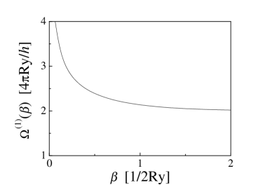
For the first order $F^{(1)}(\beta,\Omega)$ it turns out that there are several extrema for each $\beta$. As we seek a curve $\Omega^{(1)}(\beta)$ that is as smooth as possible the choice is easy — we take the lowest branch for the others are not bounded (see Fig. 3). Moreover the other branches lead to diverging results.
To second order, we proceed in a similar way and we find that there are no extrema at all for $F^{(2)}(\beta,\Omega)$. In accordance with the principle of least sensitivity we look for inflection points instead, i.e. we look for solutions to the equation

$$\frac{\partial^{2}F^{(2)}(\beta,\Omega)}{\partial\Omega^{2}}=0\,.$$ (72)

In general we try to solve the equation

$$\frac{\partial^{n}F^{(N)}(\beta,\Omega)}{\partial\Omega^{n}}=0\,$$ (73)

for the smallest possible $n$. Plugging $\Omega^{(N)}(\beta)$ into $F^{(N)}(\beta,\Omega)$, we finally get back a re-summed expression for the physical quantity $F(\beta)$. The results for the first three orders are given in Fig. 4.

Figure 3: Branch of the variational parameter $\Omega^{(1)}(\beta)$ which we chose. The coupling strength is $g=1$. Other branches not shown in this figure lead to highly diverging results. Throughout this paper all results are presented in natural units $\hbar=k_{\rm B}\equiv 1$ and, additionally, we have set $M=\omega\equiv 1$.

Figure 4: Free energy of the anharmonic oscillator up to third order for intermediate coupling $g=1$. The solid line represents the numerical result $F^{(9)}_{\rm num}(\beta)$, obtained by approximating the partition function (75) with the help of the first ten energy eigenvalues. The other lines are variational perturbative results: The dashed line shows the first order, the dotted line shows the second order, and the dot-dashed line represents the third order. Note that the second and third order are hardly distinguishable from the numerical results. Higher orders for a special value of the inverse temperature $\beta$ can be found in Fig. 5.

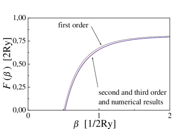
In order to check our results we have to compare them to the numerically evaluated free energy $F^{(N)}_{\rm num}(\beta)$ which is discussed in Sec. XI.

X Higher Orders

We now evaluate the convergence behaviour for the variational perturbative results for the free energy $F^{(N)}(\beta)$ up to the fifth order. However, in order to reduce the computational cost we restrict ourselves to a certain value of the inverse temperature $\beta$. Results are shown in Fig. 5. For odd variational perturbation orders we optimized the free energy according to (71), i.e. we determined $\Omega$ by setting the first derivative of $F^{(N)}(\beta)$ with respect to $\Omega$ to zero. For even orders we had to go for inflection points, instead, so we had to solve equation (72).
It turns out that odd and even orders oscillate about an exponential best fit curve. For $\beta=1$ the numerical result, $F_{\rm num}^{(9)}(1.0)=0.6571$, turns out to lie within the interval obtained by fitting the five perturbative orders of the free energy with origin, as shown in Fig. 5. This interval is $[0.657,0.659]$, and

Figure 5: The free energy of the anharmonic oscillator for intermediate coupling $g=1$ for $\beta=1$ up to fifth variational perturbative order. The values converge exponentially towards the numerical value $F^{(9)}_{{\rm num}}(1)$=0.6571, which is shown as a straight line. The dimension of the free energy in natural units is $2Ry$.

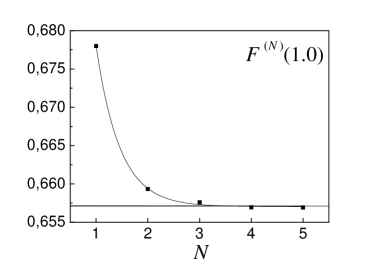
clearly, the variational perturbative results converge exponentially.

XI Checking our Results

The spectral representation of the partition function reads

$$Z=\sum_{n=0}^{\infty}e^{-\beta E_{n}}\,,$$ (74)

where the $E_{n}$ are the energy eigenvalues. Let us define the numerical approximants

$$Z^{(N)}_{\rm num}=\sum_{n=0}^{N}e^{-\beta E_{n}}$$ (75)

and

$$F^{(N)}_{\rm num}=-\frac{1}{\beta}\log Z^{(N)}\,,$$ (76)

respectively. One possibility to obtain numerical results for the eigenvalues $E_{n}$ is provided for by the so called “shooting method”. We integrate the Schrödinger equation numerically for the potential (2) and for a particular value of the coupling strength $g$. If the energy $E$ which we plug into the program does not coincide with one of the energy eigenvalues $E_{n}$, the solution to the Schrödinger equation explodes already for relatively small values of the coordinate $x$. If the energy eigenvalue is close to the exact answer, we have $|\Psi(x)|<\infty$ also for larger values of $x$. This method yields the unnormalized eigenfunctions (the wave functions which still have to be normalized) and the energy eigenvalues to very high accuracy (see Tab. 1). Renormalization is necessary, for the computer algebra programme needs an initial value $\Psi(0)$ which we set to one.

$n$ $E_{n}$ $n$ $E_{n}$ 0 0.8037701932 5 14.203064494 1 2.7378891484 6 17.633934116 2 5.1792814619 7 21.236268598 3 7.9423804544 8 24.994705012 4 10.963538555 9 28.896941521

Table 1: The first ten energy eigenvalues $E_{n}$ of the anharmonic oscillator for intermediate coupling $g=1$. They were obtained by numerically integrating the Schrödinger equation with the initial condition that $\Psi(0)=1$, $\Psi^{\prime}(0)=0$ for even $n$, and $\Psi(0)=0$ and $\Psi^{\prime}(0)=1$ for odd $n$, and of course $|\Psi(x)|<\infty$ for large $x$. The energy eigenvalues are given in units of $2Ry$.

Plugging the first ten numeric energy eigenvalues

Figure 6: The numerial free energy $F_{\rm num}^{(9)}(\beta)$, the first-order variational perturbative results for the free energy $F^{(1)}(\beta)$, and the classical free energy $F_{\rm cl}(\beta)=-(\log Z_{\rm cl})/\beta$, from top to bottom. For small values of the inverse temperature $\beta$ the classical calculations coincide with the other results. Lower temperatures, corresponding to higher values of $\beta$, reveal differences between the classical approach (XI) and quantum statistics.

into equation (75) and evaluating (76) up to $N=9$, we obtain a function $F^{(N)}_{{\rm num}}(\beta)$. It converges rapidly for low temperatures, corresponding to high values of $\beta$. For high temperatures more terms should be taken into account.
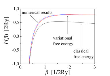
Alternatively one can also use classical results as a high-temperature cross check: High temperatures correspond to classical statistical distributions such that we can evaluate the classical partition function according to

$$Z_{\rm cl}=\int_{-\infty}^{+\infty}\frac{dx}{\lambda_{\rm th}}\exp\left[-\beta V(x)\right]\,,$$ (77)

with the potential (2) and $\lambda_{\rm th}=\sqrt{2\pi\hbar^{2}/Mk_{\rm B}T}$. This integral reduces to

$$Z_{\rm cl}=\frac{1}{2\lambda_{\rm th}}\sqrt{\frac{M\omega^{2}}{2g}}$$

$$\times\exp\left(\frac{\beta M^{2}\omega^{4}}{32g}\right)K_{1/4}\left(\frac{\beta M^{2}\omega^{4}}{32g}\right)\,,$$ (78)

where $K_{1/4}(z)$ is a modified Bessel function. The classical partition function (XI) can be evaluated for high temperatures which corresponds to small values of $\beta$. Consequently, when we test our variational perturbative results, we compare them to the classical free energy for low values of $\beta$, namely $\beta<1/4$. And for high values of $\beta$ we use the numerical approximation, $F^{(9)}_{\rm num}(\beta)$, for comparison (see Fig. 6).
In natural units $\hbar=k_{\rm B}=1$ a value of $\beta=1/4$ corresponds to a physical temperature of $T=1.26\times 10^{6}K$.

XII Conclusion and Outlook

The recursive technique that has been developed throughout Sections IV–VI definitely out classes all diagrammatical perturbative calculations. Using the conventional evaluation of Feynman diagrams, the partition function and the free energy have been evaluated up to third order Meyer , here we obtained the fifth-order result.
For the free energy the convergence of variational perturbation theory was found to be exponential. The fact that the principle of least sensitivity Stevenson produces extrema for the odd variational orders and inflection points for even orders is reflected in the respective convergence behaviours: Odd and even orders can best be fitted separately by exponentials as emphasized in Ref. Frohlinde . Thus we obtained intervals of convergence for certain values of the free energy which always turned out to contain the exact numerical result when taking into account the statistical errors associated with the boundaries of the intervals. For the free energy, the numerical results were obtained using its spectral representation reverting on the first ten energy eigenvalues obtained with the “shooting method”, sketched in Sec. XI.
Finally, we note that our high-order perturbative results for the anharmonic imaginary-time evolution amplitude are useful for calculating other thermodynamic quantities as the correlation function or the ground state wave function weissbach ; ref2 ; Kunihiro . Furthermore, it remains to compare these perturbative results with the semiclassical approximation ref1 .