Quasifree Eta Photoproduction from Nuclei

Abstract

Quasifree $\eta$ photoproduction from nuclei is studied in the Distorted Wave Impulse Approximation (DWIA). The elementary eta production operator contains Born terms, vector meson and nucleon resonance contributions and provides an excellent description of the recent low energy Mainz measurements on the nucleon. The resonance sector includes the $S_{11}(1535)$, $P_{11}(1440)$ and $D_{13}(1520)$ states whose couplings are fixed by independent electromagnetic and hadronic data. Different models for the $\eta N$ t-matrix are used to construct a simple $\eta A$ optical potential based on a $t\rho$-approximation. We find that the exclusive $A(\gamma,\eta N)B$ process can be used to study medium modifications of the $N^{*}$ resonances, particularly if the photon asymmetry can be measured. The inclusive $A(\gamma,\eta)X$ reaction is compared to new data obtained on ${}^{12}C$, ${}^{40}Ca$, and is found to provide a clear distinction between different models for the $\eta N$ t-matrix.

I Introduction

Photoproduction of the isoscalar eta meson with mass of approximately 550 MeV offers the possibility of investigating the $\eta N$- and $\eta A$-interaction, as well as the basic production amplitude. Recently it has been suggested by Wilkin[1] that the very large production cross sections found in the $pd\rightarrow\eta^{3}He$ reaction near threshold could be due to an $\eta N$ scattering length that is much larger than the value extracted from a coupled-channels analysis of the $\pi^{-}p\rightarrow\eta n$ and $\pi N\rightarrow\pi N$ data[2]. Based on the K-matrix formalism, Wilkin was able to reproduce the strong threshold energy dependence of $pd\rightarrow\eta^{3}He$ by assuming an $\eta N$ scattering length with a real part more than twice as large as in previous analyses. Should this conclusion turn out to be true, it would have dramatic implications for the $\eta$-nucleus interaction. Most importantly, a larger value for the scattering length might indicate a larger probability for the presence of a “bound” $\eta$-state for lighter nuclei such as ³He than had been expected. In fact, this seems to be required to explain the cusp-like structure seen for near-threshold production in the $pd\rightarrow{{}^{3}He}X$ reaction for a missing mass close to the $\eta$-mass. This effect may also remove the discrepancy between experiment and theory for the reaction ${}^{3}He(\pi^{-},\eta)^{3}H$[3].

Over the last several years there has been renewed interest in the production of $\eta$–mesons with protons, pions and electrons and their interaction with nucleons and nuclei. One of the first $\eta$–nuclear experiments, performed at SATURNE in 1988[4], reported surprisingly large eta production rates near threshold in the reaction $p(\vec{d},^{3}He)\eta$. These large cross sections permitted not only a more precise determination of the $\eta$–mass[5] but were also used to perform rare decay measurements of the eta[6]. Additional experiments involving pion induced eta production were performed at Los Alamos[7]. Again, the experimental cross sections at threshold region of the reaction ³He($\pi^{-},\eta$)³H are above the theoretical calculations[3, 7].

The advent of high duty-cycle electron accelerators opens for the first time the opportunity to study the reactions $N(\gamma,\eta)N$ and $N(e,e^{\prime}\eta)N$ in greater detail. Our present knowledge of the $(\gamma,\eta)$ process is based solely on some old measurements around 20 years ago[8], along with very few more recent data from Bates[9] and Tokyo[10]. Over the last two years eta photoproduction from the nucleon has been measured at Mainz and at Bonn with an accuracy of more than an order of magnitude better than in older experiments. At Mainz, the TAPS collaboration has obtained high-quality data for angular distributions and total cross sections for photon energies between threshold and 790 MeV both on the nucleon [11] and on nuclear targets ${}^{12}C$, ${}^{40}Ca$ [12]. That may be considered to be a qualitative breakthrough in the experimental field. Similarly, data at the higher energies up to 1150 MeV will be provided soon by the Phoenics collaboration at ELSA [13].

In this work we present a study of the quasifree eta photoproduction on nuclei $A(\gamma,\eta N)B$ (where $B$ is some discrete nuclear state) in the Distorted Wave Impulse Approximation (DWIA). The model allows for the study of the production process and the final-state interactions without being obscured by the details of nuclear transition densities, unlike the reaction of the type $A(\gamma,\eta)B$ where nuclear transition densities play an important role. This is mainly due to the quasifree nature of the reaction: the momentum transfer to the residual nucleus can be made small. The key ingredients of the model are a) the single particle wave functions and spectroscopic factors, b) the elementary eta photoproduction amplitudes, and c) the final state interactions. Information on each ingredient can be taken directly from independent studies. Previous studies of such quasifree reactions on the pion have proven to be successful [14, 15, 16]. Other studies on eta photoproduction from nuclei can be found, for example, in Refs. [17, 18, 19, 20, 21, 22, 23].

In Sec. II we briefly describe the $(\gamma,\eta)$ operator and show comparisons with new data from Mainz. The DWIA formalism for quasifree eta photoproduction on nuclei is derived in Sec. III. In Sec. IV we present predictions for differential cross sections of the exclusive reaction $A(\gamma,\eta N)B$. In Sec. V we compare our calculations with new data from Mainz on the inclusive reaction $A(\gamma,\eta)X$. In Sec. VI we summarize our findings and present a brief outlook. The transformation of CGLN amplitudes from the c.m. frame to an arbitrary reference frame is given in the Appendix. The transformation is needed to implement the elementary amplitudes in nuclear calculations.

II Eta photoproduction on the nucleon

Nucleon resonance excitation is the dominant reaction process in $(\gamma,\eta)$. In contrast to pions which will excite $\Delta(T=3/2)$ as well as $N^{*}(T=1/2)$ resonances, the $\eta$ meson will only appear in the decay of $N^{*}$ resonances with $T=1/2$. In the low-energy region this is dominantly the $S_{11}(1535)$ state that decays 45-55% into $\eta N$, the only nucleon resonance with such a strong branching ratio in the $\eta$ channel. This result is even more surprising as a nearby resonance of similar structure, the $S_{11}(1650)$ has a branching ratio of only 1.5%. The other resonances that play roles in the low energy region are the $P_{11}(1440)$ and $D_{13}(1520)$.

Most attempts to describe eta photoproduction on the nucleon[24, 25] have involved Breit–Wigner functions for the resonances and either phenomenology or an effective Lagrangian approach to model the background. These models which contain a large number of free parameters were then adjusted to reproduce the few available data. In a very different approach, Ref. [26] derived a dynamical model which employs $\pi N\rightarrow\pi N,\pi N\rightarrow\pi\pi N$ and $\pi^{-}p\rightarrow\eta n$ to fix the hadronic vertex as well as the propagators and the $\gamma N\rightarrow\pi N$ to construct the electromagnetic vertex. This calculation represents a prediction rather than a fit to the $\gamma N\rightarrow\eta N$ reaction. The model was later extended to include the background from $s,u$–channel nucleon Born terms and $\rho,\omega$ exchange in the $t$–channel [27]. Due to the fact that $\eta$ is an isoscalar meson, two coupling schemes are possible at the $\eta NN$ vertex: pseudovector(PV) and pseudoscalar(PS). The latter one is not ruled out by LET as in the case of $(\gamma,\pi)$. Since the resonance sector is fixed in this approach and also the vector meson couplings can be obtained from independent sources, one can use this model to determine the nature of $\eta NN$ coupling: both the coupling scheme and the coupling constant.

In contrast to the $\pi N$-interaction, little is known about the $\eta N$-interaction and, consequently, about the $\eta NN$ vertex. The uncertainty regarding the structure of the $\eta NN$ vertex extends to the magnitude of the coupling constant. This coupling constant $g_{\eta NN}^{2}/4\pi$ varies between $0$ and $7$ with the large couplings arising from fits of one boson exchange potentials [28]. ¿From SU(3) flavor symmetry, all coupling constants between the meson octet and the baryon octet are determined by one free parameter $\alpha$, giving

$$\frac{g_{\eta NN}^{2}}{4\pi}=\frac{1}{3}(3-4\alpha)^{2}\;\frac{g_{\pi NN}^{2}}{4\pi}\;,$$ (1)

resulting in values for the coupling constant between $0.8$ and $1.9$ for commonly used values of $\alpha$ between $0.6-0.65$, depending on the F and D strengths chosen as the two types of SU(3) octet meson-baryon couplings. Other determinations of the $\eta NN$ coupling employ reactions involving the eta, such as $\pi^{-}p\rightarrow\eta n$, and range from 0.6 - 1.7[29]. Smaller values are supported by $NN$ forward dispersion relations[30] with $g_{\eta NN}^{2}/{4\pi}+g_{\eta^{\prime}NN}^{2}/{4\pi}\leq 1.0$. There is some rather indirect evidence that also favors a small value for $g_{\eta NN}$. In Ref.[31], Piekarewicz calculated the $\pi$–$\eta$ mixing amplitude in the hadronic model where the mixing was generated by $\bar{N}N$ loops and thus driven by the proton–neutron mass difference. To be in agreement with results from chiral perturbation theory the $\eta NN$ coupling had to be constrained to the range 0.32 – 0.53. In a very different approach, Hatsuda[32] evaluated the proton matrix element of the flavor singlet axial current in the large $N_{C}$ chiral dynamics with an effective Lagrangian that included the $U_{A}$(1) anomaly. In this framework, the EMC data on the polarized proton structure function (which have been used to determine the ”strangeness content” of the proton) can be related to the $\eta^{\prime}NN$ and the $\eta NN$ coupling constants. Again, his analysis prefers small values for both coupling constants. Nevertheless, from the above discussion it seems clear that the $\eta NN$ coupling constant is much smaller than the corresponding $\pi NN$ value of around 14.

In Fig. 1, we show the sensitivity of the total cross section close to threshold when varying the coupling constant from 0 to 3 for the PS and from 0 to 10 for the PV form. There is a large variation of more than a factor of 2 at 750 MeV for the PS case while changing the value with PV structure modifies the cross section only by a relatively small amount.

Here the very precise results of the new Mainz experiment can clearly distinguish between the different models preferring a pseudoscalar coupling scheme with a best-fit coupling constant of $g_{\eta NN}^{2}/4\pi$=0.4. This is further supported by comparing with the differential cross section as shown in Fig. 2. There is a clear distinction in the forward-backward asymmetry of the angular distribution between the PS- and PV-model, and PS coupling with $g_{\eta NN}^{2}/4\pi$=0.4 is strongly supported. The variation in the angular distributions is due to the $p$-wave multipoles. In particular, the $M_{1-}$ multipole changes sign between PS and PV coupling.

Fig. 3 shows the complete view of the differential cross section and the photon asymmetry of $\eta$ photoproduction on the proton from threshold up to 800 MeV for PS coupling with $g_{\eta NN}^{2}/4\pi$=0.4. The resonance dominance near threshold is clearly seen in the cross section. The angular distribution is relatively flat in the cross section but peaked in the photon asymmetry.

III DWIA model for $\eta$ photoproduction from nuclei

A Kinematics

In this section we define our coordinate system and discuss some kinematic aspects of the exclusive reaction $(\gamma,\eta N)$ and the inclusive reaction $(\gamma,\eta)$ on nuclei. In the laboratory frame, the four-momenta of the incoming photon is $k^{\mu}=(E_{\gamma},{\bf k})$ while the outgoing eta and nucleon have four-momenta of $q^{\mu}=(E_{\eta},{\bf q})$ and $p^{\mu}=(E_{N},{\bf p})$ respectively. The target nucleus is at rest with mass $M_{i}$ and the recoiling residual nucleus of mass $M_{f}$ has momentum

$${\bf Q}={\bf k}-{\bf q}-{\bf p}$$ (2)

and kinetic energy $T_{Q}=\frac{Q^{2}}{2M_{f}}$. The momentum transfer ${\bf Q}$ is sometimes also called the missing momentum. Overall energy conservation requires

$$E_{\gamma}+M_{i}=E_{\eta}+E_{N}+M_{f}+T_{Q}.$$ (3)

As shown in Fig. 4, the z-axis is defined by the photon direction ${\bf k}$, and we choose the azimuthal angle of the eta, $\phi_{\eta}=0$, by defining ${\bf\hat{y}}={\bf\hat{k}}\times{\bf\hat{q}}$ and ${\bf\hat{x}}={\bf\hat{y}}\times{\bf\hat{z}}$.

We assume that the reaction takes place on a single bound nucleon with four -momentum $p{{}^{\mu}}{{}_{i}}=(E_{i},{\bf p}_{i})$ and that energy and momentum are conserved at this vertex (i.e., the impulse approximation). Thus ${\bf p}_{i}=-{\bf Q}$ and $E_{i}=E_{\eta}+E_{N}-E_{\gamma}$. If ${\bf Q}$ does not vanish, the struck nucleon is off its mass shell. For exclusive reactions this is the only reasonable off-shell choice since the photon, the eta, the outgoing nucleon, and the recoiling nucleus are all external lines and must be on their respective mass shells. For the inclusive reaction we make the same choice.

The magnitude of the momentum transfer to the recoiling nucleus has a wide range, including zero, depending on the directions of the outgoing eta and nucleon with respect to the incident photon beam. However, since the reaction amplitude is proportional to the Fourier transform of the bound state single particle wavefunction, it becomes quite small for momentum transfers greater than about 300 MeV/c. Thus for all but the lightest nuclei we can safely neglect the nuclear recoil velocity and generate optical potentials for the outgoing particles in the laboratory frame. As noted in [14], reactions of the form $(\gamma,\eta N)$ on nuclei offer great kinematic flexibility and by appropriate choices one can investigate the production operator, the bound state wavefunction, or the final state interaction of the outgoing meson and nucleon.

B The DWIA cross sections

In this section we give the DWIA formalism for calculating the quasifree eta photoproduction from nuclei. Following standard procedure, the differential cross section is given by

$$d\sigma=\frac{1}{2E_{\gamma}}\bar{\sum}|{\cal M}_{fi}|^{2}(2\pi)^{4}\delta^{4}(P_{f}+p+q-P_{i}-k)\frac{d{\bf q}}{2E_{\eta}(2\pi)^{3}}\frac{m_{p}d{\bf p}}{E_{p}(2\pi)^{3}}\frac{M_{f}d{\bf Q}}{E_{f}(2\pi)^{3}}$$ (4)

where $\bar{\sum}$ means sums over final spins and average over initial spins. The $\delta$-function ensures overall energy-momentum conservation. In impulse approximation, the many-body matrix element can be written as a sum over single particle states $\alpha=\{nljm\}$

$${\cal M}_{fi}=\sum_{\alpha}\langle J_{f},m_{f}|a_{\alpha}|J_{i},m_{i}\rangle\langle\eta;N|t_{\gamma\eta}|\alpha;\gamma\rangle$$ (5)

where $a_{\alpha}$ is a destruction operator and $t_{\gamma\eta}$ the eta photoproduction on-body operator. The overlap $S_{\alpha}=\langle J_{f},m_{f}|a_{\alpha}|J_{i},m_{i}\rangle^{2}$ is conventionally called the spectroscopic factor which can be determined from electron scattering. After integrating over $d{\bf Q}$ and performing the sums, one arrives at the differential cross section

$$\frac{d^{3}\sigma}{dE_{\eta}\,d\Omega_{\eta}\,d\Omega_{N}}=\sum_{\alpha,\lambda,m_{s}}\frac{S_{\alpha}}{2(2j+1)}|T(\alpha,\lambda,m_{s})|^{2}$$ (6)

where the single particle matrix element $T=\langle\eta;N|t_{\gamma\eta}|\alpha;\gamma\rangle$ is given by

$$T(\alpha,\lambda,m_{s})=\int d^{3}r\,\Psi^{(+)}_{m_{s}}({\bf r},-{\bf p})\;\phi^{(+)}_{\eta}({\bf r},-{\bf q})\;t_{\gamma\eta}(\lambda,{\bf k},{\bf p}_{i},{\bf q},{\bf p})\;\Psi_{\alpha}({\bf r})\;e^{i{\bf k}\cdot{\bf r}}.$$ (7)

In this equation $\lambda$ is the photon polarization, $m_{s}$ the spin projection of the outgoing nucleon, $\Psi^{(+)}_{m_{s}}$ and $\phi^{(+)}_{\eta}$ the distorted wavefunctions with outgoing boundary condition, and $\Psi_{\alpha}$ the bound nucleon wavefunction.

Another useful observable, the photon asymmetry, is defined by

$$\Sigma=\frac{{d^{3}\sigma}_{\perp}-{d^{3}\sigma}_{\parallel}}{{d^{3}\sigma}_{\perp}+{d^{3}\sigma}_{\parallel}}$$ (8)

where $\perp$ and $\parallel$ denote the perpendicular and parallel photon polarizations relative to the production plane (x-z plane). We have used the short-hand notation $d^{3}\sigma\equiv d^{3}\sigma/dE_{\eta}\,d\Omega_{\eta}d\Omega_{N}$.

C The nucleon single particle wavefunction

As discussed in the section on kinematics, we are primarily interested in cases of low momentum transfer to the recoiling nucleus. Thus our choice of single particle wavefunctions for the bound state is not critical as long as the basic size of the orbital is described correctly. For convenience we will use harmonic oscillator wavefunctions which have the advantage that their Fourier transforms are simply obtained. For each nucleus under consideration, we adjust the harmonic oscillator range parameter until the rms radius of the ground state charge distribution agrees with the experimentally determined values.

For the continuum nucleon wavefunctions we solve the Schrödinger equation with an optical potential present whenever the particle is to be detected. For exclusive reactins, we use the experimentally determined separation energies for a given orbital in order to fix the value of the mass of the recoiling nucleus $M_{f}$. When we are studying the inclusive $(\gamma,\eta)$ reaction we allow for all possible final states by using a plane wave for the proton and taking the mass of the recoiling nucleus to be equal to the ground state of the A-1 system. In previous work on$(e,e^{\prime})$ reactions from nuclei in the quasielastic region [33] we found that an assumption similar to this described the experimental results very well.

Many optical models for the outgoing nucleon are available. We use a non-relativistic reduction of the global optical model in Ref. [34]. This model has the advantage that it fits nucleon scattering over a wide range of energy and A values, and hence is very useful for making surveys of a wide range of possible experimental situations. Once experimental data is available for the exclusive reaction, an optical model specific to the nucleus and energy range of the outgoing nucleon can be substituted.

D The $\eta$ optical potential

In order to reduce the $\eta$-nucleus many body problem to an equivalent potential scattering problem, we construct a simple optical potential. Distorted $\eta$ wavefunctions can be obtained by solving the Klein-Gordon equation

$$[-\nabla^{2}+\mu^{2}-\omega^{2}_{\eta}]\phi_{\eta}({\bf r})=-2\omega_{\eta}V(r)\phi_{\eta}({\bf r})$$ (9)

where $\mu$ is the $\eta$ reduced mass and $\omega_{\eta}$ its total energy. We choose a simple $t\rho$ approximation to construct the potential

$$-2\omega_{\eta}V(r)=b\rho(r)$$ (10)

where $\rho$ is the nuclear local density. This approach is justified in the low energy regime since S-waves dominate via the $S_{11}(1535)$ state and P-wave and D-wave contributions are very small. The parameter $b$ is related to the $\eta N\rightarrow\eta N$ scattering amplitude by

$$b=4\pi{p_{\scriptscriptstyle lab}\over p_{\scriptscriptstyle cm}}f$$ (11)

where $p$ denotes the $\eta N$ two body momentum in the respective frame. Here we consider two models for the $\eta N$ scattering amplitude.

The first model is from the coupled channel approach in Ref. [26]. We can extract the $\eta N$ t-matrix (in the $\eta N$ c.m. frame) by

$$f=\sqrt{2/3}\left[t_{\scriptscriptstyle S_{11}}+t_{\scriptscriptstyle P_{11}}\cos\theta+2t_{\scriptscriptstyle D_{13}}P_{2}(\cos\theta)\right]/q^{0}_{\eta},$$ (12)

where $\theta$ is the c.m. angle and

$$q^{0}_{\eta}=[(W^{2}-(m+m_{\eta})^{2})(W^{2}-(m-m_{\eta})^{2}]^{1/2}/{2W}.$$ (13)

The partial wave scattering amplitudes are given by

$$t^{l}_{\scriptscriptstyle\eta N\rightarrow\eta N}(W)=-{1\over 2}\Gamma^{l}_{\eta}(W)D(W),$$ (14)

where $D(W)$ is the resonance propagator (see Eq. 2 in Ref. [27]) and $\Gamma^{l}_{\eta}$ is related to the $\eta$ self-energy (see Eq. 3 in Ref. [27]) by $\Gamma^{l}_{\eta}=-2\mbox{Im}\Sigma^{l}_{\eta}$. We call the optical potential based on this amplitude DW1.

The second model is given in Ref. [35]. In this analysis the $\pi N\rightarrow\eta N$ and $\eta N\rightarrow\eta N$ t-matrices are obtained in a unitary, coupled, three-channel approach with the third channel $\pi\pi N$ being an effective two-body channel which represents all remaining processes. The $\pi N$ elastic phase shifts and the weighted data base of the $\pi N\rightarrow\eta N$ total and differential cross sections are chosen as the input for the fitting procedure. The resulting $\eta N$ t-matrix describes the data fairly well. For numerical calculations, one can use the following scattering length and effective range expansionwhich accurately represents the original dominant $S_{11}$ amplitude:

$$f={a_{\eta}\over 1-i\,a_{\eta}p_{\scriptscriptstyle cm}+{1\over 2}a_{\eta}r_{\eta}p_{\scriptscriptstyle cm}^{2}}$$ (15)

with

$$a_{\eta}=(0.876+i\,0.274)\;\mbox{fm},\hskip 5.69054ptr_{\eta}=(-1.682-i\,0.139)\;\mbox{fm}.$$ (16)

We call the optical potential based on this amplitude DW2. It has been pointed out in several references [1, 35] that a fit to total $\pi^{-}p\rightarrow\eta n$ data based on the optical theorem requires the imaginary part of the $\eta N$ scattering length to be larger than roughly 0.22 fm. This would be difficult to reconcile with DW1 which has $Im{a_{\eta}}$=0.16 fm or the model of Ref. [2] with $Im{a_{\eta}}$=0.19 fm. The latter two models were obtained by using $\pi^{-}p\rightarrow\eta n$ differential cross section data, some of those have been critized for experimental problems [35]. A new $\pi^{-}p\rightarrow\eta n$ experiment at Brookhaven[36] has recently remeasured both differential and total cross sections at threshold and should clear up this controversy.

Fig. 5 shows the energy dependence of the real and imaginary parts of the parameter $b$, defined in terms of $f$ in Eq.(11), for the two models. We see that the real parts are roughly the same for energies larger than 50 MeV, but the imaginary parts, which determine absorption, are quite different. As we will see later, it is the imaginary part that most strongly influences inclusive reactions from nuclei. It is interesting to note that for small eta energies the real part of b is positive (more so for DW2 than for DW1) which indicates an attractive potential (see Eq. (10)). This has led to the suggestion that the $\eta$-nucleus system may form hadronic bound states [37, 38, 39]. In the following investigations, unless otherwise noted, we will use the DW1 $\eta$-nucleus optical model.

IV The exclusive reaction $A(\gamma,\eta N)B$

The exclusive reaction $A(\gamma,\eta N)B$ where B is in some specific final state offers a wide range of experimental possibilities. In order not to be overwhelmed with details, we will concentrate on cases where the momentum transfer to the recoiling nucleus is allowed to vary freely. This gives the widest kinematic phase space and facilitates discussions on the energy and angular distributions. Within our model, the reaction occurs on a single nucleon which is in some specified orbital in the nucleus. The nucleon can be either a proton or a neutron and it has some momentum distribution given by the Fourier transform of its wavefunction. For simplicity, we consider the coplanar setup (i.e., $\phi_{\eta}=0$, $\phi_{N}=180^{0}$) which in general leads to larger cross sections than out-of-plane setups.

In Fig. 6, the effects of final-state $\eta$-nucleus and p-nucleus interactions from different nuclei are shown for the exclusive cross section and the photon asymmetry. The results correspond to knocking out a proton in the $p_{3/2}$ orbital of the target nuclei whose momentum distribution is largely responsible for the double peaks in the cross sections. We see more $\eta$ distortions at lower eta energies than higher eta energies, while the opposite is true for proton distortions. For fixed photon energy, the proton energy decreases as eta energy increases, see Eq. (3). As expected, there are larger distortions in ${}^{40}Ca$ than in ${}^{12}C$. It is interesting to note that distortions have no effects on the photon asymmetry, which is the same result found earlier in investigating exclusive $(\gamma,\pi N)$ reactions from nuclei [14]. Furthermore, the photon asymmetry is almost independent of the target it is produced from. This makes it a sensitive observable for studying the production process in the nuclear medium without being obscured by distortion effects and overall normalizations.

In Fig. 7, the effects of the complete and just the imaginary part of $\eta$-nucleus final-state interaction are shown as a function of the eta scattering angle for eta mesons with $30MeV$ kinetic energy. Even for this exclusive reaction, most of the effects on the cross section are due to the absorptive part of the scattering amplitude. For inclusive reactions, where the relative angle between the eta and nucleon is not so important, the effects of the real part of the optical potential will be even smaller. This insensitivity to the real part of the optical potential can be used to determine the imaginary parts of different $\eta$-nucleus potentials. All of these have no effects on the photon asymmetry as evidenced in Fig. 7 and as discussed above.

In Fig. 8 we show the sensitivity to possible medium modifications in the cross section and photon asymmetry for ${}^{12}C(\gamma,\eta p)^{11}B_{g.s.}$ resulting from creating an eta from a $p_{3/2}$ proton orbital. The results are presented as a function of photon energy at fixed eta energy and fixed eta and proton angles. Under this situation, the proton energy increases and the momentum transfer decreases as photon energy increases. Since we are interested in the relative changes, the results were calculated using plane waves. The solid line is the standard calculation, while the dashed and dotted line have the mass of the $S_{11}(1535)$ increased and decreased by 3%, respectively. We see large effects in the cross section and some effects in the photon asymmetry.

Fig. 9 shows the effects of varying the mass of the $D_{13}$ resonance. We see large effects in the photon asymmetry while almost no effects in the cross section. In particular, the photon asymmetry shows a large sensitivity to a decrease in the mass of the $D_{13}$. For the bare process this sensitivity of the photon asymmetry to the $D_{13}$ resonance was first reported in Ref. [27]. We suspect some interplay between neighboring resonances to be involved. On the other hand, we found no sensitivity to varying the mass of the $P_{11}$ resonance. Clearly, the measurement of the photon asymmetry for the basic reaction and from nuclei would be very valuable in looking for possible medium modifications.

V The inclusive reaction $A(\gamma,\eta)X$

Recently, new and good quality data have been obtained at Mainz for the inclusive reaction on nuclear targets ${}^{12}C$, ${}^{40}Ca$ [12]. In this section we will compare our model with the data.

In the inclusive reaction the final nucleon is not observed, thus leading to all possible final nuclear states. As mentioned earlier, we fix the kinematics for the inclusive reaction by assuming the final residual A-1 nucleus is in its ground state, and we use plane waves for the outgoing unobserved nucleon. In our quasifree model of the reaction, the inclusive reaction cross section is obtained by integrating out the nucleon solid angle $d\Omega_{N}$ in Eq. (6) and summing over all nucleon states in the target

$${d^{2}\sigma\over dT_{\eta}d\Omega_{\eta}}=\sum_{i=1}^{A}\left(\int\frac{d^{3}\sigma}{dE_{\eta}\,d\Omega_{\eta}\,d\Omega_{N}}d\Omega_{N}\right)_{i}.$$ (17)

Note here that the eta production amplitude is different on the proton and the neutron. In performing the sum over neutron states, we use the ratio $\sigma_{n}/\sigma_{p}=2/3$ extracted from the Mainz data for eta photoproduction on the deuteron [40].

The kinematics in this case can be solved by specifying the photon energy $E_{\gamma}$, the eta kinetic energy $T_{\eta}$ and the eta angle $\theta_{\eta}$. We examined the distribution of cross sections as a function of eta angle and energy at fixed photon energy, and found that most of the cross sections are concentrated in the forward directions ($\theta_{\eta}<30^{0}$), unlike pion photoproduction. It is due to the relatively large mass of the eta as compared to the pion. At larger angles, cross sections are quickly reduced because of the large momentum transfer involved. Cross sections as large as around 0.2 $\mu b/MeVsr^{2}$ can result at eta energies around 100 MeV. Also, etas with energies higher than a certain value (depending on the target) are kinematically forbidden.

In Figs. 10 and 11 we investigate the effect of the two different final state interactions on two different inclusive cross sections. In Fig. 10 we show the effects of the final-state $\eta$-nucleus interaction as a function of eta energy at fixed photon energy and eta angle, while in Fig. 11 as a function of eta angle at fixed photon energy and eta energy. The two different final state interactions investigated are based on models DW1 and DW2 discussed in Section III.D. The primary result in both cases is a reduction of the cross section due to the absorptive part of t he optical potential. As noted earlier, the optical potential based on DW2 is considerably more absorptive than the one based on DW1, which is reflected in these figures.

The integrated cross section $d\sigma/dT_{\eta}$ is obtained after a further integration over the eta solid angle $d\Omega_{\eta}$ in Eq. (17). The kinematics are solved by specifying two variables: $E_{\gamma}$ and $T_{\eta}$. Fig. 12 shows the comparison of our calculations with the Mainz data on ${}^{12}C$ and ${}^{40}Ca$ as a function of the eta energy at fixed photon energy. The plane wave calculation clearly over-predicts the data by about a factor of 2, while the distorted wave calculation using DW1 agrees with the data reasonably well, and the distorted wave calculation using DW2 underestimates the data by about 20 to 30%. The shape of the energy distribution is reproduced very well for ${}^{12}C$ and reasonably well for ${}^{40}Ca$.

The integrated cross section $d\sigma/d\theta_{\eta}$is obtained by integrating over the eta energy $dT_{\eta}$ in Eq. (17) and multiplying by the angular factor $2\pi\sin\theta$. The kinematics are solved by specifying two variables: $E_{\gamma}$ and $\theta_{\eta}$. Fig. 13 shows the angular dependence at fixed photon energy for the comparison of our calculations with the Mainz data on ${}^{12}C$ and ${}^{40}Ca$. While the agreement with ${}^{12}C$ is also very good here, we predict a somewhat different shape for ${}^{40}Ca$ than is measured. At lower scattering angles, the DW2 optical model furnishes a better description of the data, while at larger angles, the DW1 optical model is much better. It could be that the real parts of the optical potentials are playing some role here.

To obtain the total cross section in our model for the quasifree eta photoproduction from nuclei, we need to perform extensive integrations which are 4-fold altogether (the $d\phi_{\eta}$ integration gives $2\pi$ due to the azimuthal symmetry after $d\Omega_{N}$ is performed). These integrations are done numerically using Gauss’ method. The cross sections are concentrated in a limited region of phase space, outside of which they are suppressed due to large momentum transfers. We adjusted the integration limits, the number of integration points, and the number of partial waves, until convergence in the total cross section is achieved. We arranged the program in such a way that the differential cross sections discussed above $d^{2}\sigma/dT_{\eta}d\Omega_{\eta}$, $d\sigma/dT_{\eta}$, $d\sigma/d\theta_{\eta}$, are saved as intermediate results in the same run for the total cross section. We calculated at three photon energies $E_{\gamma}$=700 MeV, 750 MeV, 780 MeV and interpolated to other energies since the total cross section is expected to be a smooth function of $E_{\gamma}$. The results are shown in Fig. 14 along with experimental data from Mainz. We see that the model does a good job in reproducing the data. The distortion (absorption) of etas in the final state is clearly needed to achieve this agreement. Again, the absorption present in DW1 is in better agreement with the data than the absorption in DW2. The absorption present in DW2, calculated in our model, appears too strong.

VI Conclusion

We have developed a DWIA model for quasifree eta photoproduction on nuclei $A(\gamma,\eta N)B$. The three key ingredients of the model are single particle bound state wave functions; the elementary eta photoproduction amplitudes; and the final state interactions. All of these ingredients enter the calculation in a physically transparent way so that one can use different models for each ingredient from independent studies. Furthermore by using the kinematic flexibility present in the reaction, one can emphasize one or more of the ingredients.

In particular, with the exclusive reaction, kinematics can be chosen so that the momentum transfer to the recoiling A-1 nucleus is quite small and hence the calculated cross sections are quite insensitive to the bound state wavefunction. We found that the exclusive reaction cross sections and, in particular, the photon asymmetry are very sensitive to possible medium modifications of the intermediate nucleon resonances. We recommend that exclusive cross sections be measured, and once polarized photons are avaiable in this energy range, that the photon asymmetry be measured. This reaction seems to be the cleanest one available for determining whether or not intermediate resonant states are different in the nuclear medium than in free space.

While exclusive cross section data is not yet available, there has been a series of inclusive cross section measurements from Mainz. We have compared our model to the recent inclusive data on ${}^{12}C$ and ${}^{40}Ca$ from Mainz and we find good agreement in our model when we use an $\eta$-nucleus optical potential based on the work of Bennhold and Tanabe [26]. A second optical potential developed in Ref. [35] appears to have too much absorption. We conclude that $\eta$ photoproduction from nuclei provides a good tool to extract properties of the $\eta A$ interaction.

A Transformation of CGLN amplitudes to an arbitrary reference frame

Consider a general process of meson photoproduction on the nucleon in which the final baryon mass $m_{2}$ can be different from the initial mass $m_{1}$. Energy-momentum conservation gives $k+p_{1}=q+p_{2}$. The kinematics can be described by the Lorentz-invariant Mandelstam variables $s=(k+p_{1})^{2}$, $t=(k-q)^{2}$, $u=(k-p_{2})^{2}$ with the constraint $s+t+u=m_{1}^{2}+m_{2}^{2}+m_{q}^{2}$, or by the invariant mass $W=\sqrt{s}$ and the scattering angle $\theta$.

In the center-of-mass (CMS) frame we denote the four-momenta as $k=(E_{\gamma},{\bf k})$, $p_{1}=(E_{1},-{\bf k})$, $q=(E_{q},{\bf q})$, $p_{2}=(E_{2},-{\bf q})$. These CMS variables can be expressed in terms of W: $E_{1}=(W^{2}+m_{1}^{2})/(2W)$, $E_{2}=(W^{2}+m_{2}^{2}-m_{q}^{2})/(2W)$, etc. The cross section in the CMS frame can be written as

$$d\sigma/d\Omega=(k/q)|{\cal T}_{fi}|^{2}$$ (A1)

where we have used $k=|{\bf k}|$ and $q=|{\bf q}|$ to denote the initial and final 3-momentum in the system, respectively.

The transition matrix element can be expressed as

$${\cal T}_{fi}=\langle\chi_{2}|F|\chi_{1}\rangle$$ (A2)

where $\chi_{1}$, $\chi_{2}$ are Pauli spinors and

$$F=i\sigma\cdot\epsilon\;F_{1}+\sigma\cdot\hat{\bf q}\;\sigma\cdot(\hat{\bf k}\times\epsilon)\;F_{2}+i\sigma\cdot\hat{\bf k}\;\sigma\cdot\epsilon\;F_{3}+i\sigma\cdot\hat{\bf q}\;\hat{\bf q}\cdot\epsilon\;F_{4}$$ (A3)

The F’s are the CGLN amplitudes [41]. Note that there is a factor $m_{1}m_{2}/(4\pi W)$ absorbed in the F’s under the normalization of Eq. (A1).

On the other hand, the transition matrix element can be expressed in the invariant form

$${\cal T}_{fi}=\sum_{j=1}^{4}A_{j}\bar{u}(2)M_{j}u(1)$$ (A4)

where $u(2)$ and $u(1)$ are Dirac spinors, A’s the invariant amplitudes and M’s the gauge and Lorentz invariant matrices defined by

$$M_{1} = -\gamma_{5}\epsilon\!\!/k\!\!/$$ (A5)

$$M_{2} = 2\gamma_{5}(\epsilon\cdot p_{1}\,k\cdot p_{2}-\epsilon\cdot p_{2}\,k\cdot p_{1})$$ (A6)

$$M_{3} = \gamma_{5}(\epsilon\!\!/k\cdot p_{1}-k\!\!/\epsilon\cdot p_{1})$$ (A7)

$$M_{4} = \gamma_{5}(\epsilon\!\!/k\cdot p_{2}-k\!\!/\epsilon\cdot p_{2})$$ (A8)

The F’s are only defined in the CMS frame, but the A’s are valid in an arbitrary frame. One can find the relations between the F’s and the A’s by first expanding Eq. (A4) in Pauli space, then expressing the result in the CMS frame and putting it in the form of Eq. (A2). After some algebra, we find

$$F_{1} = \frac{k}{4\pi}\left(\frac{E_{2}+m_{2}}{2W}\right)\left[-cA_{1}+\frac{W+m_{1}}{2}cA_{3}-\frac{u-m_{2}^{2}}{2(W-m_{1})}cA_{4}\right]$$ (A9)

$$F_{2} = \frac{k}{4\pi}\left(\frac{E_{2}-m_{2}}{2W}\right)\left[cA_{1}+\frac{W-m_{1}}{2}cA_{3}-\frac{u-m_{2}^{2}}{2(W-m_{1})}cA_{4}\right]$$ (A10)

$$F_{3} = \frac{kq}{4\pi}\left(\frac{E_{2}+m_{2}}{2W}\right)\left[(W-m_{1})cA_{2}-cA_{4}\right]$$ (A11)

$$F_{4} = \frac{kq}{4\pi}\left(\frac{E_{2}-m_{2}}{2W}\right)\left[-(W+m_{1})cA_{2}-cA_{4}\right]$$ (A12)

where $c=\sqrt{(E_{1}+m_{1})(E_{2}+m_{2})/(4m_{1}m_{2})}$.

Inverting these equations, we obtain

$$cA_{1} = \frac{4\pi}{k\sqrt{2W}}\left[-\frac{W-m_{1}}{\sqrt{E_{2}+m_{2}}}F_{1}+\frac{W+m_{1}}{\sqrt{E_{2}-m_{2}}}F_{2}\right]$$ (A13)

$$cA_{2} = \frac{4\pi}{kq\sqrt{2W}}\left[\frac{F_{3}}{\sqrt{E_{2}+m_{2}}}-\frac{F_{4}}{\sqrt{E_{2}-m_{2}}}\right]$$ (A14)

$$cA_{3} = \frac{4\pi}{k\sqrt{2W}}\left[\frac{2F_{1}}{\sqrt{E_{2}+m_{2}}}+\frac{2F_{2}}{\sqrt{E_{2}-m_{2}}}-\frac{u-m_{2}^{2}}{q^{2}}\left(\frac{\sqrt{E_{2}-m_{2}}}{W-m_{1}}F_{3}+\frac{\sqrt{E_{2}+m_{2}}}{W+m_{1}}F_{4}\right)\right]$$ (A15)

$$cA_{4} = \frac{4\pi}{kq\sqrt{2W}}\left[\frac{-F_{3}}{(W+m_{1})\sqrt{E_{2}+m_{2}}}-\frac{F_{4}}{(W-m_{1})\sqrt{E_{2}-m_{2}}}\right].$$ (A16)

Substituting the A’s back into Eq. (A4), we obtain a transition operator which is valid in any reference frame and which is suitable for use in nuclear calculations. Eq. (A4) can be further expanded into Pauli space and cast into the form of a spin non-flip term plus a spin flip term

$${\cal T}_{fi}=L+i\,{\mbox{\boldmath$\sigma$}}\cdot{\bf K}.$$ (A17)

FIG. 1.: Total cross section for the process $(\gamma,\eta)$ on the proton calculated with PS and PV Born terms. The full curve contains no Born terms, while the dashed lines are (from the top down) obtained with $g_{\eta NN}^{2}/4\pi$=0.1, 0.5, 1.0, and 3.0 for PS-coupling, and $g_{\eta NN}^{2}/4\pi$=1.0, 3.0, 6.0 and 10.0 for PV-coupling, respectively. The experimental data are from Mainz [11].

FIG. 2.: Differential cross section for eta photoproduction at 766 MeV photon energy. The solid and dashed lines are calculations in PS coupling with coupling constant 0.4 and in PV coupling with 10, respectively. The data are from Mainz [11].

FIG. 3.: Complete view of the differential cross section and the photon asymmetry of eta photoproduction on the proton for PS coupling with $g_{\eta NN}^{2}/4\pi=0.4$.

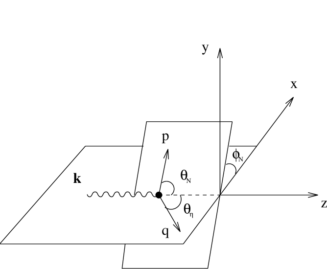
FIG. 4.: The coordinate system for the quasifree reaction $A(\gamma,\eta N)B$.

FIG. 5.: The energy dependence of the $\eta$ optical potential parameter $b$ for two different models of the $\eta N$ t-matrix. See Sec. III D for the discussion of DW1 and DW2.

FIG. 6.: Effects of distortions in the coincidence cross section and the photon asymmetry for $A(\gamma,\eta p),\;p_{3/2}$ at $E_{\gamma}$=750 MeV, $\theta_{\eta}=20^{0}$ and $\theta_{p}=15^{0}$. The dashed line is the plane wave calculation, the solid line is with $\eta$ distorted by the model DW1 while the proton is kept as plane wave, and the dot-dashed line is with $p$ distorted while $\eta$ is kept as plane wave.

FIG. 7.: Effects of the $\eta$-nucleus potential as a function of eta angle for plane wave, full DW1, and DW1 with real part turned off.

FIG. 8.: Effects of medium modifications to the $S_{11}(1535)$ resonance are shown by changing its bare mass by 3%. The reaction is ${}^{12}C(\gamma,\eta p)^{11}B_{g.s.}$ at $T_{\eta}$=100 MeV, $\theta_{\eta}=20^{0}$ and $\theta_{p}=20^{0}$.

FIG. 9.: Same as in Fig. 8, except for $D_{13}(1520)$.

FIG. 10.: Eta energy dependence of the inclusive cross section $d^{2}\sigma/dT_{\eta}d\Omega_{\eta}$ on ${}^{12}C$ and ${}^{40}Ca$ calculated in the plane wave (PW) and the two different $\eta$-nucleus potentials DW1 and DW2.

FIG. 11.: Same as in Fig. 10, but for the eta angular dependence.

FIG. 12.: Comparison of our calculations with the Mainz data [12] for the inclusive cross section $d\sigma/dT_{\eta}$ on ${}^{12}C$ and ${}^{40}Ca$.

FIG. 13.: Comparison of our calculations with the Mainz data [12] for the inclusive cross section $d\sigma/d\theta_{\eta}$ on ${}^{12}C$ and ${}^{40}Ca$.

FIG. 14.: Comparison of our calculations with the Mainz data for the total cross section on ${}^{12}C$ and ${}^{40}Ca$.