PAIRING CORRELATIONS BEYOND THE MEAN FIELD
Abstract
We discuss dynamical pairing correlations in the context of configuration mixing of projected self-consistent mean-field states, and the origin of a divergence that might appear when such calculations are done using an energy functional in the spirit of a naive generalized density functional theory.
1 Introduction
Self-consistent mean-field models are one of the standard approaches in nuclear structure theory, see Ref.[1] for a recent review. For heavy nuclei, they are the only microscopic method that can be systematically applied on a large scale.
Over the last few years, we were involved in the development of a method, that adds long-range correlations to self-consistent mean-field by projection after variation and variational configuration mixing within the generator coordinate method (GCM). A pedagogical introduction to our method is given in Ref.[2], we will sketch some of our recent work on those aspects of this method that concern the treatment of pairing correlations.
2 Theoretical framework
2.1 Self-consistent mean-field with pairing
For an introduction into the treatment of pairing correlations in a HFB framework, see for example[3, 4, 5] and references given therein. We will give only those details that are relevant for the further discussion.
All results given below were obtained with the effective Skyrme interaction SLy4[6] and a density-dependent pairing interaction with a soft cutoff at 5 MeV above and below the Fermi energy as described in Ref.[7]. The HFB equations are solved using the two-basis method introduced in Ref.[8]. All we need to know about an HFB state in what follows is that in its canonical basis it is given by
| (1) |
in terms of occupation probabilities and creation and annihilation operators.
HFB states are not eigenstates of the particle-number operator. In condensed matter, for which HFB theory was originally designed, this is not much of a problem, as the number of particles is usually huge. In nuclear physics, where the particle number is quite small, this causes two problems: On the one hand, the standard HFB treatment artificially breaks down when the density of single-particle levels around the Fermi energy is below a critical value, leading to a HF state without pairing correlations. On the other hand, a HFB state mixes the wave functions of different nuclei as it is spread in particle-number space, with a width that is proportional to the dispersion of the particle number[9].
3 Particle-number projection
variation after projection (VAP)[10] provides a rigorous solution to both problems. For various mainly technical reasons, however, this approach is not yet widely used (see[11] for an exception). We use a different approach instead, that was first outlined in Ref.[12]. In a first step, we complement the HFB equation with the Lipkin-Nogami (LN) method, that provides a numerically simple approximation to projection before variation, see Ref.[8] and references given therein for details. The LN procedure enforces the presence of pairing correlations also in the weak pairing regime at small level density. The LN method gives a correction to the total energy whose quality has been repeatedly questioned. We do not make use of the correction term, but project in a second step on exact eigenstates of the particle-number operator , with eigenvalue , applying the particle-number projection operator
| (2) |
The operator rotates the HFB state in a gauge space
| (3) |
while is a weight function. For states with even particle number the integration interval can be reduced to . We discretize the integrals over the gauge angle with a simple -point trapezoidal formula
| (4) |
As was shown by Fomenko[13], this simple scheme eliminates exactly all components from an HFB state which differ from the desired particle number by up to particles. Although the spread of the near-Gaussian distribution of particle numbers is large in comparison with respect to the constrained value, it is small enough that already small values of , ranging from 5 in light nuclei to 13 in heavy ones, are sufficient for the numerical convergence of the integrals over .
In practice, we constrain the HFB states in the mean-field calculations to the same (integer) particle number that we project on afterwards. This is, however, not a necessary condition. In a projection-before-variation approach, the particle number of the intrinsic state has no physical meaning, and will usually take a non-integer value close to, but not identical with, the particle number projected on[9, 10].
We address here only HFB states with pairing correlations among particles of the same isospin. In this case, the nuclear HFB state is the direct product of separate HFB states for protons and neutrons, respectively, which are separately projected afterwards on the number of the respective particle species.
3.1 Variational configuration mixing
In a mean-field calculation, one often encounters a situation where the total binding energy (mean field or projected) varies only slowly with a collective degree of freedom. In such a case, it can be expected that the nuclear wave function is widely spread around the mean-field minimum, which is beyond the scope of (projected) mean-field theory. These fluctuations around a single state can be incorporated within the generator coordinate method (GCM). The mixed projected many-body state is set-up as a coherent superposition of projected mean-field states which differ in one or several collective coordinates
| (5) |
The weight function is determined from the stationarity of the GCM ground state, which leads to the Hill-Wheeler-Griffin equation[14]
| (6) |
that gives a correlated ground state, and, in addition, a spectrum of excited states from orthogonalization to the ground state. The weight functions are not orthonormal. A set of orthonormal collective wave functions in the basis of the states is obtained from a transformation involving the square root of the norm kernel[15]. It has to be noted that projection is in fact a special case of the GCM, where degenerate states are mixed. The generators of the group involved define the collective path, and the weight functions are determined by the restored symmetry.
For a state which would result from the mixing of different unprojected mean-field states, the mean particle number will not not be equal to the particle number of the original mean-field states anymore. Projection on particle-number, as done here, eliminates this problem, otherwise a constraint on the particle number has to be added to the Hill-Wheeler-Griffin equation (6), see, for example, Ref.[15].
The technical challenges of a configuration-mixing calculation come from the non-diagonal kernels of different mean-field states, which are evaluated with a generalized Wick theorem[16, 17]. We represent the single-particle states on a 3-dimensional mesh in coordinate space using a Lagrange mesh technique[18]. As a consequence, the two sets of single-particle states representing the intrinsic HFB states entering the kernels are usually not equivalent, which has to be carefully taken into account[15, 19].
We usually combine the techniques presented above with a projection on angular momentum[19] that will not be discussed here. Applications are published in Refs.[20, 21, 22, 23, 24, 25, 26]. Similar methods, but without particle-number projection, have been set up using the Gogny force[27] and relativistic Lagrangians[28].
For the sake of simple notation, we have introduced the GCM using a many-body Hamiltonian . All the methods just mentioned, however, have in common that they are not based on a Hamiltonian, but an energy functional to calculate the binding energy. The necessary generalization will be sketched in section 5 below.
4 Dynamical pairing correlations
There is fundamental problem with projection after variation as performed here: it cannot be expected that the projection of the mean-field ground state (after variation) gives the minimum of the energy hyper-surface that is obtained by the projection of all possible mean-field states (which would be found by projection before variation). When projecting deformed mean-field states on angular-momentum, the intrinsic deformation of the mean-field ground state will indeed usually be different from the intrinsic deformation of the state giving the minimum of the projected energy curve, with the the exception of well-deformed heavy nuclei in the rare-earth, actinide, and transactinide regions.
In the context of angular-momentum projection, we overcome this problem to some extend by a minimization after projection (MAP), where we generate an energy curve of projected mean-field states with different intrinsic quadrupole deformation, whose minimum provides a first order approximation to projection before variation. When performing a GCM calculation of projected states, the spacing of points along this deformation energy curve does not need to be very dense, it even does not have to contain the actual minimum, as the variational projected GCM calculation of two (non-orthogonal) projected states around a minimum has the ability to (implicitely) construct this minimum, as the projected state representing the minimum has a non-zero overlap with the actually used states. As the projected GCM ground state also describes the energy gain from fluctuations around this minimum, its energy will be even below that of the minimum of the projected energy curve. It has to be stressed that the correlations from fluctuations around the projected state are outside the scope of projection before variation. As a consequence, projection before variation does not per se give a better description of correlations beyond the mean field than a GCM of states projected after variation.
While this is a standard procedure in the context of angular-momentum projection, where a MAP is performed with respect to quadrupole deformation, it has been rarely addressed in connection with particle-number projection. The most obvious degree of freedom to search for a minimum of a particle-number projected energy curve is the amount of pairing correlations contained in the (unprojected) intrinsic state. Using this degree of freedom in a projected GCM calculation is equivalent to including the ground-state correlations from pairing vibrations (see Refs.[4] for an overview and Refs.[29, 30] for early GCM calculations using schematic models). Exploratory studies along these lines within the context of realistic mean-field models are presented in Refs.[31, 32]. They do, however, not involve projection on angular momentum.
We will present here a similar study of the role of dynamical pairing correlations in 120Sn. First of all, we have to note that finding a suitable constraint on pairing correlations is not an easy task. The obvious choice in schematic models is the pairing gap obtained from a pairing force with constant matrix elements. This coordinate was, in fact, also used in Refs.[31, 32]. It has, however, some serious drawbacks as this pairing force leads to unrealistic asymptotics of the HFB state at large distances from the nucleus[5]. Constraints on other observables that measure pairing correlations pose similar problems even when used with a realistic pairing interaction, or they introduce ambiguities on how to put them into the variational equations[33]. The situation is similar to a constraint on a multipole moment of the density distribution of order used to generate an energy surface as a function of deformation. Such a constraint has always to be damped at large distances from the nucleus, as it introduces along some direction a contribution to the constrained single-particle potential that diverges as .
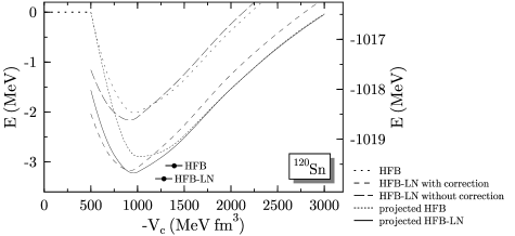
A not completely satisfactory, but well working constraint on the amount of pairing correlations is provided by the strength of the pairing force. A calculation is done in two steps: First, the HFB or HFB-LN equations are solved using a ”generating pairing strength” . Then, in a second step, the energy of each HFB state is re-calculated without iterating the HFB equations using the realistic pairing strength MeV fm3, either with or without projection. In a third step, the projected HFB states can be mixed within the GCM. Only the pairing strength of the neutrons is changed. For protons, we always use MeV fm3, and the same method as for the decription of the neutrons; in the case of pure HFB this means that the proton pairing breaks down. An example of such a calculation is shown in Fig. 1. The most remarkable findings are
1) The HFB equations without LN corrections break down to HF at values of the pairing strength around MeV fm3. For those states, our formalism cannot introduce pairing correlations beyond the mean-field. Just above the transition from an unpaired to a paired system, the energy gain from projection rises very rapidly up to about the corresponding to the minimum of the energy curve (which differes on the order of 10 from ), and decreases more slowly afterwards. This is analogue to what is found in the angular-momentum projection of quadrupole deformed states around a spherical configuration.
2) There are obvious differences between HFB and HFB-LN energy curves, both on the mean-field level and projected, for small generating pairing strength MeV fm3, which is indeed in the regime of the physical pairing strength. In the strong pairing regime at larger values of , the energy curves obtained from projection of the HFB and HFB-LN states are nearly identical. The remaining difference might be attributed to the presence of proton pairing correlations in the HFB-LN case, while they are absent for HFB.
3) The LN correction overestimates the energy gain from projection at small generating pairing strength, and underestimates it in the strong pairing regime.
4) The additional energy gain from the GCM of projected states is quite small, around 100 keV when starting with HFB-LN states, and about 200 keV for pure HFB states. The unphysical breakdown of HFB in the weak pairing regime leads to a smaller binding energy at the minimum of the projected energy curve, and gives a potential energy surface that is stiffer than the HFB-LN one for small . This leads to a GCM ground state from projected HFB that is less bound than the GCM gound state from projected HFB-LN. This also pushes the GCM ground state wave function from projected HFB to larger values of than the one from projected HFB-LN, as seen from the larger average generating pairing strength in the projected HFB case.
This calculation, of course, scratches only on the surface of the importance of dynamical pairing correlations. The question of better constraints on pairing correlations, systematics, excited states, and the coupling with deformation modes will be addressed elsewhere.
5 The divergence in particle-number projection
5.1 General features
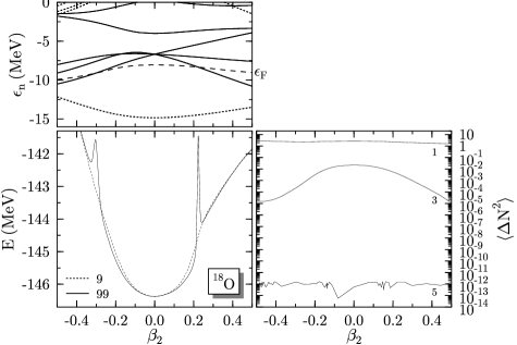
It has been noticed for a long time that the particle-number projected energy might exhibit divergences[34, 35] when a single-particle level crosses the Fermi energy and has the occupation . More recently, it was pointed out by Stoitsov et al.[36], that in addition to the divergence there appears a finite step in the projected energy when passing this situation as a function of a constraint. An example is given in Fig. 2, where two clear divergences appear when a fine discretization of the integral over gauge angles, Eq. (4), is used. The steps are also hinted, with the binding energy changing on both sides from a lower curve around sphericity to a higher lying curve when passing the divergence.
First of all, it has to be stressed that the binding energy is the only observable that shows an anomaly when a single-particle level crosses the Fermi energy. Neither the overlap, nor any observable calculated from any -body operator shows an unusual behaviour. This is examplified in Fig. 2 by the dispersion of the particle number, a two-body operator that also provides a measure for the numerical quality of projection. For a small system like 18O, the integrals over gauge angles are already numerically converged for discretization points. The only exception is the binding energy. However, an extremely huge number of discretization points is needed to see the divergence develop in 18O (and even more for heavier nuclei), which is one of the reasons why the divergence often remains undetected. The other reason is that it is very unlikely that one of the discrete points used to calculate a potential energy surface hits the narrow region where the divergence appears. This is different when performing projection before variation, where the variation will detect the divergences more easily[36].
The appearance of a divergence for the binding energy, but no other observable is related to the the particular definition of the binding energy in our method: the energy is calculated from an energy density functional, while everything else is, for the moment at least, calculated as the expectation value of an operator.
To understand the origin of the divergence, we have to look into the definition and evaluation of the energy functional. For the sake of simple notation and a transparent argument, we will restrict ourselves here to a toy model with one kind of particles only, and a two-body interaction. The additional complications introduced by density dependencies as needed in realistic energy functionals will be discussed elsewhere[37]. The further generalization to a system composed of protons and neutrons is then straightforward. All expressions given below are evaluated in the canonical basis, as this basis will turn out to be the only basis in which the origin of the divergence can be clearly identified and analyzed.
5.2 The Hamiltonian case
As a reference, for which everything is properly defined and no problem occurs, we will use the energy obtained from a two-body force. At the HFB level, one has
The contractions are the usual density matrix and pair tensor in the canonical basis
| (8) | |||||
| (9) | |||||
| (10) |
Unlike in papers on standard HFB theory we distinguish already here between two different pair tensors, as they generalize differently for particle-number projected HFB states. Unless necessary, we will not specify the kinetic energy in what follows. It is given by a one-body operator, always evaluated as such from whatever the left and right many-body states might be, and free of any divergence problems. The generalization of to particle-number projected states is straightforward
| (11) |
with . The relevant piece is the calculation of the Hamiltonian kernel Although for particle-number projection the Hamiltonian kernel can – in principle – be evaluated using the standard Wick theorem, it is much more convenient to apply a generalized Wick theorem[16, 17]
| (12) | |||||
The basic contractions are given by
| (13) | |||||
| (14) | |||||
| (15) |
and the norm kernel by
| (16) |
5.3 The EDF case
In the case of general energy density functional (EDF) in the spirit of a Kohn-Sham approach with pairing, the energy is given by
| (17) |
where is the kinetic energy, the energy of the particle-hole interaction, and the energy from the particle-particle (pairing) interaction. The only restriction that we impose on the energy functional for the moment is that it is bilinear in either the density matrix or the pair tensor, which is done to keep the analogy with the Hamiltonian case. Then, the energy functional can always be described in terms of the kinetic energy and a double sum over not antisymmetrized two-body matrix elements and , different in the particle-hole
| (18) | |||||
This is the Kohn-Sham approach to an EDF[38], formally generalized to systems with pairing by Oliveira et al.[39], where the actual density (matrix) is calculated from an auxiliary independent quasi-particle state . Equation (18) might appear to be an unusual representation of an energy functional, but, for example, the interaction of a term bilinear in the local density, where is an arbitrary function and the coupling constant, translates as
| (19) | |||||
Similar expressions are obtained for any other bilinear contribution to an energy functional that does not have density-dependent coupling constant.
For the generalization of the energy functional to the case of particle-number projected states, the same generalized Wick theorem as above is used to define
| (20) |
where the Hamiltonian kernels are now given by
| (21) | |||||
The identification of the origin of the divergence proceeds as follows
1) As analyzed in detail by Anguiano et al.[35], the divergence appears for those terms in the energy that originate from the interaction of a particle with its conjugated partner
| (22) | |||||
For and , the denominator in the transition densities becomes zero. One of the two denominators is canceled by the same factor contained in , Eq. (16), while the other one causes the divergence[35].
2) It can be shown from very general arguments[37] that the Hamiltonian kernel should have a certain dependence on . The divergent contributions to (22) do not follow this rule. This shows that such terms are spurious even for .
3) In the case of a two-body Hamiltonian the divergence disappears when one identifies and . This can be used to combine the and factors such that they cancel the dangerous denominator[35].
4) The matrix elements of the kind might indeed have non-zero values in an EDF, which represent a spurious interaction of a particle with itself. They violate the exchange symmetry in a Fermionic systems (the Pauli principle), and lead to a spurious contribution to the total binding energy already on the mean-field level. The appearance of this so-called ”self-interaction” is a well-known annoyance of EDFs for electronic systems[40], but ignored in nuclear physics so far.
5) In the case of an EDF with pairing, there is an additional spurious ”self-pairing” interaction that originates from the scattering of a pair onto itself. The interaction energy from two isolated Fermions occupying pair-conjugated orbitals divided by the occupation of the pair should have the same value as if pairing correlations were not present[37]. Again, this is violated by a general EDF. The actual expression for the spurious self-pairing energy combines matrix elements and the occupation factors that weight them and will be given elsewhere[37].
6) The divergent contributions to Eq. (22) come from terms that represent self-interaction and self-pairing. By that, the projection adds a second level of spuriosity to these terms. Not the whole contribution from the self-interaction and self-pairing terms is divergent, though.
7) The self-interaction and self-pairing contribute to the total energy not only because the relevant matrix elements have spurious non-zero values, but also because they are multiplied with unphysical weights. When evaluating the Hamiltonian kernel (12) by commutating the creation and annihilation operators of the Hamiltonian with those setting up the HFB states until they hit the vacuum, it becomes clear that each pair of conjugated particles can be multiplied with one factor stemming from the rotated state to the right only, and that the possible combinations of and for a given will always be bilinear. Only when the Wick theorem is applied, one obtains terms which are of 4th order in and and quadratic in . The reason is that multiple contributions from the same particle or pair of particles are not excluded from the sum as the Wick theorem implicitely assumes that the matrix elements these terms multiply are zero or sum up to zero, so that they will not contribute anyway. In an EDF these matrix elements are not zero anymore, but the Wick theorem is still used.
One rigorous way to remove the spurious terms from an energy functional would be to remove all possible self-interactions in the total energy by excluding that the same summation index appears more than once in a contribution to Eq. (18) This was, in fact, already used by Hartree in his seminal paper on the Hartree method[41]. Or, alternatively, one sums up explicitely all the contributions where the same summation index appears two times or more often and subtracts this as a self-energy correction from the total energy[40]. This leads, however, to enourmous complications in the variational equations, particularly when extended to density-dependent interactions.
5.4 The origin of the finite step
As pointed out by Stoitsov et al.[36], there is also a finite step that appears when passing the divergence as a function of a collective coordinate. The analysis of its origin will be given elsewhere[37]. Let us just outline the main arguments: With the substitution , the integral over the real gauge angle in Eq. (2) can be transformed into an integral in the complex plane, that can be analyzed with the tools from function theory[36, 37]. In the Hamiltonian case, the integral has a pole at , which has an order of the number of particles below the Fermi energy. The residue of this pole is proportional to the projected energy. In a projected EDF framework, there are two changes to this scenario: First, there is an additional contribution to the pole at , this time from all particles, and second, there appear additional poles at along the imaginary axis, which also contribute for all particles below the Fermi energy. Both originate from the same terms as the divergence. The two additional contributions to the projected energy are huge (on the order of several hundered MeV for 18O), but of opposite sign and nearly, but not exactly, canceling each other. The step appears when one of the poles at enters or leaves the integration contour when the single-particle energy of the corresponding particle crosses the Fermi energy.
6 Further discussion
Density-dependent terms add further complications to the divergence, which we will not address here in detail. Let us just comment that, first, in a projected theory, the evaluation of a density-dependent term with non-integer power requires the evaluation of a (multivalued) root of a complex number, which leaves the Riemann sheet for choice. Second, when one expands the densities in the energy functional for density-dependent terms, and combines the resulting terms similar to Eq. (5.3), one finds again terms which contain more than just one factor originating from (one of them with a usually non-integer power), which again introduces an unphysical dependence on into the Hamiltonian kernel.
There are good and profound reasons to use different effective interactions in the particle-hole and particle-particle channels. The particle-hole and particle-particle channel of the effective interaction sum up different classes of diagrams[43], which inevitably leads to different expressions for the effective interaction in both channels. Short-range correlations are resummed into the functional providing the two channels with different density-dependent forms. On the other hand, the long-range correlations from large-amplitude fluctuations around the mean-field states are either neglected in a pure mean-field approach when they are assumed to be small, or otherwise described explicitely by projection and GCM-type configuration mixing. A correction that removes the divergent part and the finite step from the projected energy can be set-up when identifying the terms with an unphysical dependence on the gauge angle comparing the expressions obtained from the standard and generalized Wick theorem[37, 42].
While particle-number projection is the prominent example for the appearance of a divergence, similar divergences can be expected in any GCM calculation or projection on any other quantum number. As in these cases the mixed states have different canonical bases, the transition density matrix is usually not diagonal and the analysis is less obvious. The widely used collective Schrödinger equation and Bohr Hamiltonian that are set-up through a series of approximations (at some points including improvements) from exact configuration mixing cannot be expected to be free of problems stemming from the divergence either, although there they will be more difficult to identify.
7 Summary
First, we have examined for the example of 120Sn the effect of a minimization after particle-number projection and of GCM ground state correlations from pairing vibrations. For 120Sn, the effect is visible, but not enormous, and clearly smaller than the current uncertainties from the parameterization of the effective pairing interaction. This might be, however, different for other nuclei.
Second, we have examined the divergence that appears in particle-number projected EDF. As its origin we identify the spurious self-pairing contribution contained in all common energy functionals for self-consistent mean-field models. On the mean-field level, the self-pairing as such adds a small spurious contribution to the total binding energy, that is similar to, but smaller, than the usual spurious centre-of-mass or rotational energies from broken symmetries (in fact, together with the self-energy it is the spurious energy from violating the Pauli principle in approximate EDF approaches). When generalizing the EDF to particle number projection via the generalized Wick theorem, the self-pairing provides the Hamiltonian kernels with an unphysical dependence on the gauge angle, which ultimately leads to divergences and steps.
Acknowledgements
The authors thank K. Bennaceur D. Lacroix, and P.-H. Heenen for many fruitful discussions on the theoretical and numerical treatment of dynamical pairing correlations, and J. Dobaczewski, W. Nazarewicz, M. V. Stoitsov, and L. Robledo for many inspiring and clarifying discussions on the appearance and interpretation of, and the threat posed by, the divergence and step in particle-number projected EDF.
References
- [1] M. Bender, P.-H. Heenen, and P.-G. Reinhard, Rev. Mod. Phys. 75, 121 (2003).
- [2] M. Bender and P.-H. Heenen, Eur. Phys. J. A 25, s01 (2005) 519.
- [3] H. J. Mang, Phys. Rep. 18, 327 (1975).
- [4] P. Ring and P. Schuck, The Nuclear Many-Body Problem, Springer Verlag, New York, Heidelberg, Berlin, 438 (1980).
- [5] J. Dobaczewski, H. Flocard, J. Treiner, Nucl. Phys. 422, 103 (1984).
- [6] E. Chabanat, P. Bonche, P. Haensel, J. Meyer, and R. Schaeffer, Nucl. Phys. A635, 231 (1998); Nucl. Phys. A643, 441(E) (1998).
- [7] C. Rigollet, P. Bonche, H. Flocard, P.-H. Heenen, Phys. Rev. C 59, 3120 (1999).
- [8] B. Gall, P. Bonche, J. Dobaczewski, H. Flocard, and P.-H. Heenen, Z. Phys. A348, 183 (1994).
- [9] H. Flocard and N. Onishi, Ann. Phys. 254 (1997) 275.
- [10] J. A. Sheikh and P. Ring, Nucl. Phys. A665, 71 (2000).
- [11] M. V. Stoitsov, J. Dobaczewski, R. Kirchner, W. Nazarewicz, J. Terasaki, preprint nucl-th/0610061.
- [12] P.-H. Heenen, P. Bonche, J. Dobaczewski, H. Flocard, Nucl. Phys. A561, 367 (1993).
- [13] V. N. Fomenko, J. Phys. (G.B) A 3, 8 (1970).
-
[14]
D. L. Hill and J. A. Wheeler,
Phys. Rev. 89, 1106 (1953);
J. J. Griffin and J. A. Wheeler, Phys. Rev. 108, 311 (1957). - [15] P. Bonche, J. Dobaczewski, H. Flocard, P.-H. Heenen and J. Meyer, Nucl. Phys. A510, 466 (1990).
- [16] N. Onishi and S. Yoshida, Nucl. Phys. 80, 367 (1966).
- [17] R. Balian and E. Brézin, Il Nuovo Cimento, B 64, 37 (1969).
- [18] D. Baye and P.-H. Heenen, J. Phys. A19, 2041 (1986).
- [19] A. Valor, P.-H. Heenen, P. Bonche, Nucl. Phys. A671, 145 (2000).
- [20] M. Bender and P.-H. Heenen, Nucl. Phys. A713, 390 (2003).
- [21] M. Bender, H. Flocard, P.-H. Heenen, Phys. Rev. C 68, 044321 (2003).
- [22] T. Duguet, M. Bender, P. Bonche, P.-H. Heenen, Phys. Lett. B559, 201 (2003).
- [23] M. Bender, P. Bonche, T. Duguet, P.-H. Heenen, Phys. Rev. C 69, 064303 (2004).
- [24] M. Bender, P.-H. Heenen, P. Bonche, Phys. Rev. C 70, 054304 (2004).
-
[25]
M. Bender, G. F. Bertsch, P.-H. Heenen,
Phys. Rev. Lett. 94, 102503 (2005);
Phys. Rev. C 73, 034322 (2006). - [26] M. Bender, P. Bonche, P.-H. Heenen, Phys. Rev. C 74, 024312 (2006).
- [27] R. R. Rodriguez-Guzman, J. L. Egido, and L. M. Robledo, Phys. Rev. C 62, 054319 (2002); J. L. Egido, L.M. Robledo, Lecture Notes in Physics No. 641 (Springer, Berlin, 2004), p. 269.
- [28] T. Nikšić, D. Vretenar, and P. Ring, Phys. Rev. C 73, 034308 (2006).
- [29] G. Ripka and R. Padjen, Nucl. Phys. A132, 489 (1969).
- [30] A. Faessler F. Grümmer, A. Plastino, F. Krmpotic, Nucl. Phys. A217, 420 (1973).
- [31] J. Meyer, P. Bonche, J. Dobaczewski, H. Flocard, P.-H. Heenen, Nucl. Phys. A533, 307 (1991).
- [32] P.-H. Heenen, A. Valor, M. Bender, P. Bonche, H. Flocard Eur. Phys. J. A11, 393 (2001) .
- [33] M. Bender, K. Bennaceur, and T. Duguet, unpublished.
- [34] F. Dönau, Phys. Rev. C 58, 872 (1998).
- [35] M. Anguiano, J. L. Egido, and L. M. Robledo, Nucl. Phys. A696, 467 (2001).
- [36] J. Dobaczewski, W. Nazarewicz, P.-G. Reinhard, and M. V. Stoitsov, in preparation.
- [37] M. Bender and T. Duguet, in preparation.
-
[38]
W. Kohn and L. J. Sham,
Phys. Rev. 137, A1697 (1964);
W. Kohn, Rev. Mod. Phys. 71, 1253 (1998). - [39] L. N. Oliveira, E. K. U. Gross, and W. Kohn, Phys. Rev. Lett. 60, 2430 (1988).
- [40] J. P. Perdew and A. Zunger, Phys. Rev. B23, 5048 (1981).
- [41] D. R. Hartree, Proc. Cambridge Philos. Soc., Vol. 1928, 89 (1928).
- [42] D. Lacroix, T. Duguet and M. Bender , in preparation.
- [43] E. M. Henley and L. Wilets, Phys. Rev. 133, B 1118 (1964).