An equations-of-motion approach to quantum mechanics:
application to a model phase transition

Abstract

We present a generalized equations-of-motion method that efficiently calculates energy spectra and matrix elements for algebraic models. The method is applied to a 5-dimensional quartic oscillator that exhibits a quantum phase transition between vibrational and rotational phases. For certain parameters, $10\times 10$ matrices give better results than obtained by diagonalising 1000 by 1000 matrices.

Equations-of-motion methods Sawada ; Kerman ; KK ; RowRMP offer an alternative to diagonalization of a Hamiltonian to determine the properties of a quantal system. We consider systems with a Hamiltonian expressed in terms of a Lie algebra of observables, $\mathfrak{g}$. For a finite-dimensional irreducible representation (finite irrep) of $\mathfrak{g}$, both approaches give the same results. However, they become inequivalent when approximations are necessary. For example, diagonalizing the Hamiltonian for a system of $n$ coupled harmonic oscillators, in a basis of uncoupled harmonic oscillator states, gives results that become precise (to within computational errors) in an infinite limit whereas an equations-of-motion approach, as given by the standard random phase approximation (RPA), is already precise in a $2n$-dimensional space.

Problems of interest are ones for which an expansion of the low-energy eigenstates of the Hamiltonian, in a given ordered basis for the Hilbert space, converges slowly. For example, the low-energy states of strongly-deformed rotational nuclei are dominated by components from higher shells in contrast to the low-energy states of a near-spherical nucleus which may be dominated by the valence-shell states of a spherical harmonic-oscillator shell-model basis NShapes . In such a situation, diagonalization of the Hamiltonian in a spherical shell-model basis is unlikely to give reliable results.

The proposed approach avoids the preliminary stage of defining basis states and proceeds directly to the determination of a matrix representation of the algebra of observables in which the Hamiltonian is diagonal. The approach has its origins in three previous developments: a variational technique Ros ; RR for computing the irreps of potentially difficult Lie algebras; the double-commutator equations-of-motion formalism RowRMP ; and the equations-of-motion method of Kerman and Klein KK ; LiK . Thus, we refer to it as the RRKK equations-of-motion method.

Consider a Hamiltonian $\hat{H}$ that is a polynomial in the elements $\{\hat{X}_{\nu}\}$ of a Lie algebra $\mathfrak{g}$ of observables with commutation relations $[\hat{X}_{\mu},\hat{X}_{\nu}]=\sum_{\sigma}C^{\sigma}_{\mu\nu}\,\hat{X}_{\sigma}$. We refer to $\mathfrak{g}$ as a spectrum generating algebra (SGA), For each $\hat{X}_{\nu}\in\mathfrak{g}$, define $\hat{\cal H}_{\nu}:=[\hat{H},\hat{X}_{\nu}]$. The objective is to determine a unitary irrep in which each observable $\hat{X}_{\nu}$ is represented by a matrix $X(\nu)$, with elements

$$X_{ij}(\nu):=\langle i|\hat{X}_{\nu}|j\rangle,$$ (1)

to be determined along with energy differences $\{E_{i}-E_{j}\}$, such that the sets of equations

$$f_{ij}(\mu,\nu):=\langle i|[\hat{X}_{\mu},\hat{X}_{\nu}]|j\rangle-\sum_{\sigma}C^{\sigma}_{\mu\nu}\langle i|\hat{X}_{\sigma}|j\rangle=0,\quad$$ (2)

$$f_{ij}(\nu):=\langle i|{\cal H}_{\nu}(\hat{X})|j\rangle-(E_{i}-E_{j})\langle i|\hat{X}_{\nu}|j\rangle=0,\quad$$ (3)

are satisfied. In general, it will also be necessary to include additional equations to ensure that the representation is the one desired. For example, if the Lie algebra has Casimir invariants, $\hat{C}_{n}(\mathfrak{g})$, equations can be included to require that they are represented by the appropriate multiples of the unit matrix, $c_{n}I$.

Let $F$, a so-called objective function, be defined for a finite irrep of dimension $N$ as the sum of squares

$$F = \sum_{i,j}^{N}\Big{[}\sum_{\mu\nu}\big{|}f_{ij}(\mu,\nu)\big{|}^{2}+\sum_{\nu}\big{|}f_{ij}(\nu)\big{|}^{2}$$ (5)

$$+\sum_{n}\big{|}\langle i|\hat{C}_{n}(\mathfrak{g})-c_{n}|j\rangle\big{|}^{2}\Big{]}.$$

$F$ cannot be negative and can only vanish when a precise solution to the system of equations has been obtained. Thus, for finite irreps, precise solutions to the above equations are obtained by minimization of $F$ as a function of the unknown matrix elements of the observables and the energy differences. If needed, the Hamiltonian matrix can also be evaluated as a polynomial in the $\{X(\nu)\}$ matrices to determine the ground-state energy.

The challenge is to obtain accurate solutions for finite submatrices of the observables, corresponding to a subset of lowest-energy eigenstates, when the irrep is infinite. Recall that a differential equation defined over the positive half of the real line, $0<r<\infty$, can be solved precisely over a finite interval $0<r\leq R$, if one knows the boundary conditions at $R$. Similarly, when infinite dimensional matrices $\{X(\mu)\}$ are truncated to finite dimensions, their outer rows and columns provide boundaries and their entries can be adjusted to give accurate results for the matrices they enclose.

The concern with boundary conditions in the equations-of-motion approach arises because, the equations of motion for a subset of matrix elements $\{X_{ij}(\nu);1\leq i,j\leq N\}$, involve the commutation relations

$$f_{ij}(\mu,\nu)=\sum_{k=1}^{\infty}\big{[}X_{ik}(\mu)X_{kj}(\nu)-X_{ik}(\nu)X_{kj}(\mu)\big{]}$$ (6)

and, hence, $X_{ik}(\mu)$ matrix elements with $k>N$.

This concern can be resolved as follows: because the matrix elements connecting lowest-energy states are of most interest, we apply a weighting factor $w_{ij}=1/[(i+1)(j+1)]$ to the expressions that should vanish for an exact solution; i.e., redefine the objective function to be minimized as

$$F^{\prime} = \sum_{i,j}^{N}w^{2}_{ij}\Big{[}\sum_{\mu\nu}\big{|}f_{ij}(\mu,\nu)\big{|}^{2}+\sum_{\nu}\big{|}f_{ij}(\nu)\big{|}^{2}$$ (8)

$$+\sum_{n}\big{|}\langle i|C_{n}(\mathfrak{g})-c_{n}|j\rangle\big{|}^{2}\Big{]}.$$

We also make the approximation

$$f_{ij}(\mu,\nu)\approx\sum_{k=1}^{N+1}\big{[}X_{ik}(\mu)X_{kj}(\nu)-X_{ik}(\nu)X_{kj}(\mu)\big{]}$$ (9)

and corresponding approximations for the evaluation of $f_{ij}(\nu)$ and the matrix elements of Casimir invariants. Minimization of the objective function is then carried out iteratively starting from a first guess. Thus, a simple physical model of the system can be used to provide a (possibly inconsistent) first guess which can then be made accurate by the equations-of-motion method.

To illustrate, consider a Hamiltonian, of relevance in the nuclear collective model Diep ; TR ; RT ,

$$\hat{H}_{\alpha}=-\frac{1}{2M}\nabla^{2}+\frac{M}{2}[(1-2\alpha)\beta^{2}+\alpha\beta^{4}]$$ (10)

for an object in a five-dimensional Euclidean space; $\beta$ is a radial coordinate in harmonic oscillator units, $\nabla^{2}$ the Laplacian, and $M$ is a dimensionless mass parameter. Such a Hamiltonian is of general interest as a model of a system with two phases: when $\alpha<0.5$, the potential

$$V_{\alpha}(\beta)=\frac{M}{2}[(1-2\alpha)\beta^{2}+\alpha\beta^{4}]$$ (11)

has a spherical minimum (at $\beta_{0}=0$); and when $\alpha>0.5$, it has a minimum given by $\beta_{0}^{2}=(2\alpha-1)/2\alpha$. It is invariant under the group of SO(5) rotations in the five-dimensional space. Thus, its eigenfunctions are products of $\beta$ wave functions and SO(5) spherical harmonics. For a state of SO(5) angular momentum $v$, the $\beta$ wave function is an eigenfunction of the radial component of $\hat{H}_{\alpha}$

$$\hat{H}_{\alpha}^{(v)}=-\frac{1}{2M}\frac{d^{2}}{d\beta^{2}}+\frac{(v+1)(v+2)}{2M\beta^{2}}+\frac{M}{2}[(1-2\alpha)\beta^{2}+\alpha\beta^{4}].$$ (12)

This radial Hamiltonian can be expressed Row05 in terms of an su(1,1) Lie algebra spanned by

$$\begin{array}[]{c}\displaystyle\hat{X}_{1}^{(v)}=\frac{d^{2}}{d\beta^{2}}-\frac{(v+1)(v+2)}{\beta^{2}}\,,\\ \hat{X}_{2}^{(v)}=\beta^{2},\quad\displaystyle\hat{X}_{3}^{(v)}=1+2\beta\frac{d}{d\beta}\,.\end{array}$$ (13)

In terms of su(1,1) raising and lowering operators,

$$\begin{array}[]{c}\displaystyle\hat{S}^{(v)}_{0}=\frac{1}{4}\bigg{[}-\frac{\hat{X}^{(v)}_{1}}{M}+M\hat{X}^{(v)}_{2}\bigg{]},\\ \displaystyle\hat{S}^{(v)}_{\pm}=\frac{1}{4}\bigg{[}\frac{\hat{X}^{(v)}_{1}}{M}+M\hat{X}^{(v)}_{2}\mp\hat{X}^{(v)}_{3}\bigg{]}\end{array}$$ (14)

which satisfy the commutation relations

$$\big{[}\hat{S}^{(v)}_{0},\hat{S}^{(v)}_{\pm}\big{]}=\pm\hat{S}^{(v)}_{\pm},\quad\big{[}\hat{S}^{(v)}_{-},\hat{S}^{(v)}_{+}\big{]}=2\hat{S}^{(v)}_{0},\quad$$ (15)

we obtain

$$\hat{H}^{(v)}_{\alpha} = 2(1-\alpha)\hat{S}^{(v)}_{0}-\alpha\left(\hat{S}^{(v)}_{+}+\hat{S}^{(v)}_{-}\right)$$ (16)

$$+\frac{\alpha}{2M}\left(2\hat{S}^{(v)}_{0}+\hat{S}^{(v)}_{+}+\hat{S}^{(v)}_{-}\right)^{2}.$$

For states of SO(5) angular momentum $v$, the su(1,1) Casimir invariant

$$\hat{C}_{v}({\rm su(1,1)})=\hat{S}_{0}(\hat{S}_{0}-1)-\hat{S}_{+}\hat{S}_{-}$$ (17)

takes the value

$$c_{v}=\textstyle\frac{1}{4}\big{(}v+\frac{5}{2}\big{)}\big{(}v+\frac{1}{2}\big{)}.$$ (18)

To start the minimization process, a first guess is provided for small $\alpha$ (compared to the critical value $\alpha_{c}=0.5$) by the RPA that retains only quadratic terms in a Taylor expansion of the Hamiltonian. In the present example, this amounts to dropping the quartic term in the potential and making the approximation

$$V_{\alpha}(\beta)\approx\frac{M}{2}(1-2\alpha)\beta^{2}.$$ (19)

For large $\alpha$, the Hamiltonian $\hat{H}^{(v)}_{\alpha}$ can be approximated by its asymptotic limit, obtained from a Taylor expansion of $V_{\alpha}(\beta)$ about its minimum $V_{\alpha}(\beta_{0})$,

$$\hat{H}^{(v)}_{\rm as}=-\frac{1}{2M}\frac{d^{2}}{d\beta^{2}}+\ \frac{(v+1)(v+2)}{2M\beta_{0}^{2}}+\frac{M\omega^{2}}{2}(\beta-\beta_{0})^{2}.$$ (20)

This approximation becomes precise as $\alpha\to\infty$ or, for $\alpha>0.5$, as $M\to\infty$. The physical content of these two limiting solutions is clear. The first is that of a spherical harmonic vibrator. The second is that of a rotor in a five-dimensional space, with moment of inertia $M\beta_{0}^{2}$, coupled to a harmonic radial $\beta$-vibrator. Thus, with the substitution

$$\displaystyle\beta-\beta_{0}=\frac{1}{\sqrt{2M\omega}}(c^{\dagger}+c),$$ (21)

$$\displaystyle\frac{d}{d\beta}=\sqrt{\frac{M\omega}{2}}\,(c-c^{\dagger}).\,$$ (22)

the asymptotic Hamiltonian is given by

$$\hat{H}^{(v)}_{\rm as}=\omega(c^{\dagger}c+\textstyle{1\over 2})+\displaystyle\frac{(v+1)(v+2)}{2M\beta_{0}^{2}}.$$ (23)

Corresponding approximations for the su(1,1) operators are given by

$$\hat{X}_{1}=\displaystyle\frac{M\omega}{2}(c^{\dagger}c^{\dagger}+cc-c^{\dagger}c-cc^{\dagger})-\frac{(v\!+\!1)(v\!+\!2)}{\beta_{0}^{2}},$$ (24)

$$\hat{X}_{2}=\displaystyle\big{[}\beta_{0}+\!\frac{1}{\sqrt{2M\omega}}(c^{\dagger}+c)\big{]}\big{[}\beta_{0}+\!\frac{1}{\sqrt{2M\omega}}(c^{\dagger}+c)\big{]},$$ (25)

$$\hat{X}_{3}=\displaystyle 1+\big{[}\sqrt{2M\omega}\,\beta_{0}+(c^{\dagger}+c)\big{]}(c-c^{\dagger}).$$ (26)

These approximations, provide first guesses for $\alpha<0.5-\delta$ and $\alpha>0.5+\delta$ respectively. In the transition region, $|\alpha-0.5|\leq\delta$, one can proceed in steps using the results of one calculation as a first guess for the next.

Before presenting results, it is instructive to consider what would be required for accurate results by diagonalization methods. Fig. 1 shows the expansion coefficients for the $v=0$ ground state in a harmonic oscillator basis for $\alpha=2,10$ and $M=2000$.

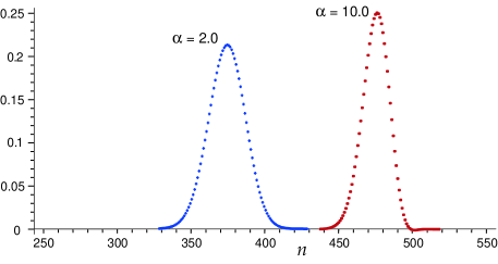
Figure 1: Expansion coefficients for an expansion of the ground states of $\hat{H}(\alpha)$ with $\alpha=2,10$ and $M=2000$ in the spherical $(\alpha=0)$ harmonic oscillator basis.

The figure suggests that at least 420 basis states, for $\alpha=2.0$, and 510 basis states, for $\alpha=10.0$, would be needed for the ground-state wave function. More basis states would be required for excited states. However, because the equations-of-motion approach does not use a predetermined basis, it is possible to obtain accurate values for energy eigenvalues for low-energy states and matrix elements in a basis of energy eigenstates with much smaller matrices.

The number of unknowns to be determined is reduced by exploiting the fact that $\hat{S}^{(v)}_{0}$ is self-adjoint and $(\hat{S}^{(v)}_{+})^{{\dagger}}=\hat{S}^{(v)}_{-}$. The lowest energy level was set to zero and the energies $\{E_{i}\}$ of excited states regarded as unknowns. For the calculations reported here, the function, $F^{\prime}$ was evaluated using Maple and minimized using the ‘lsqnonlin’ algorithm in Matlab. Results obtained with $N=10$ and a range of $\alpha$ and $M$ values are shown below. Minimization of $F^{\prime}$ determines 197 unknowns and approximately satisfies 500 equations. The values of $m$ for which the entries of the $m\times m$ submatrices are accurate to better than 8 significant figures are listed in Table 1. Numerically precise reference results were obtained by diagonalizing very large Hamiltonian matrices in the spherical harmonic basis.

Table 1: Values of $m$ for the $m\times m$ submatrices, obtained with $N=10$ for $v=2$, whose elements are accurate to at least 8 significant figures. The numbers in brackets are the estimated sizes of the Hamiltonian matrix required to achieve similar accuracy by diagonalization.

$\alpha$	$M=5$	$M=50$	$M=500$	$M=5000$
0.2	$m=$7 (25)	8 (15)	9 (20)	9 (20)
0.5	7 (30)	7 (20)	7 (45)	7(95)
0.7	7 (30)	6 (20)	6 (75)	7 (490)
1.0	7 (35)	5 (25)	7 (100)	8 (770)
2.0	7 (45)	5 (35)	7 (135)	8 (1065)
5.0	6 (65)	6 (60)	8 (175)	8 (1235)
10.0	6 (80)	6 (85)	8 (200)	8 (1295)
50.0	5 (150)	7 (180)	8 (310)	8 ($>$ 1500)

Typical computation times to obtain the result shown ranged from a few seconds to tens of seconds, achieving minimum values of $F^{\prime}\sim 10^{-20}$. A satisfying feature of the equations-of-motion approach is that its advantages over conventional diagonalization are most pronounced for large values of $M$ for which the diagonalization approach is most slowly convergent. Worst case scenarios for the equations-of-motion approach are when $M$ is small and $\alpha$ is large and when $M$ is large and $\alpha=0.5$. In the former case, the vibrational fluctuations about the equilibrium deformation are large, and in the latter case the critical point, $\alpha=0.5$, is highly singular. Even though the time taken to reach a minimum in such situations may be long, the results are invariably accurate. It is also noteworthy that, in the absense of good starting guesses, it is always possible to progress in steps from previously found solutions.

For the present model, it so happens that the $\alpha=0.5$ results are among the easiest to obtain for any value of $M$. This is because of a critical point scaling symmetry RTR which means that if the results are known for one value of $M$ they can simply be inferred for any $M$. For example, the Hamiltonian at $\alpha=0.5$ can be expressed

$$\hat{H}_{0.5}=-\frac{1}{2M}\nabla^{2}+\frac{M}{4}\beta^{4}=\frac{1}{2M^{1/3}}\Big{[}-\bar{\nabla}^{2}+\frac{1}{2}\bar{\beta}^{4}\Big{]},$$ (27)

with $\tilde{\beta}=M^{1/3}\beta$. Thus, the energy-level spectrum of $\hat{H}_{0.5}$ is independent of $M$ to within an $M^{-1/3}$ scale factor.

Table 2 gives an indication of the accuracy obtainable, for states of interest, by equations-of-motion calculations.

Table 2: Comparison between exact excitation energies and values calculated from the equations of motion for $\alpha=2$, $v=2$, and $M=50$ for different values of $N$.

Exact	$N=4$	$N=6$	$N=10$
2.420379968671	2.420382	2.420379969	2.420379968671
4.799716618277	4.7999	4.7997167	4.799716618277
7.136170688911	7.01	7.136180	7.136170688912
9.427750466577	-	9.4280	9.42775046660
11.672330365421	-	11.48	11.672330368
13.867713374832	-	-	13.8677136
16.011789014165	-	-	16.01180
18.102896804066	-	-	18.1033
20.140619242614	-	-	20.152

It compares excitation energies for the Hamiltonian, $\hat{H}_{\alpha}$ with $\alpha=2$, $v=2$, and $M=50$, obtained for various subspace dimensions with those of precise calculations. Even a calculation with $N=4$ gives accurately the first excitation energy to better than one part in $10^{6}$. This numerical accuracy is sustained for calculated energies up to the $N-3$ level.

Table 3 shows the excitation energies obtained by the equations-of-motion method with $N=5$ for the lowest two states of each SO(5) angular momentum $v=0,\dots,5$ for $M=50$ and a range of values of $\alpha$. The results are precise to better than the level of precision shown.

Table 3: The lowest two energy levels ($n=0$,1) with SO(5) angular momentum $v=0,\dots,5$, relative to the ground state energy, computed by the equations-of-motion method with $M=50$ and $N=5$. The results agree with those obtained by precise calculations to at least the level of precision shown. Results of the asymptotic approximation (AS) are shown in the last column for $\alpha=10$.

$n\;\;\;\;v$	$\alpha=0$	$\alpha=0.5$	$\alpha=1$	$\alpha=10$	AS, $\alpha=10$
0    0	0	0	0	0	0
0    1	1	0.40223	0.08712	0.04254	0.04211
0    2	2	0.84184	0.21629	0.10634	0.10526
0    3	3	1.31343	0.38597	0.19140	0.18947
0    4	4	1.81319	0.59436	0.29769	0.29474
0    5	5	2.33829	0.83960	0.42521	0.42105
1    0	2	0.96133	1.35973	6.13301	6.17262
1    1	3	1.45802	1.46666	6.17646	6.21472
1    2	4	1.97813	1.62318	6.24161	6.27788
1    3	5	2.52043	1.82581	6.32847	6.36209
1    4	6	3.08360	2.07109	6.43701	6.46735
1    5	7	3.66642	2.35579	6.56723	6.59367

It is instructive to note that the domains in which the diagonalization and equations-of-motion are most successful tend to be complementary. Matrix diagonalization is often faster. However, it requires much larger matrices and substantial extra work to set up the initial matrices and interpret the results in a given basis. In contrast, the equations-of-motion method, directly computes the matrices of all observables in the physically relevant basis of energy eigenstates. The advantages of the equations-of-motion are most evident for states of $\alpha\gg 0.5$ and large $M$. This is when states are beginning to approach their asymptotic dynamical symmetry limits. For example, for $v=2$, $\alpha=50$, and $M=5000$, one can obtain all the spectroscopic properties of the $m=8$ lowest states in 93 s, using $N=10$. Similar accuracy was only achieved by diagonalizing larger than $1500\times 1500$ matrices and took 250 s on the same computer. If one adds in the time taken to compute the matrices of Hamiltonian and other observables in a predefined basis, the equations-of-motion method wins hands down in such a situation. These advantages of the RRKK approach are expected to be more pronounced for systems with many degrees of freedom but relatively simple SGA’s.

An attractive property of the RRKK approach is that it makes it possible to start from a simple approximation and make it precise. Thus, the RRKK equations are particularly relevant for the description of systems that exhibit quantum phase transitions with variation of parameters, as this letter demonstrates. A natural possibility is to start with a mean field description of a phase transition and, on either side of the critical point, to use the RRKK equations of motion to add the fluctuation contributions that are missing in the mean field treatment.

References

- (1) K. Sawada, Phys. Rev. 106, 372 (1957).
- (2) A.K. Kerman, Ann. Phys. 12, 300 (1961).
- (3) A.K. Kerman and A. Klein, Phys. Rev. 132, 1326 (1963).
- (4) D.J. Rowe, Rev. Mod. Phys. 40, 153 (1968); Nuclear Collective Motion, (Methuen, London, 1970).
- (5) J. Carvalho and D.J. Rowe, Nucl. Phys. A 548, 1 (1992); M. Jarrio, J.L. Wood and D.J. Rowe, Nucl. Phys. A 528, 409 (1991); C. Bahri and D.J. Rowe, Nucl. Phys. A 662, 125 (2000).
- (6) G. Rosensteel, Phys. Rev. C 41, 730 (1990).
- (7) G. Rosensteel and D.J. Rowe, Phys. Rev. C 67, 014303 (2003); Nucl. Phys. A759, 92 (2005).
- (8) C-T. Li, A. Klein, F. Krejs, Phys. Rev. D 12, 2311 (1975); A. Klein, P. Protopapas, in Contemporary Nuclear Shell Models eds. X-W. Pan, D.H. Feng, M. Vallières (Springer-Verlag, Berlin) 1997, p. 201.
- (9) A.E.L. Dieperink, O. Scholten, and F. Iachello, Phys. Rev. Lett. 44 (1980), 1747; A.E.L. Dieperink and O. Scholten, Nucl. Phys. A346, 125 (1980).
- (10) P.S. Turner and D.J. Rowe, Nucl. Phys. A 756, 333 (2005).
- (11) D.J. Rowe and P.S. Turner, Nucl. Phys. A 753, 333 (2005).
- (12) D.J. Rowe, J. of Phys. A: Math. Gen. 38 10181 (2005).
- (13) D.J. Rowe, P.S. Turner and G. Rosensteel, Phys. Rev. Lett. 93 232502 (2004).