Models for photo- and electro-production of K⁺
in view of new data

Abstract

Predictions of isobaric and Regge models are compared with the latest experimental data (Bonn, JLab) to select among the models those providing a satisfactory description of the data. Only the Saclay-Lyon (SLA) and MAID models are in a reasonable agreement with both photo- and electro-production data ranging up to about $E^{lab}_{\gamma}=2.5$ GeV. In this energy region the Regge model is suitable only for description of the electro-production data and the older models Adelseck-Saghai (AS1, AS2), Workman (W1,W2), and Adelseck-Bennhold (AB2) can reliably predict only the photo-production cross sections up to $E^{lab}_{\gamma}=1.5$ GeV. In the kinematic region of the E98-108 experiment on the electro-production, SLA, Adelseck-Wright (AW4), Regge and MAID models are expected to provide an appropriate description of the separated cross sections whereas the unseparated cross sections can be reasonably well predicted also by the AW3 and Williams-Ji-Cotanch (C4) models.

1 Introduction

The photo- and electro-production of kaons on the proton in the resonance region have been studied both experimentally and theoretically since the 1960s. Many data were collected on the kaon photo-production (Cornell, Cal Tech, Bonn, Tokyo, DESY, and Orsay, see [1]) but only a few experiments were carried-out on the electro-production (Harvard-Cornell, DESY, and Cambridge, see [2] and references therein). Simulated by the availability of new facilities with higher current or/and high duty factor and polarization capability (JLab, Bonn, Grenoble), more precise data on both reactions have been accumulated starting in the late of 1990s which renewed interest in the subject. Now various response functions are accessible and measured with a good level of precision. The latest experimental data, especially those from JLab [3, 4, 5] on the separated cross sections in the electro-production in the kinematic region where scarce data were formerly available, allow to perform more rigorous tests of theoretical models and in this way improve our understanding of the elementary process.

Numerous theoretical attempts have been made to describe the electro-magnetic production of kaons with $\Lambda$ in the final state. In the kinematic region, $E^{lab}_{\gamma}=0.91-2.5$ GeV, the isobaric models [1, 6, 7, 8, 9, 10, 11, 12] are of particular interest. In these models the amplitude is derived from an effective hadronic Lagrangian using the Feynman diagram technique in the tree level approximation. However, it has been shown that the new data on $\rm p(e,e^{\prime}K)\Lambda$ [3] can be equally well described by the Regge model [13] which is based on the idea of exchanges of families of the particles with particular quantum numbers in the t-channel. The Regge model was aimed mainly for higher energies ($E_{\gamma}^{lab}>4$ GeV) and small angles. However, the model was successfully applied to description of the electro-production data at the centre of mass energy $W=1.84$ GeV [13].

In the isobaric models the invariant amplitude gains contributions from the extended Born diagrams, in which the proton, $\Lambda$, $\Sigma^{0}$, and kaon are exchanged in the intermediate state, and the resonant diagrams which include exchanges of moderate mass (less than 2 GeV) nucleon, hyperon, and kaon resonances. Unfortunately, due to absence of a dominant exchanged baryon resonance in the process [14], in contrast with the pion and eta production, many of exchanged resonances have to be a priori assumed to contribute [1, 11] introducing a rather large number of free parameters in calculations, the appropriate coupling constants. The free parameters are determined by fitting the cross sections and polarizations to the experimental data which, however, provides a copious number of possible sets of parameters [1, 11]. This large number of models which describe the data equally well can be reduced implementing duality hypothesis, crossing symmetry, and SU(3) symmetry constrains.

According to duality principle most of the nucleon resonances exchanged in the s-channel, especially those with a high spin, can be mimic by the lowest-mass kaon poles K^∗ and K₁ in the t-channel [10, 11]. The crossing symmetry constraint requires that a realistic model must yield simultaneously a reasonable description of the radiative capture of K^- on the proton with the lambda in the final state, which is related to the $\gamma\rm p\longrightarrow\Lambda K^{+}$ via the crossing symmetry [10, 11]. The flavor SU(3) symmetry allows to relate the main coupling constants $g_{\rm K\Lambda N}$ and $g_{\rm K\Sigma N}$ to the better established one, $g_{\pi\rm NN}$. For the 20% breaking of the SU(3) symmetry the following limits can be obtained: $-4.4\leq g_{\rm K\Lambda N}/\sqrt{4\pi}\leq-3.0$ and $0.8\leq g_{\rm K\Sigma N}/\sqrt{4\pi}\leq 1.3$ [1, 11]. Analysis of data performed under different assumptions about duality, crossing and SU(3) symmetry [1, 6, 7, 8, 10, 11, 12] showed that a moderate number of resonances is sufficient to get a reasonable agreement with the experimental data.

The models discussed above assume point-like particles in the hadron vertexes to ensure the gauge invariance principle. Recently Haberzettl et al. [15, 16] introduced hadron form factors in the gauge-invariant way in an isobaric model which required addition of a contact term to compensate the gauge-violating part of the amplitude. The method was worked out recently by Davidson and Workman [17] and further used by Janssen et al. [18]. Taking into account the hadron form factors led to reducing of divergences at higher energies inherent to most of isobaric models and also to more realistic predictions for the isospin-symmetry related $\rm n(\gamma,K^{0})\Lambda$ channel [15].

Another simplification assumed by the models is neglecting a meson-baryon re-scattering in the final state which obviously leads to violation of unitarity. Interaction of hadrons in the final state was taking into account for the photo-production reaction by Feuster and Mosel [19] employing the K-matrix approximation. Enforcing unitarity dynamically was performed by Chiang et al. [20] who utilised the coupled-channel approach. In their analysis they concluded that inclusion of the $\pi$N system in the intermediate state is needed for a proper description of the $\gamma\rm p\longrightarrow\Lambda K^{+}$ reaction.

More elementary approaches to study the reaction mechanism of $\gamma\rm p\longrightarrow\Lambda K^{+}$ was performed in terms of quark degrees of freedom in Refs. [21, 22, 23]. These models being in a closer connection with QCD than those based on the hadron degrees of freedom, need a smaller number of parameters to describe the data. Moreover, the quark models assume explicitly an extended structure of the hadrons which was found to be important for a reasonable description of the photo-production data [22]. Other approach to the $\gamma\rm p\longrightarrow\Lambda K^{+}$ reaction based on the Chiral Perturbation Theory [24] is applicable to the threshold region only.

This paper is aimed to discuss existing isobaric and Regge models for the electro-magnetic production of K⁺ off the proton particularly in view of the new experimental data [3, 4, 5, 25]. We intend to pick up among the models those reliable in the kinematic region of the E98-108 experiment [5] for further comparison with the coming data. The experiment E98-108 which was carried out in Hall A at Jefferson Lab in 2001 and 2002 extends the present data on the separated cross sections of the $\rm p(e,e^{\prime}K)\Lambda$ reaction to higher energies and larger $Q^{2}$ ($Q^{2}=-q^{2}_{\gamma}$) providing very good quality data and consequently it can set stringent constraints on the models. In the next section we briefly outline the models. In the section 3 we discuss predictions of the models in comparison with the new data.

2 Models

In comparison performed here we adopted a set of isobaric models, which are sufficiently well described in literature to enable performing calculations, and the Regge model. We also adopted results of the model by Bennhold et al. utilising the “new isobar model (Dec 2000)” interactive code at the KAON-MAID Web-page [16]. Those, trivial, isobaric models which assume only the Born terms (AB1 [6] and AW1 [7]) were omitted from the analysis.

The isobaric models selected for the comparison can be grouped according to the reaction they were determined for:
 1. photo-production only: AB2 [6], AW2 [7], AS1, AS2 [1], W1 and W2 [8].
 2. electro-production only: AW3 [7].
 3. photo- and electro-production: AW4 [7], C3 [9], C4(WJC) [10], SL [11] and SLA [12].

The models in the first group have to be extended for $\rm p(e,e^{\prime}K)\Lambda$ assuming a particular prescription for the electro-magnetic form factors of the mesons and baryons. Results of these models for the electro-production, therefore, depends to some extent on an ansatz we made for the electro-magnetic form factors and in this limited sense the models are predictive. In this analysis we used phenomenological prescriptions [27] fixed by the electron scattering. The meson form factors were supposed to be of the monopole form with $m_{V}=0.77$ GeV for all mesons whereas the dipole form, with $G_{E}(Q^{2})=(1+Q^{2}/m_{V}^{2})^{-2}$ and $m_{V}=0.84$ GeV, was used for all baryons.

Unfortunately, there are several models, AW3, AW4, C3, and C4, which were not sufficiently well commented in the original paper and for which either a definition or a form of the electro-magnetic form factors is not clear. In that cases we tried several possibilities to introduce the form factors. Finally we have chosen those which provide the best agreement with original results. That is why in the case of AW3 and AW4 models we employ the phenomenological prescriptions as used in Ref. [27] and discussed above. In the case of the Williams-Ji-Cotanch models, C3 and C4 (WJC), we find it interesting to compare the original prescription in which the electric ($G_{E}$) and magnetic ($G_{M}$) form factors are used in the electro-magnetic vertexes, we denote it as C3_4 and C4_4 hereafter, with the definition commonly used [11, 27] in which Dirac ($F_{1}$) and Pauli ($F_{2}$) form factors are substituted in a gauge-invariant way [27], we denote it as C3_2 and C4_2. In both cases the Gari and Krumpelmann prescription, the extended vector meson dominance model [26], was utilised for the baryon form factors and the vector meson dominance model as discussed by Williams et al. [10] was used for mesons.

In Tables 1 and 2 coupling constants are listed for the isobaric models adopted here. The effective parameters $G_{x}$, e.g. $G_{\rm N^{*}}=\kappa_{\rm NN^{*}}\,\cdot\,g_{\rm K\Lambda N^{*}}/\sqrt{4\pi}$ for the baryon exchanges and $G_{\rm K^{*}}^{V}=g_{\rm K^{*}K\gamma}\,\cdot\,g_{\rm K^{*}\Lambda p}^{V}/4\pi$ for the meson ones, are shown except for the main coupling constants for which $G_{\rm K\Lambda p}=g_{\rm K\Lambda p}/\sqrt{4\pi}$ and $G_{\rm K\Sigma p}=g_{\rm K\Sigma p}/\sqrt{4\pi}$ are stated. Values of the parameters can be directly compared since they are properly normalised according to definition of vertexes and units used here. Since the observable quantities are bilinear forms of the CGLN amplitudes which are linear in the strong coupling constants in the tree level approximation the whole set of the constants may be multiplied by an arbitrary global phase, e.g. -1. In this way we can arrive with the same sign for the main coupling constant $G_{\rm K\Lambda p}$ which then makes a comparison more transparent.

Table 1: Coupling constants of the isobaric models for the photo-production of kaons. Some of the sets of the coupling constants were multiplied by -1. to get the negative sign at $G_{\rm K\Lambda p}$ .

Model	AB2 [6]	AW2 [7]	W1 [8]	W2 [8]	AS1 [1]	AS2 [1]
$G_{\rm K\Lambda p}$	-1.03	-4.30	-1.50	-1.73	-4.17	-4.26
$G_{\rm K\Sigma p}$	0.41	-1.82	-0.28	0.09	1.18	1.20
$G^{V}_{\rm K^{*}}$	-0.22	-0.12	-0.26	-0.26	-0.43	-0.38
$G^{T}_{\rm K^{*}}$	0.05	0.34	0.18	0.32	0.20	0.30
$G^{V}_{\rm K1}$		-0.27			-0.10	-0.06
$G^{T}_{\rm K1}$		-0.83			-1.21	-1.35
$G_{\rm N1}$	-1.47	0.91	-0.68		-1.79	-0.25
$G_{\rm N4}$	-0.11	-0.10	-0.14	-0.11
$G_{\rm Y2}$		-3.35			-4.71	-3.32

Table 2: Coupling constants used in the isobaric models for the photo- and electro-production of kaons. Some of the sets of the coupling constants were multiplied by -1. to get the negative sign at $G_{\rm K\Lambda p}$ .

Model	AW3 [7]	AW4 [7]	C3 [9]	C4 [10]	SL [11]	SLA [12]
$G_{\rm K\Lambda p}$	-2.90	-3.15	-1.16	-2.38	-3.16	-3.16
$G_{\rm K\Sigma p}$	-3.40	-1.66	0.09	0.27	0.91	0.78
$G^{V}_{\rm K^{*}}$	0.02	-0.03		-0.16	-0.05	-0.04
$G^{T}_{\rm K^{*}}$	0.19	0.19		0.09	0.16	0.18
$G^{V}_{\rm K1}$	-0.10	-0.13		0.02	-0.19	-0.23
$G^{T}_{\rm K1}$	-0.12	-0.06		0.17	-0.35	-0.38
$G_{\rm N1}$	4.49	1.11			-0.02
$G_{\rm N4}$	-0.54	-0.10	-0.13	-0.06
$G_{\rm N6}$			-0.25	-0.09
$G^{1}_{\rm N7}$					-0.04	-0.04
$G^{2}_{\rm N7}$					-0.14	-0.12
$G^{1}_{\rm N8}$					-0.63
$G^{2}_{\rm N8}$					-0.05
$G_{\rm Y1}$			0.13		-0.42	-0.40
$G_{\rm Y2}$	0.29	-0.70			1.75	1.70
$G_{\rm L5}$					-1.96	-6.06
$G_{\rm S1}$					-7.33	-3.59

In Table 3 notation and parameters of the resonances are given because different notations are used in the literature which might cause a misunderstanding when a comparison of the model parameters is made with those in the original paper.

Table 3: Notation and parameters of the resonances considered by the models.

Nucleon resonances		Hyperon resonances
N1:	N${}^{*}(1440)$ $P_{11}(\frac{1}{2})(\frac{1}{2}^{+})$	Y1(L1):	$\Lambda^{*}(1405)$ $S_{01}(0)(\frac{1}{2}^{-})$
N4:	N${}^{*}(1650)$ $S_{11}(\frac{1}{2})(\frac{1}{2}^{-})$	Y2(L3):	$\Lambda^{*}(1670)$ $S_{01}(0)(\frac{1}{2}^{-})$
N6:	N${}^{*}(1710)$ $P_{11}(\frac{1}{2})(\frac{1}{2}^{+})$	L5:	$\Lambda^{*}(1810)$ $P_{01}(0)(\frac{1}{2}^{+})$
N7:	N${}^{*}(1720)$ $P_{13}(\frac{1}{2})(\frac{3}{2}^{+})$	S1:	$\Sigma^{*}(1660)$ $P_{11}(1)(\frac{1}{2}^{+})$
N8:	N${}^{*}(1675)$ $D_{15}(\frac{1}{2})(\frac{5}{2}^{-})$	L8:	$\Lambda^{*}(1890)$ $P_{03}(0)(\frac{3}{2}^{+})$

Tables 1 and 2 show that a common feature of the models, apart from C3, is that besides the extended Born diagrams they include also the vector kaon resonant one, K^∗(890). Moreover, most of the models include also the axial-vector resonance K₁(1270). It was shown in Ref. [10] that these t-channel resonant terms in combination with s- and u-channel exchanges improve an agreement with data in the intermediate energy region. The models differ in a particular choice of the nucleon and hyperon resonances. Whereas most of the models assume only the baryon resonances with spin 1/2, in the Saclay-Lyon model (SL) the s-channel spin 3/2 (N7) and 5/2 (N8) nucleon resonances were included in addition, inconsistently with duality, to improve an agreement with data at higher energies [11]. The higher-spin (spin$>1/2$) s-channel resonances were excluded in the C4 model motivated by the duality hypothesis. The model SLA [12] is a simplified version of the full Saclay-Lyon model in which the nucleon resonance with spin 5/2 was left out. Predictions of the both models, however, are very similar for the cross sections and polarizations in the kaon photo-production [12]. Due to a complexity we do not include in the comparison more elaborate versions of the Saclay-Lyon model, B, C, and D [12], which are based on the so-called off-shell extension inherent to the baryon resonances with spin$\geq$3/2. The N7 resonance was assumed also in the AB3 model [6] but we omit this model here too.

Free parameters of the models were obtained by a least-squares fit to various sets of experimental data which indicate an expected range of validity of the models. The models listed in Tab.1 and AW4 were confined to the kaon photo-production data for $E_{\gamma}^{lab}<1.5$ GeV whereas C4, SL, and SLA models were fitted to the data in the energy range up to $\approx 2$ GeV. The models in Tab. 2, except for AW3, were fitted also to electro-production data and some of them (C4, SL, and SLA) to the data on the radiative capture of K^- on the proton in addition. The model AW3 was fitted only to electro-production data [7].

Some of the models violate the crossing principle, e.g. the AS1 over-predicts the branching ratio of the radiative capture [1] but the models C4, SL and SLA keep the proper prediction for the ratio. The models AS1, AS2, AW2, AW4, SL, and SLA fulfil the SU(3) symmetry limits for the two main coupling constants or at least for one of them, as can be seen from Tables 1 and 2, whereas the models AB2, W1, W2, AW3, C3, and C4 violates them. The C4 model violates the SU(3) symmetry constraint for both the main coupling constants: $g_{\rm K\Lambda p}/\sqrt{4\pi}=-2.38$ and $g_{\rm K\Sigma p}/\sqrt{4\pi}=0.27$.

The Regge model was intended to describe the photo-production data for $E_{\gamma}^{lab}>4$ GeV. Its extension to the electro-production reaction and to the energies as low as $W=1.8$ GeV was performed by multiplying contributions from the Regge trajectories with simple dipole form factors. The cut-off masses were chosen to be equal for both trajectories, $\Lambda_{\rm K}$ = $\Lambda_{\rm K^{*}}$, and set to fit the new experimental data [3]. The induced value of the cut-off mass, $\Lambda_{\rm K}^{2}$=1.5 GeV², is quite large resulting in a rather flat form factor and therefore in a very small corresponding effective kaon charge radius [13]. Predictions of the model for the separated cross sections are, however, sensitive both to a value of the cut-off masses and to a shape of the form factor.

The isobaric model by Bennhold et al. [16] (MAID in the following) includes besides the Born and K-meson resonant terms (K^∗,K₁) the four s-channel resonances, $S_{11}(1650)$, $P_{11}(1710)$, $P_{13}(1720)$, and $D_{13}(1895)$ which have a significantly big branching ratio to the K$\Lambda$ channel. The resonance $D_{13}(1895)$, not yet discovered experimentally but predicted by the constituent quark model [28] (with the mass of 1960 MeV), was added to explain the bump structure of the SAPHIR data on the total cross section [25] around $E^{lab}_{\gamma}=1.5$ GeV ($W=1.9$ GeV). However, in Ref. [29] it was shown that the bump structure can be equally well reproduced when two hyperon resonances, L5 and L8 (see Tab. 3), are introduced instead of the “missing” $D_{13}(1895)$ resonance and the off-shell effects are introduced for the spin 3/2 resonances [12]. The gauge-invariant prescription by Haberzettl [15] was utilised to introduce the hadron form factors in the MAID model. Phenomenological parametrisation for the hadron form factors was assumed and different values of the cut-off mass were allowed for the background (Born, K^∗, and K₁) and resonant contributions. The cut-off masses together with the couplings and the mass of the $D_{13}$ resonance were fixed by the photo-production data. Parameters of the electro-magnetic form factors of the resonances were fitted [16] to the electro-production data [3]. We used the interactive code at the KAON-MAID Web-page [16] to generate numerical results of the model. We made no scaling or any other changes of the original model. Our results are slightly different from those in Refs. [15] and [16] but they differ more distinctly from the results presented in Ref. [4](Fig. 16 for $\sigma_{L}$) where, however, other code was used than that from the Web-page (see the reference 8 in [4]).

3 Discussion of predictions of the models

In this section we discuss predictions of the models in view of the latest experimental data on the $\gamma\rm p\longrightarrow\Lambda K^{+}$ and $\rm p(e,e^{\prime}K)\Lambda$ reactions. A similar analysis of the models can be also found in Ref. [30], applied particularly to the photo-production reaction and focused at energies around $E_{\gamma}^{lab}=1.3$ GeV and small kaon angles because it aimed at a selection of models appropriate for calculations of the hyper-nuclear production cross sections.

3.1 Electro-production

In Figures 1-3 we compare predictions of the isobaric and Regge models for $\rm p(e,e^{\prime}K)\Lambda$ with two sets of new experimental data. The two data sets, Niculescu et al. [3] and Mohring et al. [4], are results of two different analysis of the experiment E93-018 performed at JLab. Details of the differences of the two analysis are reported in subsection D of Ref. [4]. For the purposes of the present paper, in comparing data with the models, we have chosen to report on both results of analysis. The separated longitudinal ($\sigma_{L}$) and transverse ($\sigma_{T}$) cross sections and their ratio $R=\sigma_{L}/\sigma_{T}$ are plotted for zero kaon c.m. angle ($|t|=|t|_{min}$) as a function of $Q^{2}$. The photo-production point at $E_{\gamma}^{lab}=1.3$ GeV ($W=1.82$ GeV) and $\theta_{K}^{cm}=6$ deg [31] is also shown for $\sigma_{T}$.

Most of the extended models, AS1, W1, W2, AB2, and AW2 provide poor results for both $\sigma_{T}$ and $\sigma_{L}$. Only the AS2 model is in a very good agreement with the latest re-analysed data [4] for $\sigma_{T}$ but it fails for $\sigma_{L}$ and $R$ (Fig. 1). The models AB2 and W1 give almost identical results for $\sigma_{T}$ and $\sigma_{L}$ which can be understood from Table 1. The two models include the same resonances and the values of the corresponding coupling constants are close each other except for $G_{\Sigma}$ whose contribution is small here. In the AS1, AS2, and AW2 models the K₁ and Y₂ resonances are added which results in a qualitatively different $Q^{2}$-dependence of both $\sigma_{L}$ and $\sigma_{T}$ which is more pronounced at $Q^{2}<0.5$ GeV². This difference is caused mainly by a contribution of the K₁ exchange in the AS1, AS2, and AW2 models. The bottom part of Fig. 1 demonstrates that even though the models fail in description of the separated cross sections some of them can provide a very good description of the ratio $R$ up to $Q^{2}=1$ GeV² (AW2 and W1) and the AB2 model even up to 2 GeV². All the six models (Table 1) give very good predictions for the photo-production cross section (Fig. 1, the top part).

In Figure 2 we demonstrate sensitivity of predictions of the C3 and C4 models to procedure of inclusion of the electro-magnetic form factors. Whereas, there is almost no sensitivity for $\sigma_{T}$, the longitudinal cross section and the ratio $R$ exhibit a very big differences, especially for the C4 model. Utilising the original prescription in which the electric ($G_{E}$) and magnetic ($G_{M}$) form factors are substituted in the electro-magnetic vertexes (C3_4 and C4_4), leads to a wrong $Q^{2}$-dependence of $\sigma_{L}$ and $R$ for both models. In our further calculations we will utilise the second choice ($F_{1}$ and $F_{2}$ form factors are used, C3_2 and C4_2) because it also fits the original calculations [10] much better than the original prescription does. This choice is equivalent to that used also in Ref. [11]. However, even this choice cannot describe the data satisfactorily. Some, more elaborate prescription for the form factors is, probably, needed. For results of the “latest” version of the C4 (WJC) model, which differ from our results, we refer to Fig. 16 in Mohring et al. [4]. The simpler C3 model which do not include neither K^∗ nor K₁ resonance (Table 2) provides bad results for both $\sigma_{T}$ and $\sigma_{L}$ (the dotted line in Fig. 2).

In Figure 3 results of more elaborate models, Regge, MAID and those presented in Table 2 are revealed. They were fitted to both photo- and electro-production data, except for the model AW3 which was fitted to $\rm p(e,e^{\prime}K)\Lambda$ data only. The results of these models for $\sigma_{T}$ are consistent with the analysis by Niculescu et al. [3] rather than with the re-analysis by Mohring et al. [4]. The results for $\sigma_{L}$, excluding those of AW3, on the contrary, are in a better agreement with the analysis by Mohring et al.. Predictions of the models differ significantly each other for both cross sections at $Q^{2}<0.5$ GeV², especially those of the MAID model for $\sigma_{L}$ which follow, as expected, the older data [3] at small $Q^{2}$ shaping a pronounced bump structure at $Q^{2}\approx 0.2$ GeV². As discussed in Ref. [16] the bump structure of the longitudinal and transverse cross sections is created by the Dirac electro-magnetic form factor ($F_{1}$) of the “missing” $D_{13}(1895)$ resonance which was determined by the electro-production data [3] to be very steep at small $Q^{2}$. More precise data for $Q^{2}<0.5$ GeV² would be therefore useful to supply additional constraints on the models. Good results are also provided by the AW4 model for $\sigma_{L}$ and $R$ for $Q^{2}<0.75$ GeV². The ratio $R$ is described satisfactorily only by the Regge and MAID models. The SLA model provides a good description for the first three data points of Mohring et al. but fails for larger $Q^{2}$. The AW4 and AW3 models over-estimate the data of Ref. [4] and give a wrong $Q^{2}$-dependence of $R$ for $Q^{2}>1$ GeV². The model AW3 is known to provide wrong results for the $\gamma\rm p\longrightarrow\Lambda K^{+}$ reaction which can be seen in the top part of Fig. 3 where AW3 exceeds the photo-production cross section by factor of 3. The Regge (Fig. 3) and C4 (Fig. 2) models also over-predict $\sigma_{T}$ at $Q^{2}\approx 0$, C4 giving by $\approx 100$ nb/sr larger values than the SLA and AW4 models. This observation is in agreement with conclusions drawn in Ref. [30] where it was shown that C4 (WJC) considerably over-predicts the experimental data at zero kaon angle and at $E_{\gamma}^{lab}=1.3$ GeV. The only MAID model provides an excellent agreement with the photo-production point. However, it should be further investigated whether the bump structure exhibited by the MAID model at $Q^{2}\approx 0.2$ GeV² is inherent to the dynamics of the process, for example a presence of the $D_{13}(1895)$ resonance, or if the inconsistency of the photo- and electro-production data is of some other origin, e.g. a problem of data normalisation. Precise data on the separated cross sections at $0<Q^{2}<0.5$ GeV² could help to clarify this point.

In addition to that, predictions of the models for the unseparated cross section, $\sigma_{UL}=\sigma_{T}+\epsilon\;\sigma_{L}$, were compared with experimental results as they are given in Ref. [4]. In Table 4 we list values of the $\chi^{2}$ function which was calculated for the twelve data points [4] as follows

$$\chi^{2}=\frac{1}{12}\sum_{i}\left(\frac{\sigma_{UL}^{th}-\sigma_{UL}^{exp}}{\Delta\sigma_{UL}^{exp}}\right)^{2}\;\;.$$ (1)

For a better comparison values of $\chi^{2}$ were normalised to unity for the AW3 model and listed as $\chi_{N}^{2}$. The best results on $\sigma_{UL}$ were provided by AW3, AW4, Regge, SLA, and C4_4 models which in the case of the AW3 and C4_4 models obviously contradicts to our previous observations made in Figs. 2 and 3. These two models under-predict $\sigma_{T}$ and simultaneously over-predict $\sigma_{L}$ data which results in a better agreement with the $\sigma_{UL}$ cross sections. Moreover, both models fail in predicting $R$ for large $Q^{2}$. Only the Regge, SLA, and AW4 models can predict acceptable values for both the separated and unseparated cross sections simultaneously. The C4_2, C3 and the extended models (Tab.1) provide much worse results for the $\chi^{2}$, see Table 4.

Table 4: The $\chi^{2}$ calculated for the unseparated cross section, using Eq.(1) with experimental points taken from Ref. [4]. The values $\chi^{2}_{N}$ are normalised to the value of $\chi^{2}$ for the AW3 model.

Model	$\chi^{2}$	$\chi_{N}^{2}$	Model	$\chi^{2}$	$\chi_{N}^{2}$
AB2	599.4	9.35	AW3	64.1	1.00
AW2	391.2	6.10	AW4	116.9	1.82
W1	617.5	9.63	C3_2	678.9	10.59
W2	652.4	10.18	C3_4	386.6	6.03
AS1	1069.6	16.69	C4_2	502.5	7.84
AS2	1141.8	17.81	C4_4	70.5	1.10
Regge	89.7	1.40	SLA	117.2	1.83

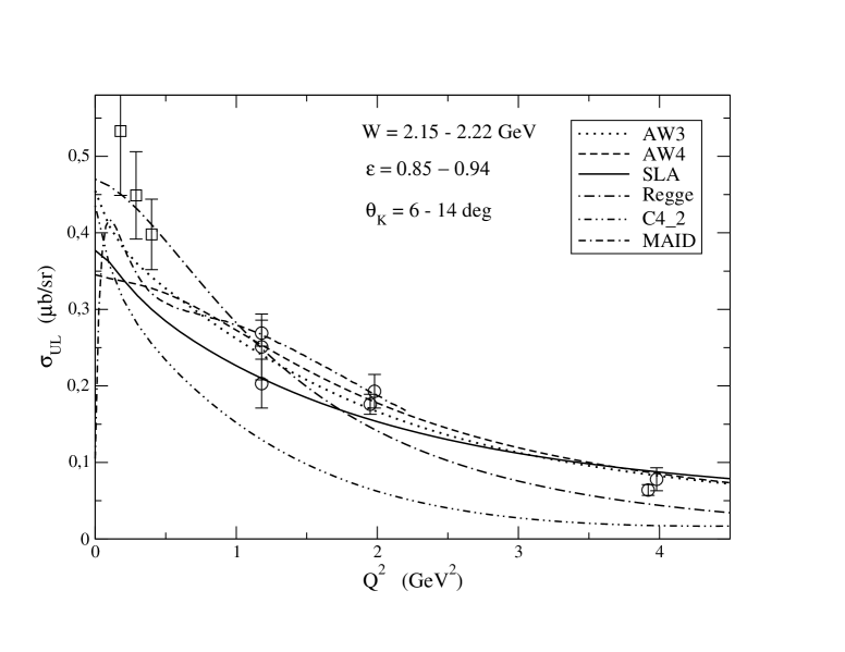
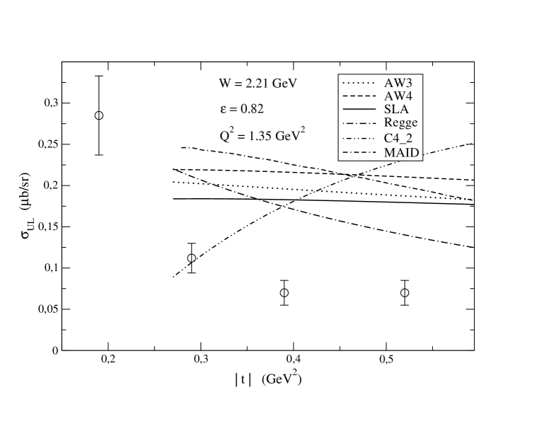
To reveal behaviour of the models in the kinematic region relevant for the E98-108 experiment, $W=1.8-2.2$ GeV and $Q^{2}=1.9-2.4$ GeV², in Figs. 4 and 5 we compare predictions of the models for the unpolarised cross section $\sigma_{UL}$ with old data by Bebek et al. [2], Brown et al. [32], and Brauel et al. [33]. In Figure 5 the data point at $|t|=0.19$ GeV² [33] is out of the physical region, for $W=2.21$ GeV starting at $|t|_{min}=0.26$ GeV², which is probably due to scaling the data from larger energies ($|t|_{min}=0.19$ GeV² for $W=2.43$ GeV). In Figure 4 calculations were performed at $W=2.18$ GeV, $\epsilon=0.91$, and $\theta_{K}^{cm}=11$ deg. Only the best predictions are shown in the both figures. The models AW3, AW4, SLA, MAID, and Regge can provide very good results for the $Q^{2}$-dependence, Fig. 4. Results of the models differ mainly at small $Q^{2}$ again where more precise data would be useful. Here the MAID model displays a pronounced bump structure similar to that for the separated cross sections (Fig. 3) but here it predicts very small, in comparison with the other models, photo-production cross section: $\sigma=105$ nb/sr (Fig. 4). The models fail in describing the t-dependence of $\sigma_{UL}$ the best results being achieved for $|t|_{min}$ (zero kaon angle), Fig. 5. The only Regge and MAID models provide a reasonable behaviour but they fail in normalisation of $\sigma_{UL}$. Predictions of the model C4 are out of the data in both Figures 4 and 5 (excluding at $|t|_{min}$ in Fig. 5). The model possesses a wrong t-dependence in addition and its results differ distinctly from predictions of the other models at forward kaon angles (Fig. 5).

3.2 Photo-production

In this subsection we discuss only the isobaric models because the energies assumed here are not high enough to be reasonable to apply the Regge model. The Regge model systematically over-predicts the photo-production data at photon energies less than 2 GeV as was shown in Fig. 3 and Ref. [30].

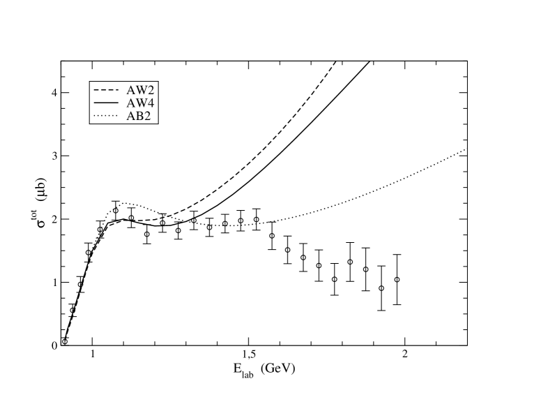
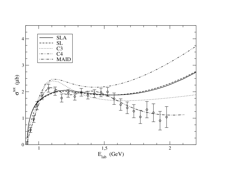
In Figures 6-8 we compare predictions of the models for the total cross section in the photo-production with SAPHIR data [25]. Relative errors of the data amount approximately to 8% excluding in the threshold region where it is around 15% and for energies higher than 1.5 GeV where it amounts up to 40% (see Figures 6-8). These data are therefore less restrictive than the unseparated electro-production cross sections for which the relative errors are less than 5%.

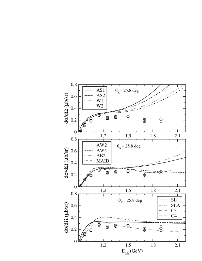
Predictions of the older models AS1, AS2, AW2, and AW4 are consistent with the data only up to $E_{\gamma}^{lab}=1.4$ GeV (Figs. 6 and 7) and those of W1, W2, AB2, and C4 up to $E_{\gamma}^{lab}=1.5$ GeV (Figs. 7 and 8). Apart from the C4 model the agreement with the data is within the expected range of validity of the models. The SL, SLA, and C3 models provide a satisfactory description of $\sigma^{tot}$ for the photon energy ranging up to 2 GeV (Fig. 8). Predictions of the SL and SLA models are very close each other. Better results are provided by the “off-shell extended” versions B and C of the Saclay-Lyon model (see Ref. [12] (Fig. 2)). The MAID model is in an excellent agreement with the data in the whole range of energies describing also their dip-bump structure (Fig. 8). This success is due to presence of the hadron form factors in the model as well as to the fit of the model parameters to the described data. The model attempted to explain the bump structure of the data around $E^{lab}_{\gamma}=1.5$ GeV by addition the “missing” resonance $D_{13}(1895)$ to the model. Inclusion of this resonance also improved behaviour of model predictions at higher energies [16].

Values of the $\chi^{2}$, calculated in analogy with Eq.(1) but for the total cross section and normalised to the number of the data points, are 2.47 and 5.17 for C3 and SLA models, respectively. Larger value for the SLA model is due to worse predictions of the model for $\sigma^{tot}$ near the threshold and for $E_{\gamma}^{lab}>1.6$ GeV than those of the C3 model. The model AB2 gives a very good agreement with data up to 1.6 GeV (Fig. 6), resulting in $\chi^{2}=5.10$ which is better than that for SLA. However, prediction of the AB2 is worse for $E_{\gamma}^{lab}>1.6$ GeV (Figs. 6 and 8) than that of SLA. The best value, $\chi^{2}=0.32$, was achieved by the MAID model whereas for C4 it amounts 11.6.

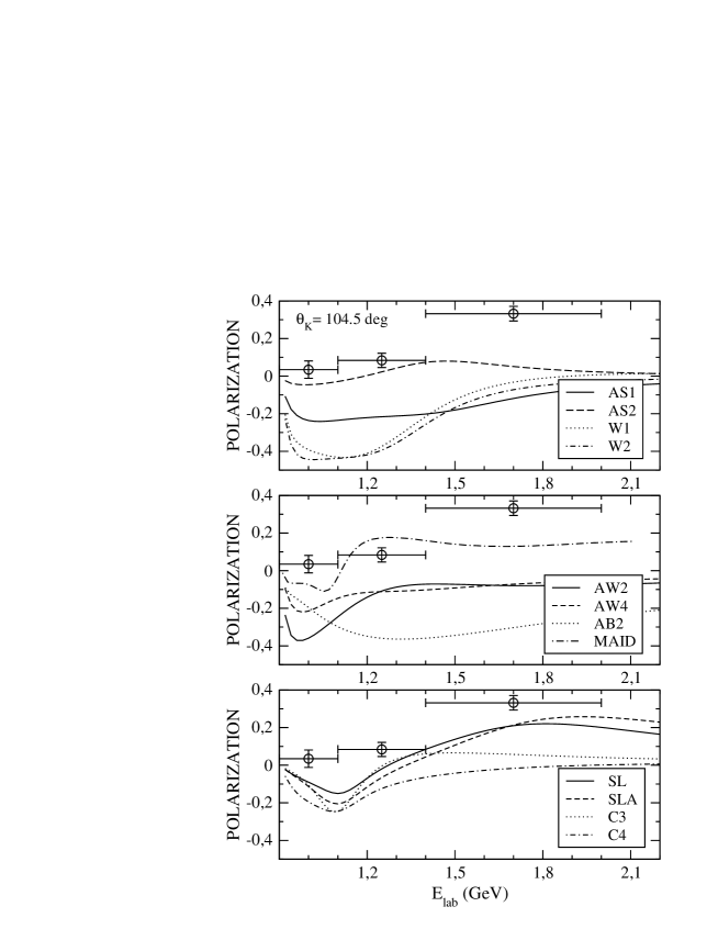
The SAPHIR data on the differential cross sections and polarizations [25] suffer from still larger error bars than those for $\sigma^{tot}$. Another disadvantage of the data is their averaging over bins of the photon energy and kaon angle. At this point one should also mention an apparent discrepancy of these SPHIR data with the older ones [34], especially at small kaon scattering angles [30]. However, we show a comparison of model predictions with the latest data here.

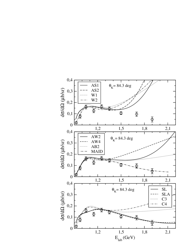
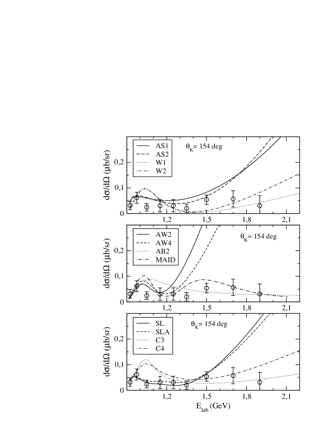
In Figs. 9-11 we display the differential cross section as a function of the photon lab energy for three values of the kaon c.m. angle. The older models AS1, AS2, W1, W2, AW2, AW4, and AB2 can describe the data satisfactorily only up to 1.4 GeV, even if the AB2, W1 and W2 models at 154 deg (Fig. 11) and the AW4 model at 25.8 deg (Fig. 9) can provide good results for energies up to 2 GeV. The models C3 and AW4 give very good results at small angles (Fig. 9) and high energies but they fail for larger angles and $E_{\gamma}^{lab}>1.4$ GeV (AW4) or $1<E_{\gamma}^{lab}<1.2$ GeV (C3) (Figs. 10 and 11). The model C4 systematically over-predicts the differential cross sections in most of the kinematic region discussed here, especially at forward angles which was already observed in Fig. 2. The SL and SLA models over-predict data at small angles especially near the threshold region. They provide very good description at intermediate angles but fail again at backward angles and $E_{\gamma}^{lab}>1.5$ GeV (Fig. 11) where results of the two models differ noticeably too. Evidently, the best result here is provided by the MAID model which can reproduce even the data structure. The model being regularised by the hadron form factors agree with the data for all angles even for $E_{\gamma}^{lab}=1.9$ GeV.

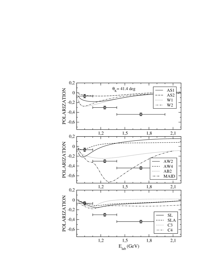
Situation with data accuracy is still worse for the lambda polarization asymmetry ($P$). That is why in Figs. 12 and 13 we show the energy bins over which data were averaged. At $\theta_{K}^{cm}=41.4$ deg (Fig. 12) the models except for MAID have a problem to describe the data points for $E_{\gamma}^{lab}>1.3$ GeV. The best result (in terms of $\chi^{2}$) was achieved by the MAID and AB2 models. At $\theta_{K}^{cm}=104.5$ deg (Fig. 13) the MAID, Saclay-Lyon, and AS2 (for $E_{\gamma}^{lab}<1.4$ GeV only) models give reasonable predictions. There is no need to say that more and better quality data are desirable here.

4 Conclusions

Among the tested models only the Saclay-Lyon A (SLA) and MAID can describe more or less all the discussed data. The Regge model is successful in predicting the electro-production cross sections but it cannot provide good results for the photo-production at energy less than 3-4 GeV. The Williams-Ji-Cotanch model C4 fails to describe the total cross section for the photo-production whereas C3 version cannot describe the new electro-production data. However, uncertainty in prescription for the electro-magnetic form factors does play a significant role for predictions of these models for the separated cross sections in the electro-production. The older models, Adelseck-Saghai (AS1, AS2), Workman (W1, W2), and Adelseck-Bennhold (AB2) are excluded by the new photo-production data, except for some cases where the models provide a reasonable results. These models, extended for the electro-production, cannot also predict the new data satisfactory. The analysis depends, however, to some extent on the prescription used for the electro-magnetic form factors. Large differences of the model predictions for the separated cross sections at small $Q^{2}$ call for other high accuracy electro-production data in that region.

In the kinematic region of the E98-108 experiment, $W=1.8-2.2$ GeV and $Q^{2}=1.9-2.4$ GeV², the SLA, Adelseck-Wright (AW4), Regge and MAID models are expected to provide reasonable results for the separated and unseparated cross sections whereas the unseparated cross sections merely can be predicted by the AW3 and C4 models in addition, where in the model C4 the electric ($G_{E}$) and magnetic ($G_{M}$) form factors are substituted in the electro-magnetic vertex [10].

5 Acknowledgements

Financial support from GA CR 202/02/0930 is gratefully acknowledged. Two of us (P.B. and M.S.) thank the INFN, Gruppo Sanità in Rome sincerely for its hospitality during completing this work.

Figure 1: Separated cross sections $\sigma_{T}$ and $\sigma_{L}$ and their ratio $R$ are shown as a function of $Q^{2}$ at $W=1.84$ GeV and zero kaon c.m. angle. Predictions of the models listed in Table 1 are plotted. The data are from Refs. [3] (circle), [4] (square), and [31] (solid square).

Figure 2: The same as in Fig.1 but for Williams-Ji-Cotanch models with different prescriptions for the electro-magnetic form factors (see sect. 2).

Figure 3: The same as in Fig.1 but for AW3, AW4, SLA, Regge, and MAID models.

Figure 4: Unseparated cross section for $\rm p(e,e^{\prime}K)\Lambda$ is shown as a function of $Q^{2}$. Calculations were performed at $W=2.18$ GeV, $\epsilon=0.91$, and $\theta_{K}^{cm}=11$ deg. The best predictions were shown only. The data are from Refs. [2] (circle) and [32] (square).

Figure 5: Unseparated cross section is shown as a function of the momentum transfer $|t|$. The physical region starts at $|t|_{min}=0.26$ GeV². The data are from Ref. [33].

Figure 6: Total cross sections for $\gamma\rm p\longrightarrow\Lambda K^{+}$ as predicted by AW2, AW4, and AB2 models are shown in dependence of the photon energy. The data are from Ref. [25].

Figure 7: The same as in Fig. 6 but for AS1, AS2, W1, and W2 models.

Figure 8: The same as in Fig.6 but for SLA, SL, C3, C4, and MAID models.

Figure 9: Differential cross section is shown as a function of the photon energy at kaon c.m. angle of 25.8 deg. The data are from Ref. [25].

Figure 10: The same as in Fig. 9 but for kaon angle of 84.3 deg.

Figure 11: The same as in Fig. 9 but for kaon angle of 154 deg.

Figure 12: Lambda polarization asymmetry is shown as a function of the photon energy at kaon c.m. angle of 41.4 deg. The data are from Ref. [25].

Figure 13: The same as in Fig. 12 but for kaon angle of 104.5 deg.

References

- [1] R.A. Adelseck and B. Saghai, Phys. Rev. C 42, 108 (1990).
- [2] C.J. Bebek, C.N. Brown, P. Bucksbaum, M. Herzlinger, S.D. Holmes, C.A. Lichtenstein, F.M. Pipkin, S.W. Raither, and L.K. Sisterson, Phys. Rev. D 15, 594 (1977).
- [3] G. Niculescu et al., Phys. Rev. Lett. 81, 1805 (1998).
- [4] R.M. Mohring et al., accepted to Phys. Rev. C; nucl-ex/0211005.
- [5] P. Markowitz, M. Iodice, S. Frullani, C.G. Chang, and O.K. Baker, “Electroproduction of Kaons up to Q2 = 3 (GeV/c)2”, Jefferson Lab Experimental proposal E98-108 approved for Hall A (1998); P. Markowitz, in Proc. 9th Int. Conf. On The Structure of Baryons, Newport News, Virginia, U.S.A., 3-8 Mar., 2002; M. Iodice, in Proc. Conf. Electron-Nucleus Scattering VII, Elba, Italy, 24-28 June, 2002, Eur. Phys. Jour. A (in press).
- [6] R.A. Adelseck, C. Bennhold, and L.E. Wright, Phys. Rev. C 32, 1681 (1985).
- [7] R.A. Adelseck and L.E. Wright, Phys. Rev. C 38, 1965 (1988).
- [8] R.L. Workman, Phys. Rev. C 44, 552 (1991).
- [9] R.A. Williams, Chueng-Ryong Ji, and S.R. Cotanch, Phys. Rev. C 43, 452 (1991).
- [10] R.A. Williams, Chueng-Ryong. Ji, and S.R. Cotanch, Phys. Rev. C 46, 1617 (1992).
- [11] J.C. David, C. Fayard, G.-H. Lamot, and B. Saghai, Phys. Rev. C 53, 2613 (1996).
- [12] T. Mizutani, C. Fayard, G.-H. Lamot, and B. Saghai, Phys. Rev. C 58, 75 (1998).
- [13] M. Guidal, J.-M. Laget, and M. Vanderhaeghen, Nucl. Phys. A 627, 645 (1997); Phys. Rev. C 61, 025204 (2000).
- [14] H. Thom, Phys. Rev. 151, 1322 (1966).
- [15] H. Haberzettl, C. Bennhold, T. Mart, and T. Feuster, Phys. Rev. C 58, R40 (1998); F.X. Lee, T. Mart, C. Bennhold, H. Haberzettl, L.E. Wright, Nucl. Phys. A 695, 237 (2001).
- [16] C. Bennhold, H. Haberzettl, and T. Mart, nucl-th/9909022; http://www.kph.uni-mainz.de/MAID/maid.html.
- [17] R.M. Davidson and R. Workman, Phys. Rev. C 63, 025210 (2001).
- [18] S. Janssen, J. Ryckebusch, D. Debruyne, and T. Van Cauteren, Phys. Rev. C 65, 015201 (2001).
- [19] T. Feuster and U. Mosel, Phys. Rev. C 58, 457 (1998).
- [20] Wen-Tai Chiang, F. Tabakin, T.-S.H. Lee, and B. Saghai, Phys. Lett. B 517, 101 (2001).
- [21] Zhenping Li, Phys. Rev. C 52, 1648 (1995).
- [22] D. Lu, R.H. Landau, and S.C. Phatak, Phys. Rev. C 52, 1662 (1995).
- [23] G.R. Farrar, K. Huleihel, and H. Zhang, Nucl. Phys. B 349, 655 (1991).
- [24] S. Steininger and U.-G. Meissner, Phys. Lett. B 391, 446 (1997).
- [25] M.Q. Tran et al. (SAPHIR Collaboration), Phys. Lett. B 445, 20 (1998).
- [26] M.F. Gari and W. Krümpelmann, Phys. Rev D 45, 1817 (1992).
- [27] M. Sotona and S. Frullani, Prog. Theor. Phys. 117, 151 (1994).
- [28] S. Capstick and W. Roberts, Rhys. Rev. D 49, 4570 (1994); ibid. 58, 074011 (1998).
- [29] B. Saghai, in Proc. Workshop on Hypernuclear Physics with Electromagnetic Probes, Hampton Uni., Virginia, U.S.A., 2-4 Dec., 1999, (eds. L. Tang and O. Hashimoto), p. 24.
- [30] P. Bydžovský, M. Sotona, O. Hashimoto, K. Itonaga, and T. Motoba, in Proc. Int. Workshop on ”Physics with GeV Electrons and Gamma-rays”, Sendai, Japan, 13-15 Feb., 2001, (eds. T. Tamae, J. Kasagi, T. Terasawa, and H. Yamazaki). Uni. Acad. Press, Inc., 2001, Tokyo, p.101.
- [31] A. Bleckmann, S. Herda, U. Opara, W. Schulz, W.J. Schwille, and H. Urbahn, Z. Phys. 239, 1 (1970).
- [32] C.N. Brown et al., Phys. Rev. Lett. 28, 1086 (1972).
- [33] P. Brauel, T. Canzler, D. Cords, R. Felst, G. Grindhammer, M. Helm,W.-D. Kollmann, H. Krehbiel, and M. Schädlich, Z. Phys. C 3, 101 (1979).
- [34] M. Bockhorst et al. (SAPHIR Collaboration), Z. Phys. C 63, 37 (1994).