Transverse momentum fluctuations due to temperature variation
in high-energy nuclear collisions

Abstract

The event-by-event $p_{\perp}-$fluctuations due to the temperature variations are considered. The so-called $\Phi-$measure is computed and shown to be a linear function of the temperature variance. The fluctuations of temperature naturally explain the data on $\Phi(p_{\perp})$ in proton-proton and central Pb-Pb collisions but independent measurements of the temperature fluctuations are needed to confirm the explanation. Feasibility of such an event-by-event measurement is discussed.

PACS: 25.75.-q, 25.75.Gz, 24.60.-k

Keywords: Relativistic heavy-ion collisions; Fluctuations; Thermal model

I Introduction

Predictions of different models of heavy-ion collisions are often quite similar when averaged characteristics of the collisions are considered. Fluctuations are usually much more sensitive to the collision dynamics and consequently can be helpful in discriminating among the models. Since large acceptance detectors, which have recently become common, make possible a detailed analysis of individual collisions the study of the event-by-event fluctuations appears to be a very promising field of high-energy heavy-ion physics, see [1] for a review.

The $p_{\perp}-$fluctuations in proton-proton and central Pb-Pb collisions at 158 GeV per nucleon have been recently measured [2] on event-by-event basis. To eliminate trivial ‘geometrical’ fluctuations due to the impact parameter variation, the so-called $\Phi-$measure [3] has been used. $\Phi$ is constructed is such a way that it is exactly the same for nucleon-nucleon (N-N) and nucleus-nucleus (A-A) collisions if the A-A collision is a simple superposition of the N-N interactions. In that case $\Phi$ is independent of the centrality of an A-A collision. Moreover, $\Phi$ equals zero when the inter-particle correlations are entirely absent. The critical analysis of the $\Phi-$measure can be found in [4, 5]. In the central Pb-Pb collisions the measured value of $\Phi(p_{\perp})$ equals $4.6\pm 1.5$ MeV while the preliminary result for proton-proton interactions in the same acceptance region is $5\pm 1$ MeV [2]. Although the two values are close, the mechanisms behind them seem to be different. It has been shown [2] that the correlations, which have short range in the momentum space, like those due to the quantum statistics, are responsible for the positive value of $\Phi(p_{\perp})$ in the central Pb-Pb collisions. When these correlations are subtracted $\Phi(p_{\perp})=0.6\pm 1.0$ MeV [2]. Our calculations have also demonstrated [6, 7] that the effect of Bose statistics of pions reduced by the hadron resonances fully explains the experimentally observed $\Phi(p_{\perp})=4.6\pm 1.5$ in the central Pb-Pb collisions. In the p-p case, the situation seems to be opposite - the short range correlations provide a negligible contribution to $\Phi(p_{\perp})$ while the whole effect is due to the long range fluctuations. Thus, the data suggest that the dynamical long range correlations are reduced in the central Pb-Pb collisions (when compared to p-p) with the short range caused by the Bose statistics being amplified. The former feature is a natural consequence of the system’s evolution towards the thermodynamic equilibrium. The amplification of the quantum statistics effect results from the increased particle population in the final state phase-space. Since various dynamical correlations contribute to $\Phi(p_{\perp})$ the question arises what is the dynamical correlation in the nucleon-nucleon interactions which appears to be absent in the central nucleus-nucleus collisions.

In the recent paper of the two of us [8], the correlation, which couples the average $p_{\perp}$ to the event multiplicity $N$, has been studied. The correlation is convincingly evidenced in the p-p collisions [9]. The approximate analytical formula of $\Phi(p_{\perp})$ as a function of the correlation strength has been derived and then the numerical simulation has been performed taking into account the finite detector’s acceptance. The effect of the correlation $\langle p_{\perp}\rangle$ vs. $N$ has been shown to be very weak if the particles from a small acceptance region are studied. Consequently, the correlation is far too small to explain the preliminary experimental value of $\Phi(p_{\perp})$ in the proton-proton collisions [2].

Our aim here is to discuss another possible mechanism responsible for the finite value of $\Phi(p_{\perp})$ in p-p interactions [2]. Namely, we analyze the effect of the temperature fluctuations. Its role in shaping the particle spectra has been studied before [10]. Here, the temperature, or more generally the slope parameter of the $p_{\perp}-$distribution, is assumed to vary from event to event. We compute $\Phi(p_{\perp})$ and find it to be a linear function of the temperature variance. As is well known [11], the $T-$variance is directly related to the system’s heat capacity. The idea to exploit the relationship to determine the specific heat of matter produced in nuclear collisions has been formulated in [12, 13], see also [14]. Since the temperature fluctuations have been shown [15] to yield the so-called non-extensive Tsallis statistics [16] (with a power-law instead of an exponential energy distribution) we express $\Phi(p_{\perp})$ by the non-extensivity parameter $q$. Further, we perform the numerical simulation of the p-p interactions with the effect of detector’s finite acceptance taken into account. The temperature fluctuations are shown to explain in a natural way the data on $\Phi(p_{\perp})$ in proton-proton and central Pb-Pb collisions. Finally, we discuss how to perform an independent measurement of the genuine temperature fluctuations which have to be extracted from the statistical noise.

II Analytical considerations

Let us first introduce the $\Phi-$measure. One defines a single-particle variable $z\buildrel\rm def\over{=}x-\overline{x}$ with the overline denoting average over a single particle inclusive distribution. Here, we identify $x$ with $p_{\perp}$ - the particle transverse momentum. The event variable $Z$, which is a multiparticle analog of $z$, is defined as $Z\buildrel\rm def\over{=}\sum_{i=1}^{N}(x_{i}-\overline{x})$, where the summation runs over particles from a given event. By construction, $\langle Z\rangle=0$, where $\langle...\rangle$ represents averaging over events. Finally, the $\Phi-$measure is defined in the following way

$$\Phi\buildrel\rm def\over{=}\sqrt{\langle Z^{2}\rangle\over\langle N\rangle}-\sqrt{\overline{z^{2}}}\;.$$ (1)

Various fluctuations or correlations contribute to (1). Our aim here is to compute $\Phi(p_{\perp})$ when the temperature varies from event to event. $P_{(T)}(p_{\perp})$ denotes the single particle transverse momentum distribution in events with temperature $T$ which is assumed to be independent of the event’s multiplicity $N$. As discussed in [10, 15], the temperature can vary within the event but we discard such a possibility and assume that there is single temperature characterizing every event. We will return to this point in the concluding section. Then, the inclusive transverse momentum distribution reads

$$P_{\rm incl}(p_{\perp})=\int_{0}^{\infty}dT\;{\cal P}(T)\;P_{(T)}(p_{\perp})\;,$$ (2)

where ${\cal P}(T)$ describes the temperature fluctuations. Consequently,

$$\overline{z^{2}}=\int_{0}^{\infty}dT\;{\cal P}(T)\int_{0}^{\infty}dp_{\perp}\;(p_{\perp}-\overline{p_{\perp}})^{2}P_{(T)}(p_{\perp})\;,$$ (3)

with

$$\overline{p_{\perp}}=\int_{0}^{\infty}dT\;{\cal P}(T)\int_{0}^{\infty}dp_{\perp}\;p_{\perp}\;P_{(T)}(p_{\perp})\;.$$

The $N-$particle transverse momentum distribution in the events of multiplicity $N$ is assumed to be the $N-$product of $P_{(T)}(p_{\perp})$ weighed by the multiplicity and temperature distributions. Therefore, all inter-particle correlations, different than those due to the temperature variations, are entirely neglected. Then, one finds

$$\langle Z^{2}\rangle=\sum_{N}{\cal P}_{N}\int_{0}^{\infty}dT\;{\cal P}(T)\int_{0}^{\infty}dp_{\perp}^{1}\;P_{(T)}(p_{\perp}^{1})\;.\;.\;.\int_{0}^{\infty}dp_{\perp}^{N}\;P_{(T)}(p_{\perp}^{N})\;\Big{(}p_{\perp}^{1}+.\;.\;.+p_{\perp}^{N}-N\overline{p_{\perp}}\Big{)}^{2}\;,$$ (4)

where ${\cal P}_{N}$ is the multiplicity distribution. Although the multi-particle distribution, Eq. (4), may look as a simple product of the one-particle distributions, the particle distributions are not independent from each other due to the integration over $T$.

In our further calculation we choose $P_{(T)}(p_{\perp})$ in the form suggested by the thermal model i.e.

$$P_{(T)}(p_{\perp})\sim p_{\perp}\exp\bigg{[}-{\sqrt{m^{2}+p_{\perp}^{2}}\over T}\bigg{]}\;,$$ (5)

where $m$ is the particle mass. If the transverse collective flow is taken into account $T$ should be understood as an effective temperature or simply a slope parameter controlled by the actual freeze-out temperature and the collective flow velocity.

In the limit $m=0$ the $p_{\perp}-$distribution (5) acquires a simple exponential form and one easily computes $\overline{z^{2}}$ and $\langle Z^{2}\rangle$ given by Eq. (3) and (4), respectively. Then, one gets

$$\overline{z^{2}} = 2\langle T^{2}\rangle+4(\langle T^{2}\rangle-\langle T\rangle^{2})$$

$${\langle Z^{2}\rangle\over\langle N\rangle} = 2\langle T^{2}\rangle+4{\langle N^{2}\rangle\over\langle N\rangle}\big{(}\langle T^{2}\rangle-\langle T\rangle^{2}\big{)}\;,$$

which gives

$$\Phi(p_{\perp})=\sqrt{2}\;{\langle N^{2}\rangle-\langle N\rangle\over\langle N\rangle}\;{\langle T^{2}\rangle-\langle T\rangle^{2}\over\langle T\rangle}\;,$$ (6)

when the $T-$fluctuations are sufficiently small i.e. $\langle N\rangle\langle T\rangle^{2}\gg\langle N^{2}\rangle(\langle T^{2}\rangle-\langle T\rangle^{2})$. For the poissonian multiplicity distribution the formula (6) simplifies to

$$\Phi(p_{\perp})=\sqrt{2}\;\langle N\rangle\;{\langle T^{2}\rangle-\langle T\rangle^{2}\over\langle T\rangle}\;.$$ (7)

III Interpretation of $\Phi$

If $T$ in Eq. (5) corresponds to genuine temperature, not a slope parameter, the formula (7) gets a nice interpretation due to the well-known thermodynamical relation [11] which has been discussed in the context of nuclear collisions in [12, 13, 14]. Namely,

$${1\over C_{v}}={\langle T^{2}\rangle-\langle T\rangle^{2}\over\langle T\rangle^{2}}\;,$$ (8)

where $C_{v}$ is the system’s heat capacity. We note that $C_{v}$, as an extensive thermodynamical parameter, is proportional to $\langle N_{\rm tot}\rangle$ which is the average number of all particles - charged and neutral - in the system at freeze-out, not to the average number of the observed particles $\langle N\rangle$ which enters Eq.  (7). Therefore, the formula (7) can be rewritten using the relation (8) as

$$\Phi(p_{\perp})=\sqrt{2}\;{\langle N\rangle\over\langle N_{\rm tot}\rangle}\;{\langle T\rangle\over c_{v}}\;,$$ (9)

with $c_{v}=C_{v}/\langle N_{\rm tot}\rangle$ being the specific heat of hadronic matter at freeze-out. For a system of massless non-interacting bosons with vanishing chemical potential $c_{v}=2\pi^{4}/15\zeta(3)\cong 10.8$. We note that $c_{v}$ is independent of the particle’s internal degrees of freedom.

A comment is in order here. It has been shown by one of us [6] that $\Phi(p_{\perp})$ vanishes in the ideal classical gas, where the particles are exactly independent from each other. On the other hand, the formula (9) tells us that $\Phi(p_{\perp})>0$ in such a gas. However, there is no conflict between the two results. The computation from [6] was performed at fixed temperature while the thermodynamical identity (8) states that there are temperature fluctuations in any system with finite heat capacity. In fact, these fluctuations are usually very small, because the temperature variance is inversely proportional to the number of particles. Consequently, the variations of temperature are neglected in most cases. However, $\Phi(p_{\perp})$ appears to be very sensitive to the temperature fluctuations and the two results differ qualitatively.

In the recent paper of one of us [15], the so-called non-extensive Tsallis statistics [16] has been shown to naturally emerge when a system experiences temperature fluctuations. Specifically, it has been argued [15] that $1/T$ often varies according to the gamma distribution. Then,

$${\cal P}(T)={\alpha^{\lambda}\over\Gamma(\lambda)}\Big{(}{1\over T}\Big{)}^{\lambda+1}{\rm exp}\Big{(}-{\alpha\over T}\Big{)}\;,$$ (10)

with the parameters $\lambda$ and $\alpha$ related to the moments of $1/T$ as

$$\Big{\langle}{1\over T}\Big{\rangle}={\lambda\over\alpha}\;,\;\;\;\;\;\;\;\;\Big{\langle}{1\over T^{2}}\Big{\rangle}-\Big{\langle}{1\over T}\Big{\rangle}^{2}={\lambda\over\alpha^{2}}\;.$$

Substituting Eqs. (5,10) into (2) one gets an inclusive distribution in the Tsallis statistics form [16]

$$P_{\rm incl}(p_{\perp})\sim p_{\perp}\Big{[}1+(q-1)\,{\sqrt{m^{2}+p_{\perp}^{2}}\over T_{0}}\;\Big{]}^{1\over 1-q}\;,$$ (11)

where $T_{0}\equiv\langle 1/T\rangle^{-1}$ and $q\equiv(\lambda+1)/\lambda$ is the non-extensivity parameter [16] related to the temperature fluctuations as [15]

$$q-1={\big{\langle}{1\over T^{2}}\big{\rangle}-\big{\langle}{1\over T}\big{\rangle}^{2}\over\big{\langle}{1\over T}\big{\rangle}^{2}}\cong{\langle T^{2}\rangle-\langle T\rangle^{2}\over\langle T\big{\rangle}^{2}}\;.$$ (12)

The second approximate equality holds for sufficiently small fluctuations. As known [16], the distribution (11) tends to (5) with $T=T_{0}$ when $q\rightarrow 1$. Using the relation (12), the formula (7) can be rewritten in yet another form,

$$\Phi(p_{\perp})=\sqrt{2}\;\langle N\rangle\;\langle T\rangle\;(q-1)\;,$$ (13)

which relates $\Phi$ to the non-extensivity parameter $q$.

The relationship between the $\Phi-$measure and Tsallis parameter $q$ has been earlier considered in a different context in [17]. Namely, the authors have studied how the $q-$statistics modifies the usual Bose-Einstein correlations discussed in [6, 7]. Then, $\Phi$ has been found to decrease, not increase as in Eq. (13), with $q$.

FIG. 1.: $\Phi(p_{T})$ as a function of the temperature variance for three values of the acceptance probability $p$. The temperature varies according to the gaussian distribution while the multiplicity is controlled by the lognormal one.

IV Numerical simulation

In this section we present the results of our Monte Carlo simulation of p-p collisions. The single-particle $p_{\perp}-$distribution is still given by Eq. (5). The mass equals now that of a charged pion because all particles in our simulation are treated as charged pions. We have considered two temperature distributions: the gamma-like form (10) and a gaussian distribution (cut off at $T<0$). The lognormal distribution of multiplicity of negative particles has been shown to fit the p-p data very well in the broad range of the collision energies [18]. We have used the parametrization given in [18] and assumed that the numbers of positive and negative pions are equal to each other in every event. The assumption is certainly reasonable in the central rapidity domain. To check whether the results are sensitive to the form of the multiplicity distribution we have also performed a simulation with the poissonian distribution of negative particles. As in the case of the lognormal distribution, the multiplicity of charged particles has been simply assumed to be two times bigger than that of negative ones. The average charged particle multiplicity and temperature have been taken as in our previous paper [8] i.e. $\langle T\rangle=167$ MeV and $\langle N\rangle=6.56$. These values correspond to the proton-proton collisions at 205 GeV.

FIG. 2.: $\Phi(p_{T})$ as a function of the temperature variance for three values of the acceptance probability $p$. The inverse temperature varies according to the gamma distribution while the multiplicity is controlled by the Poisson distribution.

Due to the particle registration inefficiency and finite detector’s coverage of the final state phase-space, only a fraction of the produced particles is usually observed in the experimental studies. Our Monte Carlo simulation takes into account the two effects in such a way that each generated particle - positive or negative pion - is registered with probability $p$ and rejected with $(1-p)$. The detector’s acceptance usually covers a given rapidity window but within our model the $T-$fluctuations and $p_{\perp}-$distribution are rapidity independent. Therefore, there is no difference between a particle being lost due to the limited acceptance and one lost due to the tracking inefficiency.

FIG. 3.: $\Phi(p_{T})$ as a function of the average number of observed particles for three values of the temperature variance. The temperature varies according to the gaussian distribution while the multiplicity is controlled by the lognormal one.

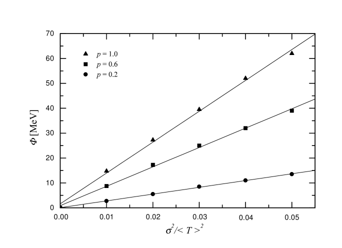
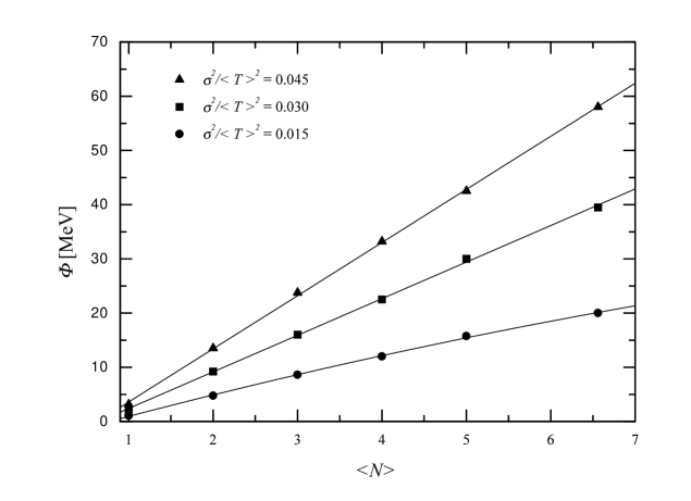
The results of our p-p simulation are shown in Figs. 1 - 4. Those in Figs. 1 and 3 have been found with the gaussian distribution of temperature and the lognormal multiplicity distribution. The results from Figs. 2 and 4 correspond to the gamma and Poisson distributions, respectively. When the gamma distribution is used the $T-$variance divided by $\langle T\rangle^{2}$ is denoted by $q-1$, in agreement with Eq. (12). In the case of gaussian distribution the same quantity is written as $\sigma^{2}/\langle T\rangle^{2}$. One sees in Figs. 1 and 2, that $\Phi(p_{T})$ grows linearly with the temperature variance, exactly as in Eq. (6). As can also be seen, the gaussian and gamma distributions yield very similar results. The two observations mean that the effect of finite pion mass is small and that $\Phi$, as in the $m=0$ case, is simply a linear function of the second moment of $T$.

FIG. 4.: $\Phi(p_{T})$ as a function of the average number of observed particles for three values of the temperature variance. The inverse temperature varies according to the gamma distribution while the multiplicity is controlled by the Poisson distribution.

Instead of the acceptance parameter $p$ one can use the average multiplicity of the observed particles $\langle N\rangle$ to characterize the acceptance. In Figs. 3 and 4 we present $\Phi(p_{T})$ as a function of $\langle N\rangle$. The growth of $\Phi(p_{T})$ with $\langle N\rangle$ is seen to be almost linear.

V Comparison with the experimental data

The preliminary experimental value of $\Phi(p_{T})$ in proton-proton collisions is, as already mentioned, $5\pm 1$ MeV [2]. The measurement has been performed in the transverse momentum and pion rapidity intervals (0.005, 1.5) GeV and (4.0, 5.5), respectively. Only about 20% of all produced particles have been observed. According to our simulation one needs $\sigma^{2}/\langle T\rangle^{2}=q-1\cong 0.015\pm 0.003$, which corresponds to $\sqrt{\langle T^{2}\rangle-\langle T\rangle^{2}}=20\pm 3$ MeV at $\langle T\rangle=167$ MeV, to reproduce the experimental result.

Let us now calculate the specific heat of the hadronic matter produced in the proton-proton interactions from the obtained value of $\sqrt{\langle T^{2}\rangle-\langle T\rangle^{2}}$. For that we identify $\langle N_{\rm tot}\rangle$ from Eq. (9) with the total number of pions. The pions include those ‘hidden’ in hadron resonances. We count each $\rho$ as two pions, each $\omega$ as three, etc. Then, $c_{v}$ from (9) is the heat capacity per pion. We estimate $\langle N_{\rm tot}\rangle$ as $5\cdot 1.5\cdot\langle N\rangle$, where the factor 5 is due to the acceptance and 1.5 to include the neutral particles. Then, one finds from Eq. (9) the heat capacity per pion $c_{v}=6\pm 2$. This number is significantly smaller than the previously mentioned specific heat of massless non-interacting bosons which equals 10.8. In fact, the discrepancy is even worse because a more realistic model of strongly interacting matter which takes into account numerous resonances and, obviously, finite hadron masses gives the heat capacity per pion exceeding 20 [14]. However, the very applicability of the thermodynamical model to the p-p collisions is far from obvious.

As discussed in the Introduction, $\Phi(p_{\perp})$, which is measured in the central Pb-Pb collisions, equals $4.6\pm 1.5$ MeV [2]. This value includes the short range (Bose-Einstein) correlations. When those correlations are excluded $\Phi(p_{\perp})=0.6\pm 1.0$ MeV [2]. Since the effect of quantum statistics is not taken into account in our simulation, this is the latter experimental value of $\Phi(p_{\perp})$ which should be compared with our calculation. The observed average multiplicity has been 270, i.e., as in the p-p interactions, about 20% of all produced charged particles [2]. We first identify the system freeze-out temperature with the slope parameter deduced from the pion transverse momentum distribution $\langle T\rangle\cong 180$ MeV [19]. Then, $\Phi(p_{\perp})=0.6\pm 1.0$ MeV yields via Eq. (7) $\sqrt{\langle T^{2}\rangle-\langle T\rangle^{2}}=0.5\pm 0.4$ MeV. Let us stress here that our numerical simulation fully confirms the reliability of the analytical formula (7). The temperature is significantly reduced if the transverse hydrodynamic expansion is taken into account. The freeze-out temperature obtained by means of the simultaneous analysis of the single particle spectra and the Bose-Einstein (HBT) correlations is about 120 MeV [19]. This temperature combined with $\Phi(p_{\perp})=0.6\pm 1.0$ MeV and $\langle N\rangle=270$ gives $\sqrt{\langle T^{2}\rangle-\langle T\rangle^{2}}=0.4\pm 0.4$ MeV. It has been argued in [14] that the transverse collective flow, which significantly modifies the observed temperature, does not contribute much to the slope parameter fluctuations. Therefore, the temperature variance is expected to be dominated by the genuine temperature fluctuations.

Calculating, as in the p-p case, the heat capacity per pion from the temperature dispersion, one finds that $\langle T\rangle=180$ MeV and $\sqrt{\langle T^{2}\rangle-\langle T\rangle^{2}}=0.5\pm 0.4$ MeV give $c_{v}=60\pm 100$ while $\langle T\rangle=120$ MeV and $\sqrt{\langle T^{2}\rangle-\langle T\rangle^{2}}=0.4\pm 0.4$ MeV correspond to $c_{v}=40\pm 70$. Unfortunately, the errors are so large that no conclusion can be drawn.

VI Measurement of $T-$fluctuations

In the previous section we have shown that the temperature fluctuations naturally explain the p-p and Pb-Pb data. Here, let us briefly consider how to observe independently the event-by-event temperature fluctuations. We discuss a straightforward method proposed in [20]. However, other procedures, in particular the so-called sub-event method developed in [21], might be more efficient. The temperature variance can be found measuring the event’s average transverse mass defined as

$$\mu_{\perp}={1\over N}\sum_{i=1}^{N}m^{i}_{\perp}\;,$$

where $N$ denotes the event’s multiplicity and $m_{\perp}^{i}=\sqrt{m^{2}+p_{\perp}^{i\,2}}$ is the transverse mass of $i-$th particle. If the single particle $p_{\perp}-$distribution is of the form (5) the $m_{\perp}-$distribution reads

$$P_{(T)}(m_{\perp})\sim m_{\perp}\>{\rm exp}\big{[}-{m_{\perp}\over T}\big{]}\;$$ (14)

and $\mu_{\perp}$ is related to $T$ in the following way

$$\mu_{\perp}=\int_{m}^{\infty}dm_{\perp}\>m_{\perp}\>P_{(T)}(m_{\perp})={2T^{2}+2Tm+m^{2}\over T+m}\;.$$

Then, the event’s temperature is expressed through $\mu_{\perp}$ as

$$T={1\over 4}\big{[}\sqrt{4m\mu_{\perp}-4m^{2}+\mu_{\perp}^{2}}+\mu_{\perp}-2m\big{]}\;.$$ (15)

Thus, measuring $\mu_{\perp}$ on the event-by-event basis one can get the temperature variance $V(T)=\langle T^{2}\rangle-\langle T\rangle^{2}$. However, the statistical fluctuations due to the finite event multiplicity have to be subtracted. The point is that when the genuine temperature does not fluctuate at all, the observed temperature does vary because the number of registered particles is not infinite.

When the genuine temperature is fixed and the particles are independent form each other the variance of $\mu_{\perp}$ is fully determined by the statistical fluctuations. In the events of multiplicity $N$ it equals

$$V_{s}(\mu_{\perp})={1\over N}\>V_{1}(m_{\perp})$$

where $V_{1}(m_{\perp})$ computed with the $m_{\perp}-$distribution (14) is

$$V_{1}(m_{\perp})={6T^{3}+6T^{2}m+3Tm^{2}+m^{3}\over T+m}-\Big{(}{2T^{2}+2Tm+m^{2}\over T+m}\Big{)}^{2}\;.$$ (16)

The $T-$variance is found from the $\mu_{\perp}-$variance in the usual way [22] i.e.

$$V_{s}(T)=\Big{(}{dT\over d\mu_{\perp}}\Big{)}^{2}V_{s}(\mu_{\perp})\;,$$ (17)

where the derivative is computed at $T=\langle T\rangle$ and $\mu_{\perp}=\langle\mu_{\perp}\rangle$. Since $T$ is not a linear function of $\mu_{\perp}$ Eq. (17) holds for sufficiently small $V_{s}(\mu_{\perp})$ [22]. This in turn demands that $N\gg 1$. Using Eq. (15), one finally finds the contribution of statistical fluctuations to the temperature variance as

$$V_{s}(T)={1\over 16}\bigg{[}{2m+\langle\mu_{\perp}\rangle\over\sqrt{4m\langle\mu_{\perp}\rangle-4m^{2}+\langle\mu_{\perp}\rangle^{2}}}+1\bigg{]}^{2}\;{V_{1}(m_{\perp})\over N}\;,$$ (18)

where $V_{1}(m_{\perp})$ is given by Eq. (16) with $T$ replaced by $\langle T\rangle$. We note that $V_{s}(T)=\langle T\rangle^{2}/N$ when $m=0$. The variance $V_{s}(T)$ should be subtracted from the observed $T-$variance $V(T)$ to eliminate the statistical fluctuations.

FIG. 5.: The observed $T-$variance as a function of multiplicity.

FIG. 6.: The $T-$variance with the subtracted statistical fluctuations as a function of the multiplicity.

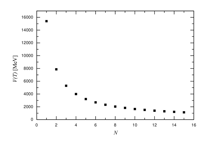
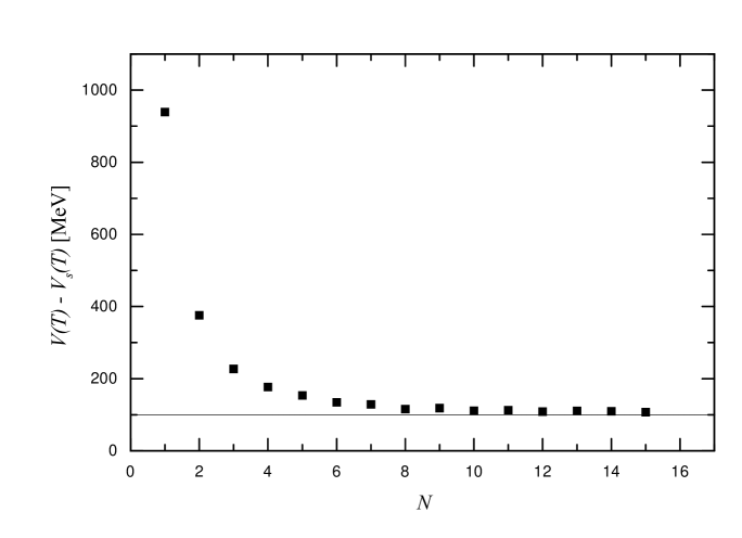
We have performed a simple simulation to see how well the subtraction procedure works. For this purpose we have generated the events with fixed multiplicity $N$ and temperature fluctuating from event to event. The single particle $p_{\perp}-$distribution has still been of the form (5) and the temperature varied according to the gaussian distribution with $\langle T\rangle=167$ MeV. The event temperature has been determined in the ‘experimental’ way described above. Finally, the temperature variance has been found and the statistical contribution has been subtracted. In Figs. 5 and 6 we show $V(T)$ and $V(T)-V_{s}(T)$ as a function of the event multiplicity. One can see that in spite of large values of $V(T)$ and $V_{s}(T)$ the input temperature variance $\sigma^{2}=100\;{\rm MeV}^{2}$ is well reproduced for $N$ as small as 10. The result, although expected, is not entirely trivial. The expression (18) assumes that the particles are independent from each other while in our simulation the particles are correlated because of the temperature fluctuations. We conclude that the measurement of $T-$fluctuations seems to be a feasible task even in the case of relatively low multiplicity collisions.

VII Final remarks

We have shown that $\Phi(p_{\perp})$ observed in proton-proton collisions [2] can be understood as an effect of temperature fluctuations with $\sqrt{\langle T^{2}\rangle-\langle T\rangle^{2}}=20$ MeV. While the result needs to be confirmed by independent $T-$variance measurements let us mention here an interesting observation from [23]. It has been found there that the transverse mass spectrum of $\pi^{0}$ from p-p collisions at $\sqrt{s}=30$ GeV decreases as $p_{\perp}^{-P}$ over 10 orders of magnitude with $P=9.6$. Within the thermal model, such a behavior naturally appears due to the temperature fluctuations [15]. Then, the exponent $P=9.6$ gives the non-extensivity parameter in Eq. (11) equal $q=1.10$ which translates into $\sqrt{\langle T^{2}\rangle-\langle T\rangle^{2}}=53$ MeV at $\langle T\rangle=167$ MeV. The two values of the temperature dispersion extracted from the p-p data, 20 MeV and 53 MeV, have been found in different ways. One easily shows that $\Phi$ is mostly sensitive to the event-by-event temperature fluctuations while the inclusive distribution is shaped both by the temperature variation from event to event and within the event. Therefore, the $T-$dispersion found from the inclusive spectrum is expected to be larger than that from $\Phi$.

$\Phi(p_{\perp})$ observed in the central Pb-Pb collisions is very small when the short range correlations are subtracted [2]. This small value corresponds to the temperature dispersion below 1 MeV. The difference of the dispersions found in p-p and central Pb-Pb collisions is not surprising. The hadronic system from nuclear interactions is not only larger - $\Phi$ as an intensive quantity is not directly dependent on the system size - but at freeze-out it is expected to be much closer to the thermodynamic equilibrium. Consequently, the temperature fluctuations should be smaller.

We conclude our considerations as follows. The event-by-event fluctuations of temperature are a possible mechanism determining the value of $\Phi(p_{\perp})$ in p-p collisions. The smallness of the contribution of the long range correlations to $\Phi(p_{\perp})$ in the central Pb-Pb collisions is then also naturally explained. One needs an independent measurement of the temperature variance to confirm the explanation. Since the sizable fluctuations due to the finite statistics are, in principle, under control, such a measurement seems to be feasible even in the relatively low multiplicity interactions.